
MFTransNet: A Multi-Modal Fusion with CNN-Transformer Network for Semantic Segmentation of HSR Remote Sensing Images

Abstract
:1. Introduction
- A multi-modal semantic segmentation model MFTransNet, which combines CNN and Transformer, is proposed, and achieves a balance of accuracy and speed.
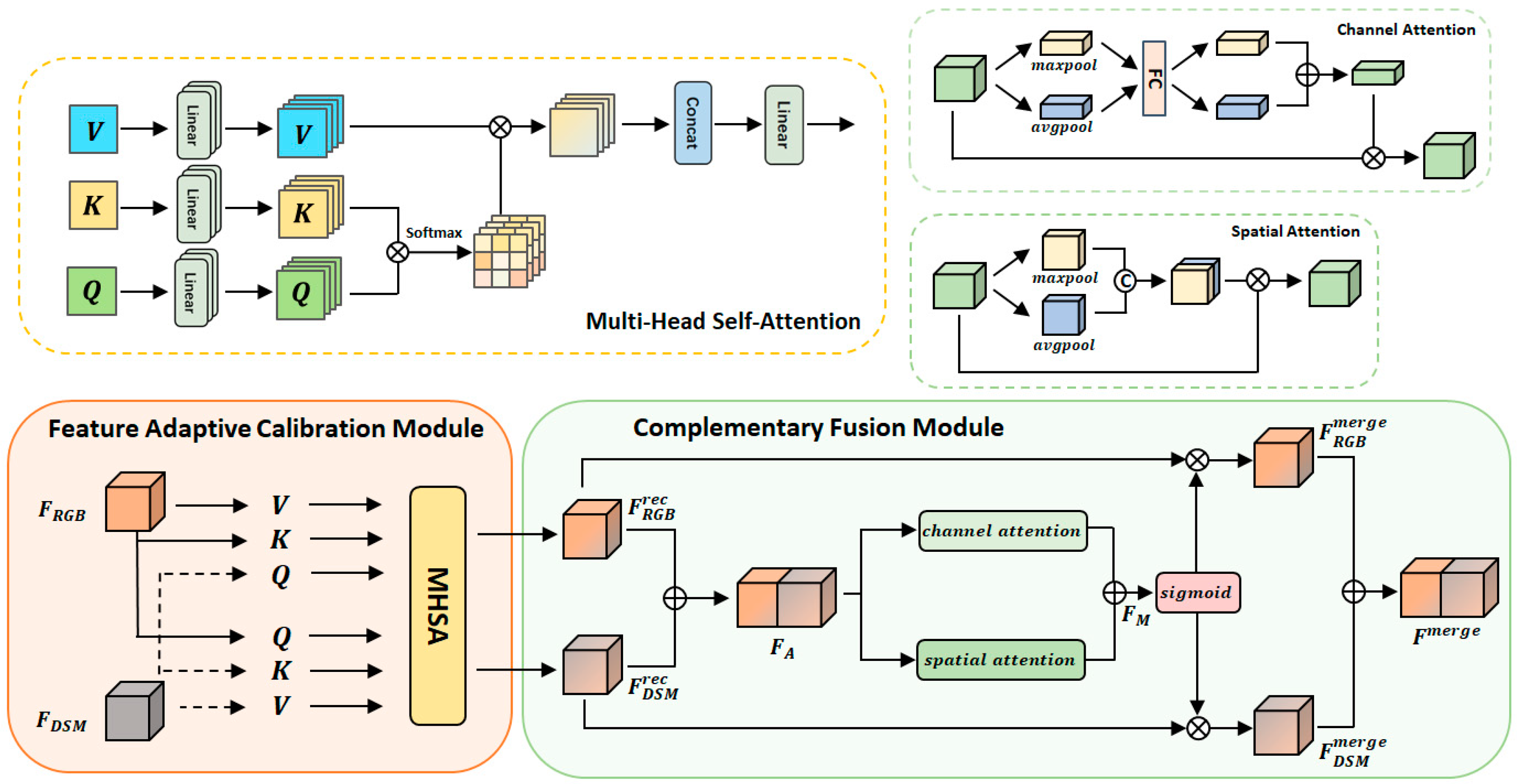
- A feature fusion module containing a multi-head attention mechanism, a feature adaptive calibration module (FACM) for adaptively calibrating features, and a complementary fusion module (CFM) for fusing multi-modal features, are proposed to achieve the efficient adaptive fusion of features.
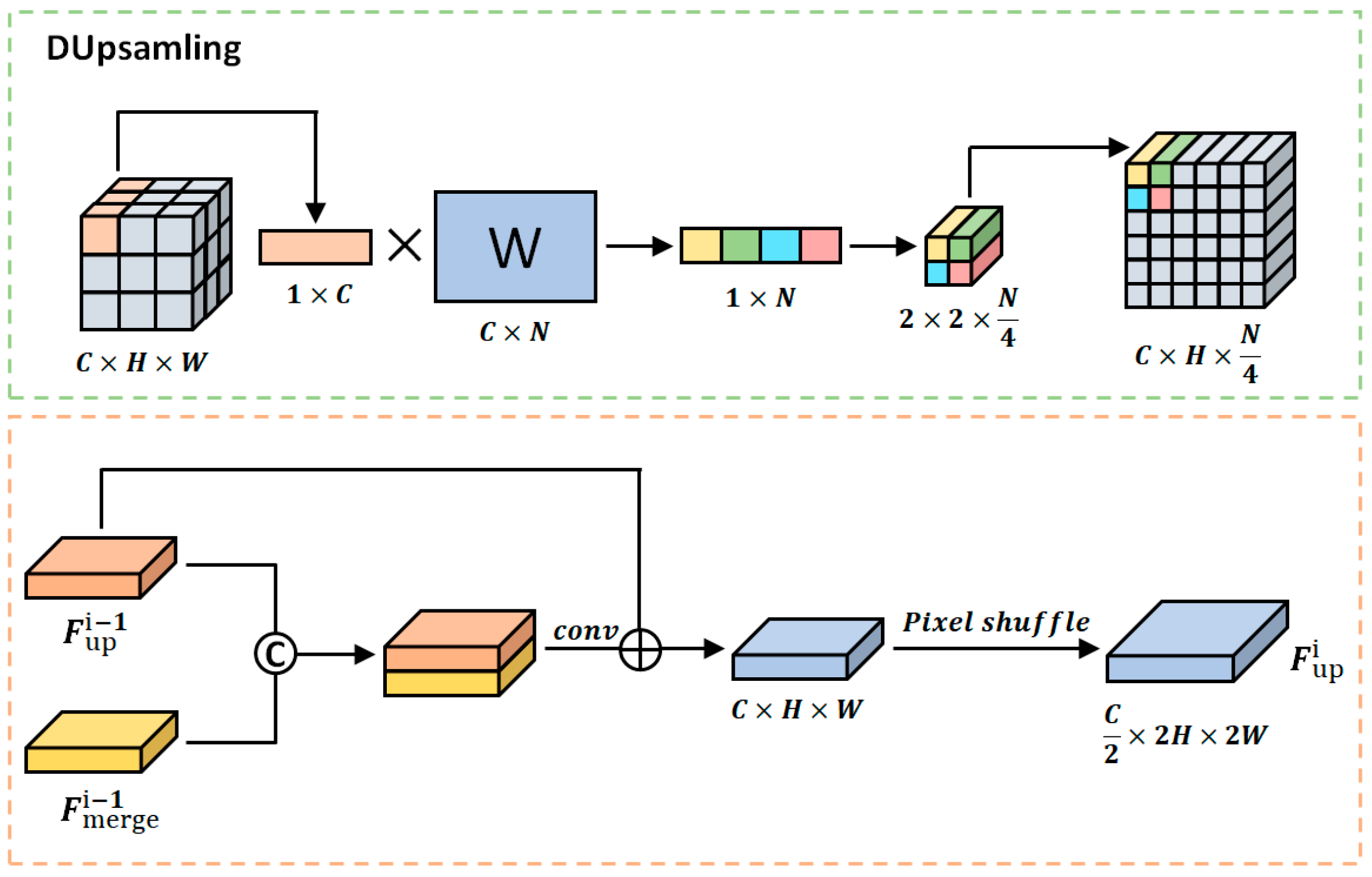
- A multi-scale decoder is used for the multi-scale problem in remote sensing images, and DUpsampling [16] is used instead of the traditional bilinear upsampling to reduce the details lost in the upsampling process and to achieve feature aggregation at different scales.
- While ensuring task completion, a model with a lower number of parameters and more streamlined structure is obtained through channel compression and an optimized structure. Meanwhile, we skillfully use channel shuffle and PixelShuffle on feature extraction and decoder. The optimized model requires fewer computational resources and can meet a wider range of application requirements than the original model. The proposed model achieves a SOTA effect on the Potsdam dataset.
2. Related Work
2.1. Semantic Segmentation of Remote Sensing Images
2.2. Transformer
2.3. Multi-Modal Data Fusion
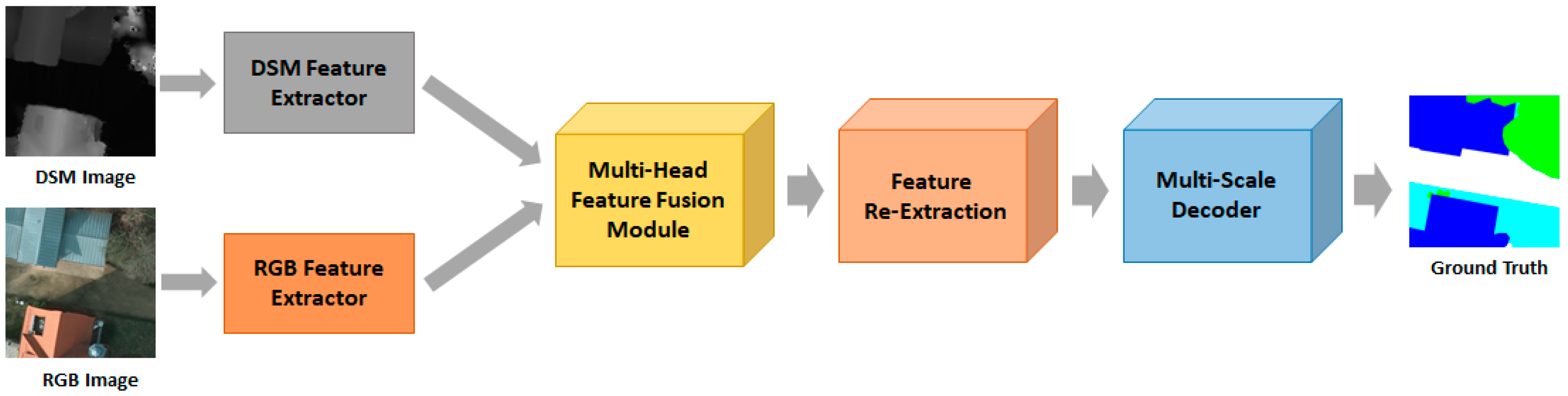
3. Proposed Method
3.1. Backbone Network
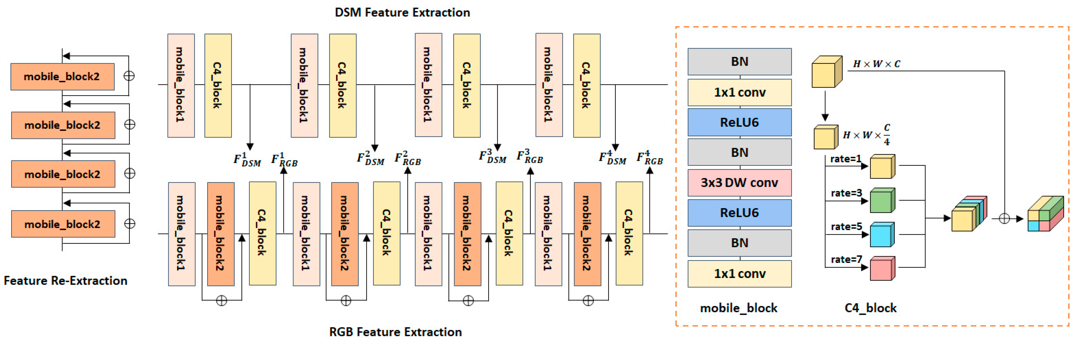
3.2. Feature Extraction Module
3.3. Multi-Head Feature Fusion Module
3.4. Multi-Scale Decoder
4. Experiment
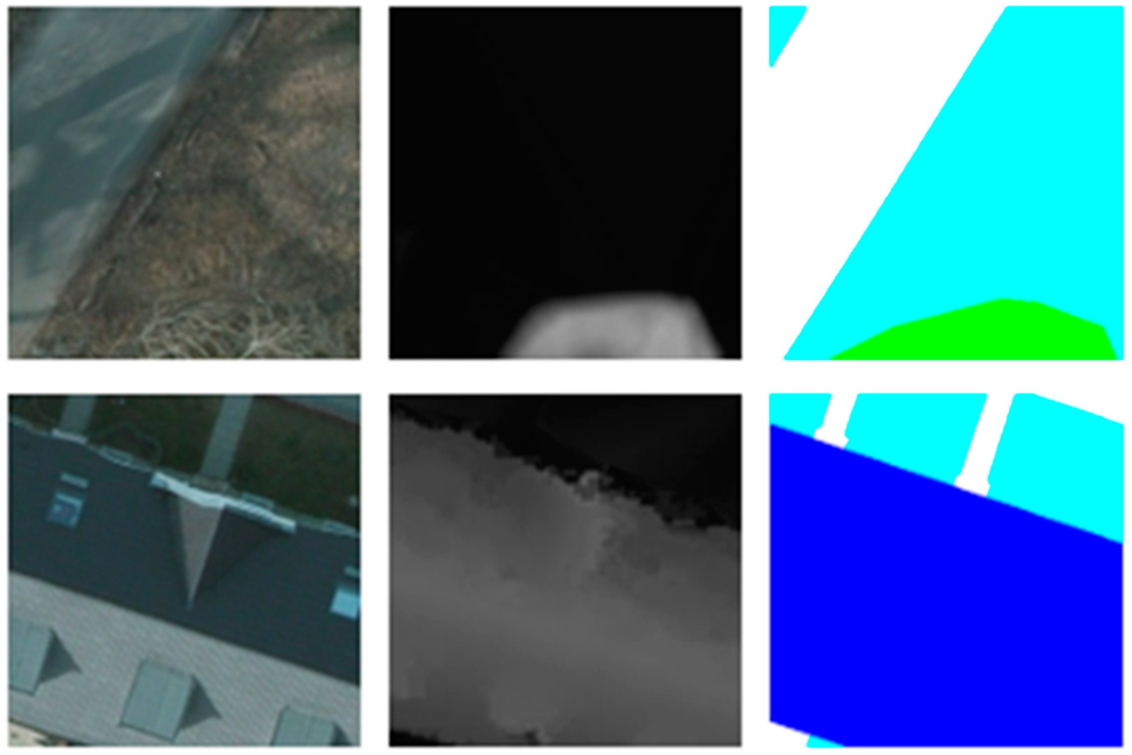
4.1. Dataset
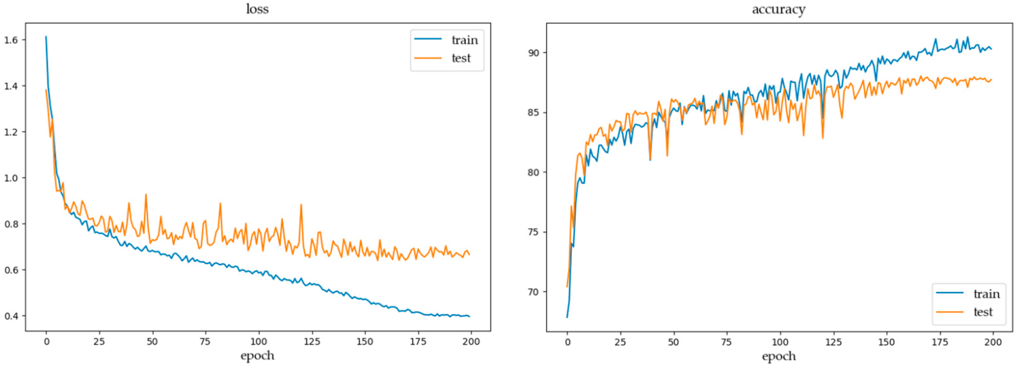
4.2. Implementation Details
4.3. Evaluation
4.4. Experiment
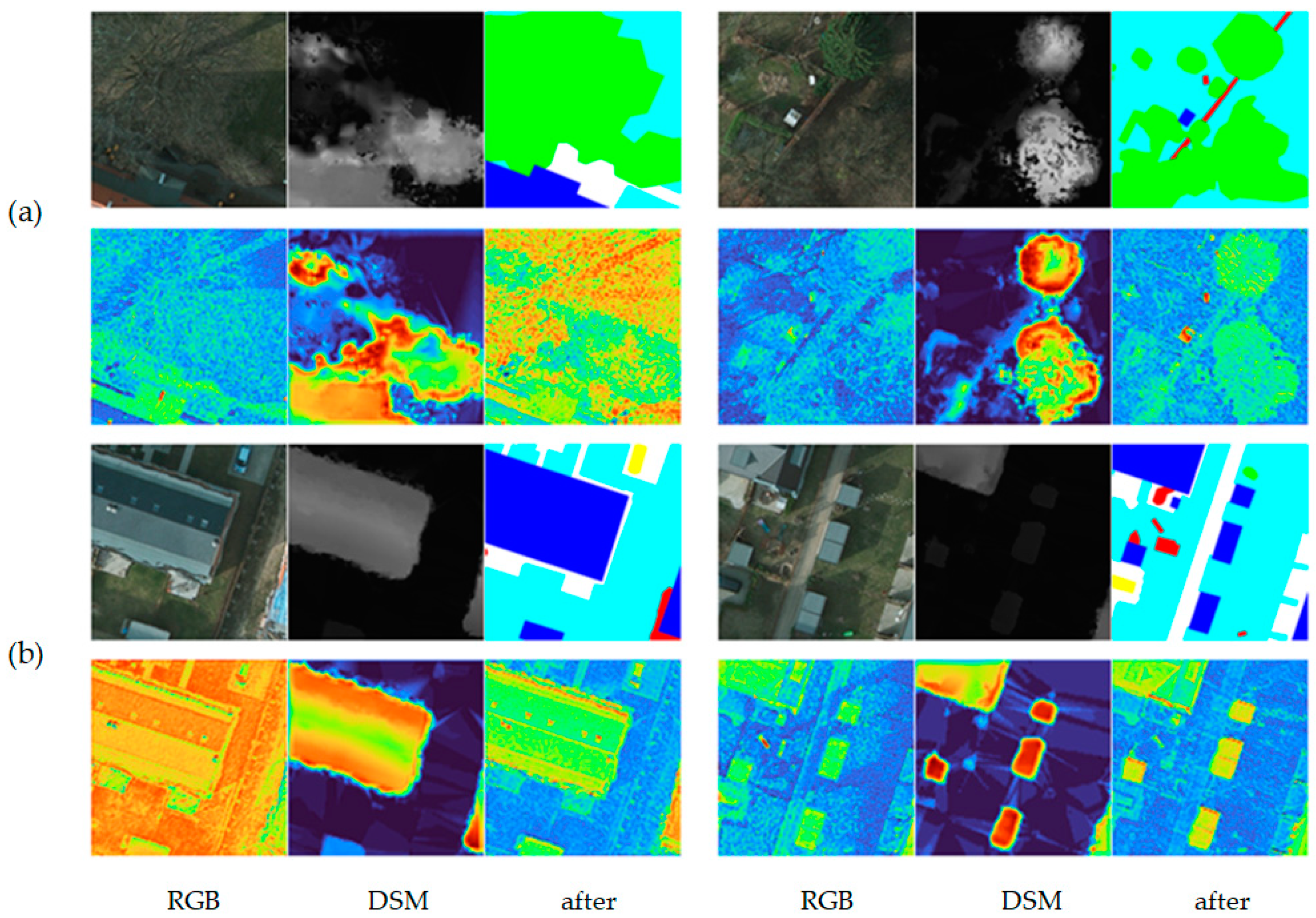
4.5. Feature Visualization
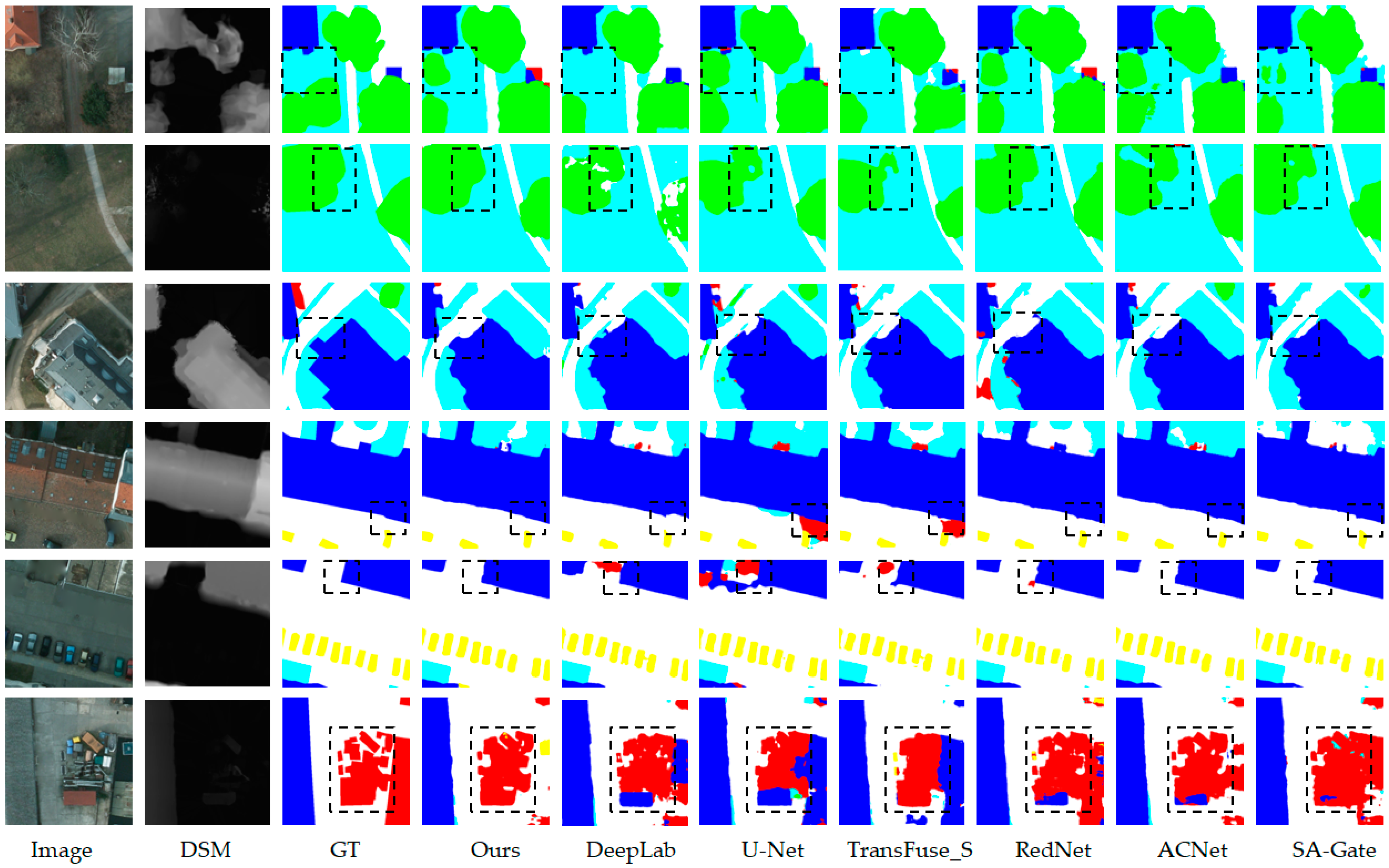
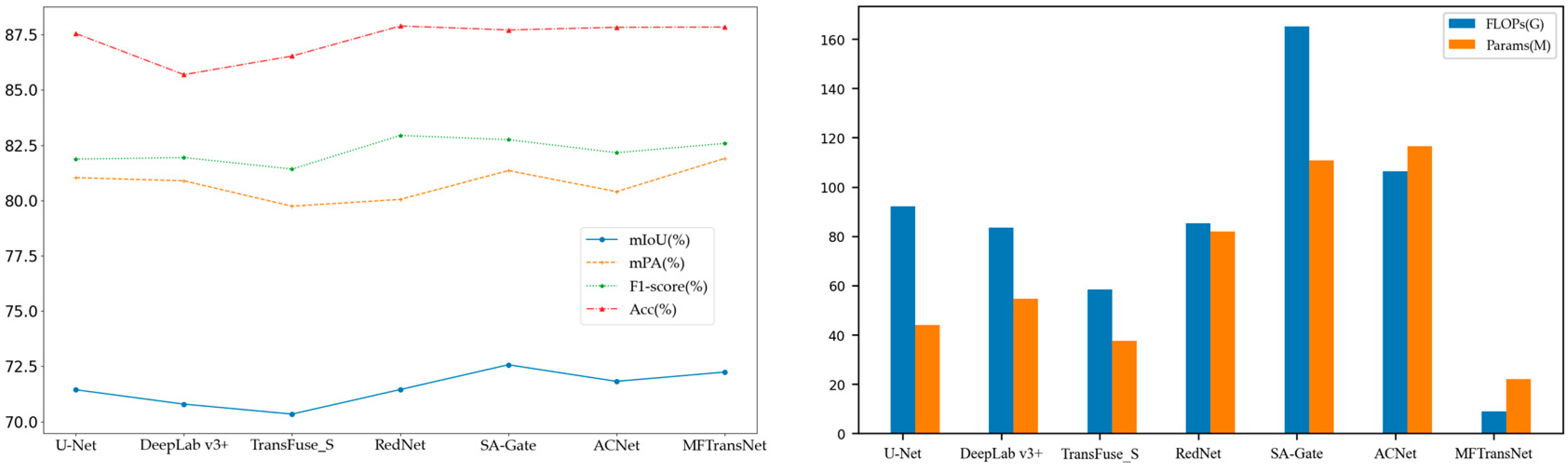
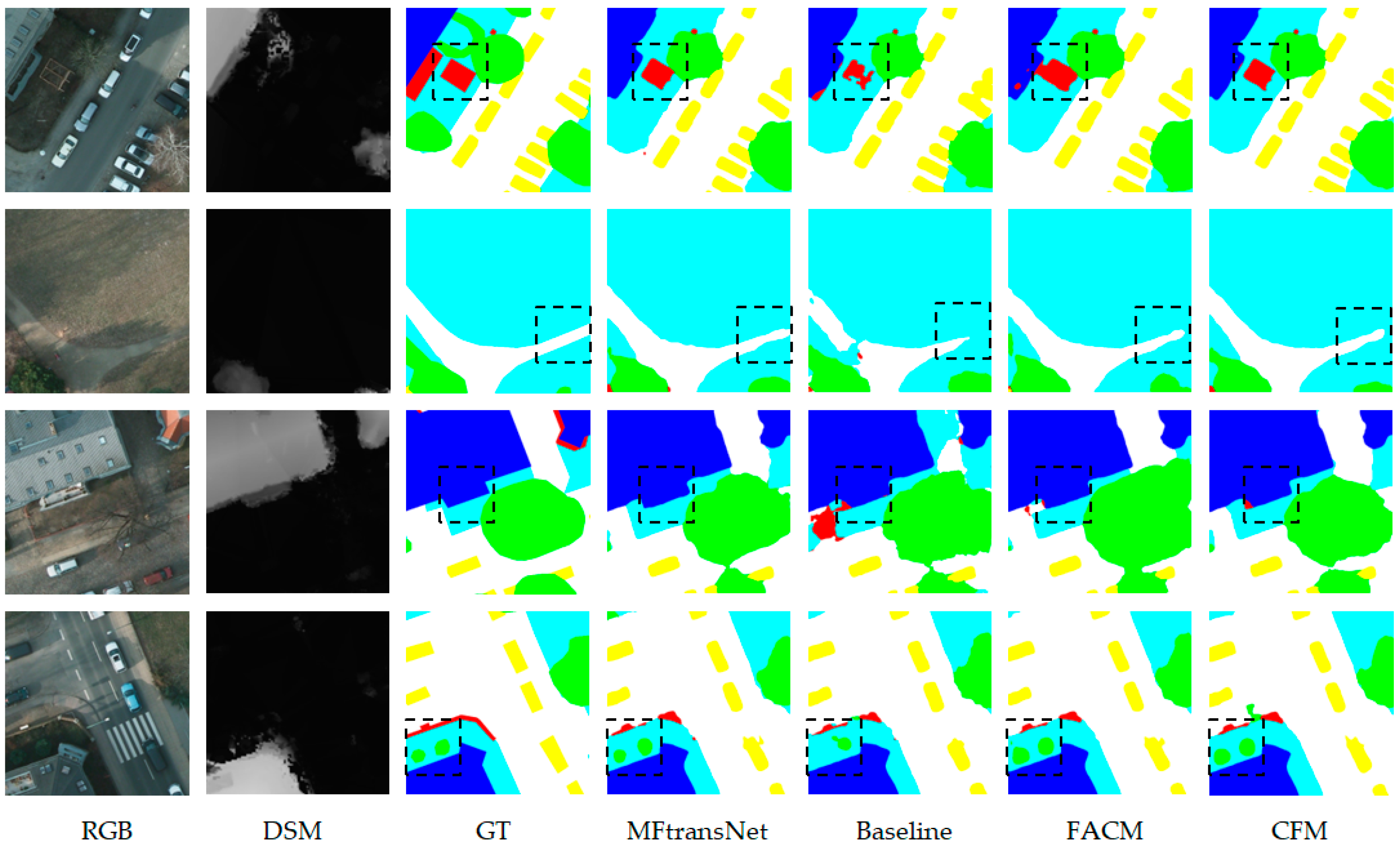
4.6. Comparative Experiments
4.7. Ablation Experiments
5. Conclusions
Author Contributions
Funding
Data Availability Statement
Conflicts of Interest
References
- Ha, Q.; Watanabe, K.; Karasawa, T.; Ushiku, Y.; Harada, T. MFNet: Towards real-time semantic segmentation for autonomous vehicles with multi-spectral scenes. In Proceedings of the 2017 IEEE/RSJ International Conference on Intelligent Robots and Systems (IROS), Vancouver, BC, Canada, 24–28 September 2017. [Google Scholar]
- Chen, H.; Shi, Z. A Spatial-Temporal Attention-Based Method and a New Dataset for Remote Sensing Image Change Detection. Remote Sens. 2020, 12, 1662. [Google Scholar] [CrossRef]
- Chen, K.; Fu, K.; Yan, M.; Gao, X.; Sun, X.; Wei, X. Semantic Segmentation of Aerial Images with Shuffling Convolutional Neural Networks. IEEE Geosci. Remote Sens. Lett. 2018, 15, 173–177. [Google Scholar] [CrossRef]
- Zheng, X.; Wang, B.; Du, X.; Lu, X. Mutual Attention Inception Network for Remote Sensing Visual Question Answering. IEEE Trans. Geosci. Remote Sens. 2021, 60, 1–14. [Google Scholar] [CrossRef]
- Zheng, X.; Gong, T.; Li, X.; Lu, X. Generalized Scene Classification from Small-Scale Datasets with Multitask Learning. IEEE Trans. Geosci. Remote Sens. 2022, 60, 1–11. [Google Scholar] [CrossRef]
- Le, N.Q.K. Potential of deep representative learning features to interpret the sequence information in proteomics. Proteomics 2022, 22, e2100232. [Google Scholar] [CrossRef]
- Kha, Q.-H.; Ho, Q.-T.; Le, N.Q.K. Identifying SNARE Proteins Using an Alignment-Free Method Based on Multiscan Convolutional Neural Network and PSSM Profiles. J. Chem. Inf. Model. 2022, 62, 4820–4826. [Google Scholar] [CrossRef] [PubMed]
- Albulayhi, K.; Smadi, A.A.; Sheldon, F.T.; Abercrombie, R.K. IoT Intrusion Detection Taxonomy, Reference Architecture, and Analyses. Sensors 2021, 21, 6432. [Google Scholar] [CrossRef]
- Abu Al-Haija, Q.; Krichen, M. A Lightweight In-Vehicle Alcohol Detection Using Smart Sensing and Supervised Learning. Computers 2022, 11, 121. [Google Scholar] [CrossRef]
- Alsulami, A.A.; Abu Al-Haija, Q.; Alqahtani, A.; Alsini, R. Symmetrical Simulation Scheme for Anomaly Detection in Autonomous Vehicles Based on LSTM Model. Symmetry 2022, 14, 1450. [Google Scholar] [CrossRef]
- Kareem, S.S.; Mostafa, R.R.; Hashim, F.A.; El-Bakry, H.M. An Effective Feature Selection Model Using Hybrid Metaheuristic Algorithms for IoT Intrusion Detection. Sensors 2022, 22, 1396. [Google Scholar] [CrossRef]
- Cao, Z.; Fu, K.; Lu, X.; Diao, W.; Sun, H.; Yan, M.; Yu, H.; Sun, X. End-to-End DSM Fusion Networks for Semantic Segmenta-tion in High-Resolution Aerial Images. IEEE Geosci. Remote Sens. Lett. 2019, 16, 1766–1770. [Google Scholar] [CrossRef]
- Sun, Y.; Cao, B.; Zhu, P.; Hu, Q. Drone-based RGB-Infrared Cross-Modality Vehicle Detection via Uncertainty-Aware Learning. IEEE Trans. Circuits Syst. Video Technol. 2020, 32, 6700–6713. [Google Scholar] [CrossRef]
- Lang, F.; Yang, J.; Yan, S.; Qin, F. Superpixel Segmentation of Polarimetric Synthetic Aperture Radar (SAR) Images Based on Generalized Mean Shift. Remote Sens. 2018, 10, 1592. [Google Scholar] [CrossRef]
- Xie, E.; Wang, W.; Yu, Z.; Anandkumar, A.; Álvarez, J.M.; Luo, P. SegFormer: Simple and Efficient Design for Semantic Segmentation with Transformers. Neural Inf. Process Syst. 2021, 34, 12077–12090. [Google Scholar]
- Tian, Z.; He, T.; Shen, C.; Yan, Y. Decoders Matter for Semantic Segmentation: Data-Dependent Decoding Enables Flexible Feature Aggregation. In Proceedings of the 2019 IEEE/CVF Conference on Computer Vision and Pattern Recognition (CVPR), Long Beach, CA, USA, 15–20 June 2019; pp. 3121–3130. [Google Scholar]
- Shelhamer, E.; Long, J.; Darrell, T. Fully convolutional networks for semantic segmentation. IEEE Trans. Pattern Anal. Mach. Intell. 2017, 39, 640–651. [Google Scholar] [CrossRef]
- Chen, L.-C.; Zhu, Y.; Papandreou, G.; Schroff, F.; Adam, H. Encoder-Decoder with Atrous Separable Convolution for Semantic Image Segmentation; Springer International Publishing: Cham, Switzerland, 2018; pp. 833–851. [Google Scholar]
- Chen, L.C.; Papandreou, G.; Kokkinos, I.; Murphy, K.; Yuille, A.L. Semantic Image Segmentation with Deep Convolutional Nets and Fully Connected CRFs. arXiv 2014, arXiv:1412.7062. [Google Scholar]
- Chen, L.C.; Papandreou, G.; Kokkinos, I.; Murphy, K.; Yuille, A.L. DeepLab: Semantic Image Segmentation with Deep Convolutional Nets, Atrous Convolution, and Fully Connected CRFs. IEEE Trans. Pattern Anal. Mach. Intell. 2017, 40, 834–848. [Google Scholar] [CrossRef]
- Chen, L.C.; Papandreou, G.; Schroff, F.; Adam, H. Rethinking Atrous Convolution for Semantic Image Seg-mentation. arXiv 2017, arXiv:1706.05587. [Google Scholar]
- Ronneberger, O.; Fischer, P.; Brox, T. U-Net: Convolutional Networks for Biomedical Image Segmentation. In Medical Image Computing and Computer-Assisted Intervention—MICCAI 2015; Springer International Publishing: Cham, Switzerland, 2015; pp. 234–241. [Google Scholar]
- Badrinarayanan, V.; Kendall, A.; Cipolla, R. Segnet: A deep convolutional encoder-decoder architecture for image segmentation. IEEE Trans. Pattern Anal. Mach. Intell. 2017, 39, 2481–2495. [Google Scholar] [CrossRef]
- Noh, H.; Hong, S.; Han, B. Learning Deconvolution Network for Semantic Segmentation. In Proceedings of the 2015 IEEE International Conference on Computer Vision (ICCV), Santiago, Chile, 7–13 December 2015; pp. 1520–1528. [Google Scholar]
- Zheng, Z.; Zhong, Y.; Wang, J.; Ma, A. Foreground-Aware Relation Network for Geospatial Object Segmentation in High Spatial Resolution Remote Sensing Imagery. In Proceedings of the 2020 IEEE/CVF Conference on Computer Vision and Pattern Recognition (CVPR), Seattle, WA, USA, 13–19 June 2020; pp. 4095–4104. [Google Scholar]
- Du, X.; He, S.; Yang, H.; Wang, C. Multi-Field Context Fusion Network for Semantic Segmentation of High-Spatial-Resolution Remote Sensing Images. Remote Sens. 2022, 14, 5830. [Google Scholar] [CrossRef]
- Niu, R.; Sun, X.; Tian, Y.; Diao, W.; Chen, K.; Fu, K. Hybrid Multiple Attention Network for Semantic Segmentation in Aerial Images. IEEE Trans. Geosci. Remote Sens. 2021, 60, 1–18. [Google Scholar] [CrossRef]
- Ma, A.; Wang, J.; Zhong, Y.; Zheng, Z. FactSeg: Foreground Activation-Driven Small Object Semantic Segmentation in Large-Scale Remote Sensing Imagery. IEEE Trans. Geosci. Remote Sens. 2021, 60, 1–16. [Google Scholar] [CrossRef]
- Wang, L.; Li, R.; Duan, C.; Zhang, C.; Meng, X.; Fang, S. A Novel Transformer Based Semantic Segmentation Scheme for Fine-Resolution Remote Sensing Images. IEEE Geosci. Remote Sens. Lett. 2022, 19, 1–5. [Google Scholar] [CrossRef]
- Vaswani, A.; Shazeer, N.; Parmar, N.; Uszkoreit, J.; Jones, L.; Gomez, A.N.; Kaiser, L.; Polosukhin, I. Attention is all you need. In Proceedings of the 31st Conference on Neural Information Processing Systems (NIPS 2017), Long Beach, CA, USA, 4–9 December 2017; pp. 5998–6008. [Google Scholar]
- Dosovitskiy, A.; Beyer, L.; Kolesnikov, A.; Weissenborn, D.; Zhai, X.; Unterthiner, T.; Dehghani, M.; Minderer, M.; Heigold, G.; Gelly, S.; et al. An image is worth 6x16 words: Transformers for image recognition at scale. arXiv 2021, arXiv:2010.11929. [Google Scholar]
- Zheng, S.; Lu, J.; Zhao, H.; Zhu, X.; Luo, Z.; Wang, Y.; Fu, Y.; Feng, J.; Xiang, T.; Torr, P.H.; et al. Rethinking Semantic Segmentation from a Sequence-to-Sequence Perspective with Transformers. In Proceedings of the IEEE/CVF Conference on Computer Vision and Pattern Recognition, Nashville, TN, USA, 20–25 June 2021; pp. 6877–6886. [Google Scholar] [CrossRef]
- Srinivas, A.; Lin, T.-Y.; Parmar, N.; Shlens, J.; Abbeel, P.; Vaswani, A. Bottleneck Transformers for Visual Recogni-tion. arXiv 2021, arXiv:2101.11605. [Google Scholar]
- Guo, J.; Han, K.; Wu, H.; Tang, Y.; Chen, X.; Wang, Y.; Xu, C. CMT: Convolutional Neural Networks Meet Vision Transformers. In Proceedings of the IEEE/CVF Conference on Computer Vision and Pattern Recognition, New Orleans, LA, USA, 18–24 June 2022; pp. 12165–12175. [Google Scholar] [CrossRef]
- Gulati, A.; Qin, J.; Chiu, C.C.; Parmar, N.; Zhang, Y.; Yu, J.; Han, W.; Wang, S.; Zhang, Z.; Wu, Y.; et al. Conformer: Convolution-augmented Transformer for Speech Recognition. In Proceedings of the Interspeech 2020, Shanghai, China, 25–29 October 2020. [Google Scholar]
- Chen, J.; Lu, Y.; Yu, Q.; Luo, X.; Adeli, E.; Wang, Y.; Lu, L.; Yuille, A.L.; Zhou, Y. TransUNet: Transformers Make Strong Encoders for Medical Image Segmentation. arXiv 2021, arXiv:2102.04306. [Google Scholar]
- Chen, X. Bi-directional Cross-Modality Feature Propagation with Separation-and-Aggregation Gate for RGB-D Semantic Segmentation. arXiv 2020, arXiv:2007.09183. [Google Scholar]
- Liu, H.; Chen, F.; Zeng, Z.; Tan, X. AMFuse: Add–Multiply-Based Cross-Modal Fusion Network for Multi-Spectral Semantic Segmentation. Remote Sens. 2022, 14, 3368. [Google Scholar] [CrossRef]
- Weng, Q.; Chen, H.; Chen, H.; Guo, W.; Mao, Z. A Multisensor Data Fusion Model for Semantic Segmentation in Aerial Images. IEEE Ge-Oscience Remote Sens. Lett. 2022, 19, 1–5. [Google Scholar] [CrossRef]
- Prakash, A.; Chitta, K.; Geiger, A. Multi-Modal Fusion Transformer for End-to-End Autonomous Driving. In Proceedings of the IEEE/CVF Conference on Computer Vision and Pattern Recognition, Nashville, TN, USA, 20–25 June 2021. [Google Scholar]
- Cao, Z.; Diao, W.; Sun, X.; Lyu, X.; Yan, M.; Fu, K. C3Net: Cross-Modal Feature Recalibrated, Cross-Scale Semantic Aggregated and Compact Network for Semantic Segmentation of Multi-Modal High-Resolution Aerial Images. Remote Sens. 2021, 13, 528. [Google Scholar] [CrossRef]
- Zhao, J.; Zhang, D.; Shi, B.; Zhou, Y.; Chen, J.; Yao, R.; Xue, Y. Multi-source collaborative enhanced for remote sensing images semantic segmentation. Neurocomputing 2022, 493, 76–90. [Google Scholar] [CrossRef]
- Liu, H.; Zhang, J.; Yang, K.; Hu, X.; Stiefelhagen, R. CMX: Cross-Modal Fusion for RGB-X Semantic Segmentation with Transformers. arXiv 2022, arXiv:2203.04838. [Google Scholar]
- Wele, G.; Patel, V.M. HyperTransformer: A Textural and Spectral Feature Fusion Transformer for Pansharpening. arXiv 2022, arXiv:2203.02503. [Google Scholar]
- Sandler, M.; Howard, A.; Zhu, M.; Zhmoginov, A.; Chen, L. MobileNetV2: Inverted residuals and linear bottlenecks. In Proceedings of the IEEE/CVF Conference on Computer Vision and Pattern Recognition (CVPR), Salt Lake City, UT, USA, 18–23 June 2018; pp. 4510–4520. [Google Scholar] [CrossRef]
- Zhang, Y.; Liu, H.; Hu, Q. TransFuse: Fusing Transformers and CNNs for Medical Image Segmentation. In Proceedings of the Medical Image Computing and Computer Assisted Intervention–MICCAI 2021: 24th International Conference, Strasbourg, France, 27 September–1 October 2021; pp. 14–24. [Google Scholar] [CrossRef]
- Hu, X.; Yang, K.; Fei, L.; Wang, K. ACNET: Attention based network to exploit complementary features for rgbd semantic segmentation. In Proceedings of the IEEE Conference on Image Processing (ICIP), Taipei, Taiwan, 22–25 September 2019; pp. 1440–1444. [Google Scholar]
- Jiang, J.; Zheng, L.; Luo, F.; Zhang, Z. RedNet: Residual encoderdecoder network for indoor RGB-D semantic segmentation. arXiv 2018, arXiv:1806.01054. [Google Scholar]


| Method | Years | Approach | Advantages | Disadvantages |
|---|---|---|---|---|
| FCN | 2014 | Use convolutional layers instead of fully connected layers | An input image of any size can be accepted | A lot of storage overhead; Coarse segmentation effect |
| Deeplab V3+ | 2018 | Dilated convolution and bilinear upsampling are used | Multi-scale feature extraction is achieved | The segmentation effect of high-resolution image is poor |
| U-Net | 2015 | The encoder-decoder structure and skip connection are used | Support for a small number of trained models | Redundancy leads to slow training |
| SegNet | 2017 | Confirm the position after upsampling using pooling indices | Low memory requirements | The accuracy improvement is not high |
| DeconvNet | 2015 | Add the deconvolution layer on top of vgg | It is stronger than FCN in segmentation details | Boundary segmentation is not accurate |
| FarSeg | 2020 | Explicit foreground modeling approach | Mitigating foreground and background imbalances | - |
| MCFNet | 2022 | Confidence-based local selection criterion | Optimal balance between segmentation accuracy, storage efficiency and inference speed | - |
| HMANet | 2020 | A collection of three category-based attention modules | Improve discrimination between classes | - |
| FactSeg | 2022 | It consists of a two-branch decoder and a joint probabilistic loss | Small object features are activated and large-scale background noise is suppressed | - |
| DC-Swin | 2022 | Designed a densely connected feature aggregation module decoder | Enhanced semantic space and channel relations features | - |
| ViT | 2021 | The image patches are directly input into the Transformer for feature extraction | The effect is better than SOTA’s CNN when trained with a large amount of data | A large amount of data is required for training |
| Setr | 2021 | Introducing Transformer from the perspective of semantic segmentation | The receptive field of the model is improved | Large number of parameters and computations |
| BotNet | 2021 | Replace the bottleneck in the fourth block in ResNet with the Multi-Head Self-Attention Module | Both efficiency and accuracy are improved | - |
| CMT | 2021 | The key and value computation is replaced by the deep convolution computation in the main module | The computational cost is reduced | - |
| Conformer | 2020 | It consists of a CNN branch and a Transformer branch | Enhanced global perception of local features and local details of global representations | High model complexity |
| TransUnet | 2021 | Resnet and ViT are combined using the U-Net structure | Higher performance than various methods in medical applications | High model complexity |
| SA-Gate | 2020 | Propose a unified, efficient cross-modal guidance coder | Information from different models is effectively integrated | - |
| MCENet | 2022 | Designed a co-enhanced fusion module | It is more competitive in terms of the number of parameters and inference speed | - |
| AMFuse | 2022 | Efficiently combine multiplication and addition operations | Effectiveness in fusing RGB and thermal information | - |
| MSDFM | 2022 | Color digital surface model data is used as additional input | The segmentation accuracy of small objects is improved | The segmentation accuracy is not high for low vegetation and trees |
| TransFuser | 2021 | Using attention to integrate image and LiDAR representation | Achieving state-of-the-art performance in complex driving scenarios | - |
| C3Net | 2021 | Using a cross-modal feature recombination module | A balance between accuracy and speed is achieved | - |
| CMX | 2022 | Two backbones are used to extract RGB and other modes, respectively | The generalization performance of outdoor scenes is excellent | Large number of parameters |
| Attributes | Categories | |||||
|---|---|---|---|---|---|---|
| Name | Impervious Surface | Building | Low Vegetation | Tree | Car | Clutter |
| Color |  |  |  |  |  |  |
| Train set | 29.95% | 24.56% | 23.43% | 15.53% | 1.55% | 4.98% |
| Test set | 34.29% | 25.39% | 18.84% | 14.99% | 2.04% | 4.45% |
| Method | Impervious Surface | Building | Low Vegetation | Tree | Car | Clutter | mIoU | mPA | ||||||
|---|---|---|---|---|---|---|---|---|---|---|---|---|---|---|
| IoU | PA | IoU | PA | IoU | PA | IoU | PA | IoU | PA | IoU | PA | |||
| U-Net | 81.78 | 88.32 | 89.47 | 95.14 | 69.28 | 86.4 | 72.89 | 83.6 | 82.34 | 87.89 | 32.85 | 44.8 | 71.44 | 81.03 |
| DeepLab v3+ | 78.43 | 91.72 | 87.33 | 91.24 | 65.99 | 80.51 | 71.2 | 77.66 | 81.73 | 89.15 | 40.06 | 55.02 | 70.79 | 80.89 |
| TransFuse_S | 80.86 | 91.09 | 88.4 | 93.42 | 68.74 | 85.71 | 70.58 | 78.93 | 81.47 | 89.58 | 32.01 | 39.69 | 70.34 | 79.74 |
| ACNet | 83.44 | 91.15 | 92.73 | 97.26 | 69.05 | 83.57 | 71.57 | 85.13 | 81.84 | 87.6 | 30.08 | 35.6 | 71.45 | 80.05 |
| RedNet | 82.83 | 92.45 | 92.4 | 96.09 | 69.64 | 83.68 | 71.5 | 81.47 | 83.06 | 89.89 | 35.96 | 44.52 | 72.57 | 81.35 |
| SA-Gate | 82.74 | 91.82 | 91.33 | 96.42 | 70.52 | 86.87 | 69.88 | 77.9 | 79.56 | 85.31 | 36.88 | 44.08 | 71.82 | 80.4 |
| MFTransNet | 83.26 | 91.09 | 91.92 | 95.54 | 70.28 | 86.44 | 72.26 | 82.37 | 82.08 | 90.83 | 33.87 | 43.96 | 72.34 | 81.7 |
| Method | Backbone | FLOPs (G) | Params (M) | F1-Score (%) | Acc (%) |
|---|---|---|---|---|---|
| U-Net | Resnet50 | 92.12 | 43.93 | 81.87 | 87.55 |
| DeepLab v3+ | Xception | 83.44 | 54.71 | 81.94 | 85.69 |
| TransFuse_S | Resnet34 | 58.36 | 37.61 | 81.42 | 86.53 |
| RedNet | Resnet50 | 85.26 | 81.95 | 82.94 | 87.89 |
| SA-Gate | Resnet101 | 165.1 | 110.85 | 82.75 | 87.71 |
| ACNet | Resnet50 | 106.25 | 116.60 | 82.16 | 87.83 |
| MFTransNet | - | 9.91 | 23.20 | 82.57 | 87.93 |
| Method | FACM | CFM | mIoU | mPA | F1-Score (%) | Acc (%) |
|---|---|---|---|---|---|---|
| Baseline | 70.91 | 81.07 | 81.99 | 86.99 | ||
| Ours | √ | 71.57 | 80.77 | 81.84 | 87.64 | |
| Ours | √ | 71.59 | 80.5 | 82.9 | 87.68 | |
| Ours | √ | √ | 72.34 | 81.7 | 82.57 | 87.93 |
| Method | Impervious Surface | Building | Low Vegetation | Tree | Car | Clutter | ||||||
|---|---|---|---|---|---|---|---|---|---|---|---|---|
| IoU | PA | IoU | PA | IoU | PA | IoU | PA | IoU | PA | IoU | PA | |
| Baseline | 81.34 | 88.09 | 91.38 | 97.2 | 68.13 | 85.91 | 70.13 | 81.09 | 79.57 | 91.47 | 34.94 | 42.64 |
| With FACM | 82.34 | 91.41 | 91.7 | 95.27 | 70.64 | 83.89 | 72.64 | 84.62 | 81.24 | 88.86 | 30.88 | 40.57 |
| With CFM | 82.52 | 91.26 | 91.56 | 95.83 | 69.98 | 86.0 | 71.65 | 81.83 | 80.12 | 87.73 | 33.74 | 40.33 |
| MFTransNet | 83.26 | 91.09 | 91.92 | 95.54 | 70.28 | 86.44 | 72.26 | 82.37 | 82.08 | 90.83 | 33.87 | 43.96 |
Disclaimer/Publisher’s Note: The statements, opinions and data contained in all publications are solely those of the individual author(s) and contributor(s) and not of MDPI and/or the editor(s). MDPI and/or the editor(s) disclaim responsibility for any injury to people or property resulting from any ideas, methods, instructions or products referred to in the content. |
© 2023 by the authors. Licensee MDPI, Basel, Switzerland. This article is an open access article distributed under the terms and conditions of the Creative Commons Attribution (CC BY) license (https://creativecommons.org/licenses/by/4.0/).
Share and Cite
He, S.; Yang, H.; Zhang, X.; Li, X. MFTransNet: A Multi-Modal Fusion with CNN-Transformer Network for Semantic Segmentation of HSR Remote Sensing Images. Mathematics 2023, 11, 722. https://doi.org/10.3390/math11030722
He S, Yang H, Zhang X, Li X. MFTransNet: A Multi-Modal Fusion with CNN-Transformer Network for Semantic Segmentation of HSR Remote Sensing Images. Mathematics. 2023; 11(3):722. https://doi.org/10.3390/math11030722
Chicago/Turabian StyleHe, Shumeng, Houqun Yang, Xiaoying Zhang, and Xuanyu Li. 2023. "MFTransNet: A Multi-Modal Fusion with CNN-Transformer Network for Semantic Segmentation of HSR Remote Sensing Images" Mathematics 11, no. 3: 722. https://doi.org/10.3390/math11030722