Article

PCEP: Few-Shot Model-Based Source Camera Identification

School of Information and Communication Engineering, Dalian University of Technology, Dalian 116024, China
*
Author to whom correspondence should be addressed.
Mathematics 2023, 11(4), 803; https://doi.org/10.3390/math11040803
Submission received: 1 January 2023 / Revised: 31 January 2023 / Accepted: 1 February 2023 / Published: 4 February 2023
(This article belongs to the Special Issue Mathematical Methods for Computer Science)

Abstract

:
Source camera identification is an important branch in the field of digital forensics. Most existing works are based on the assumption that the number of training samples is sufficient. However, in practice, it is unrealistic to obtain a large amount of labeled samples. Therefore, in order to solve the problem of low accuracy for existing methods in a few-shot scenario, we propose a novel identification method called prototype construction with ensemble projection (PCEP). In this work, we extract a variety of features from few-shot datasets to obtain rich prior information. Then, we introduce semi-supervised learning to complete the construction of prototype sets. Subsequently, we use the prototype sets to retrain SVM classifiers, and take the posterior probability of each image sample belonging to each class as the final projection vector. Finally, we obtain classification results through ensemble learning voting. The PCEP method combines feature extraction, feature projection, classifier training and ensemble learning into a unified framework, which makes full use of image information of few-shot datasets. We conduct comprehensive experiments on multiple benchmark databases (i.e., Dresden, VISION and SOCRatES), and empirically show that our method achieves satisfactory performance and outperforms many recent methods in a few-shot scenario.

1. Introduction

With the rapid development of digital imaging equipment, camcorders, digital cameras and mobile phones have been widely used in daily life. The collection, publication and sharing of digital images have become a popular means of information transmission and exchange in modern social networks. At the same time, several powerful and easy-to-use digital image processing software have appeared to the public, which could be exploited by criminals to tamper with digital images for certain uninformed purposes. Therefore, the security of digital images has aroused widespread concern, and it has become more and more important to accurately detect the originality, authenticity and reliability of digital images.
Currently, blind forensics technology [1] plays an extremely important role in the field of digital image forensics, and source camera identification (SCI) [2] is an important branch of this technology. Source camera identification technology can establish the mapping relationship between multimedia images and physical devices, so as to establish the connection between the digital world and real individuals. In the process of image generation, due to the differences in device type, model, individual hardware and the internal generation algorithm, there is a unique imprint on the image, which can then be used for source identification. For example, Orozco et al. [3] found that the internal algorithms of images taken by different types of devices are very different.
In addition, a big difference found by various SCI methods includes differences in the extracted textural features. The original version of LBP was proposed by Ojala et al. [4]. Since then, there have been many derivative versions of the LBP driven by different goals. MLBP [5] was proposed to reduce computational complexity; LTP [6] was proposed to improve noise robustness; and CLBP [7] was proposed to improve the identification characteristics. In recent years, there have also been innovative methods for integrating the above features. The authors of [8] proposed an LTP feature extraction method based on MLBP, called MU-LTP. Fekri-Ershad et al. [9] integrated MLBP, LTP and CLBP to make full use of the advantages of the three methods, which they called CLQP. In addition to the above LBP-based feature extraction methods, orthogonal polynomials have also been used to extract moments as features. Mahmmod et al. [10] proposed a fast computation method of Hahn polynomials for high order moments.
In the presence of sufficient prior information, these existing methods can achieve high identification accuracy. However, insufficient training sets (or few-shot sets) may significantly affect their performance, which greatly limits their application to actual source identification tasks. For example, in some urgent judicial forensics tasks, the source of an image needs to be identified. However, due to the surge of digital imaging equipment in recent years, it is time-consuming and laborious for judicial personnel to build a large dataset of labeled samples; however, it is relatively effortless to obtain a small number of samples for each type of equipment. Therefore, the question of how to attain higher accuracy in identification results when labeled training samples are limited is a research hotspot in the field of digital image forensics. Existing classical methods to solve few-shot problems include data augmentation [11,12,13], model optimization [14,15], semi-supervised learning [16,17,18], the attention mechanism [19,20] and so on.
In this work, we propose a novel identification method called prototype construction with ensemble projection (PCEP) to solve the source camera identification problem in a few-shot scenario. Firstly, we construct a prototype set through a limited number of training images, then transform the prototype sets into new features through classifiers, and finally obtain the identification results using an ensemble learning method. The proposed PCEP method combines feature extraction, feature mapping, classifier training and ensemble learning into a unified framework, which makes full use of the image information and achieves satisfactory classification performance.
Our contributions are as follows:
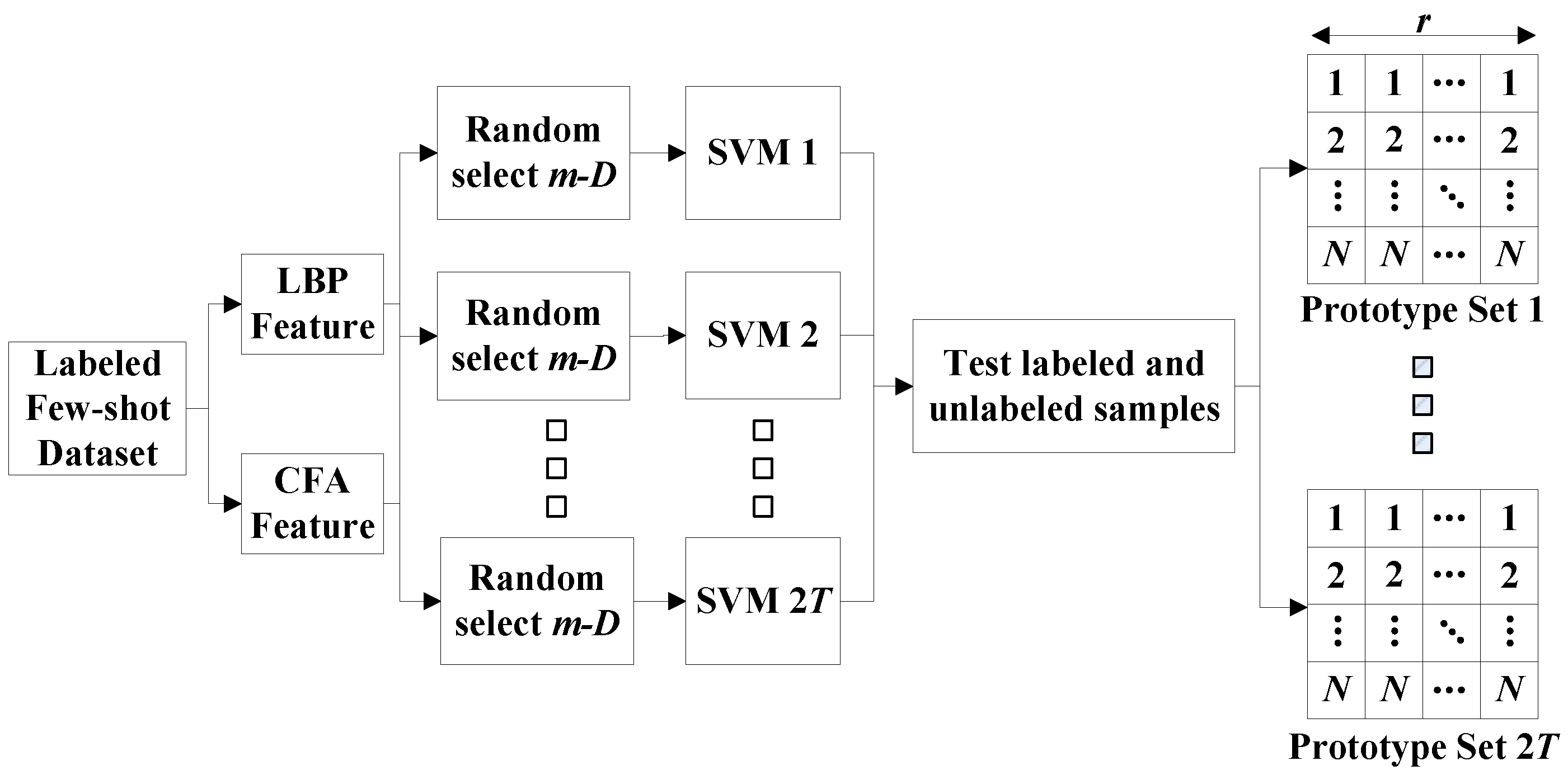
  • We propose an ensemble learning projection method based on prototype set construction (PCEP). This method extracts multiple image features through semi-supervised learning, realizes prototype set construction and makes full use of the information of few-shot samples.
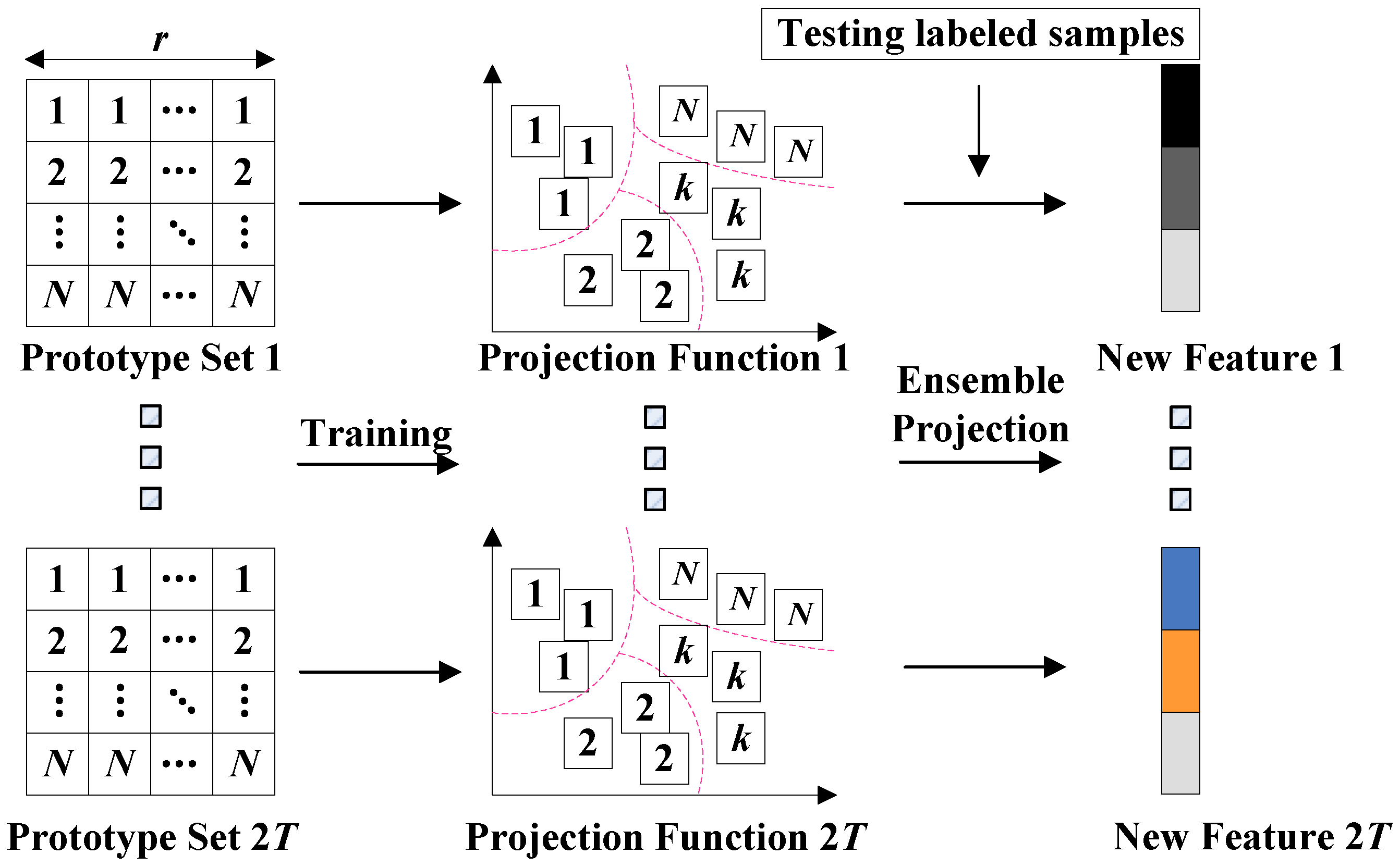
  • We use the prototype sets to carry out ensemble learning projections and realize the transformation from image features to probability features.
  • We introduce the ensemble learning voting strategy to obtain the final classification results. Our comprehensive experimental results show that this method is superior to many recent methods in a few-shot scenario.

2. Related Work

In this section, we review the existing literature in the field of source camera identification. The main research problem of source camera identification is how to effectively distinguish the brand, model or individual of the device used for image acquisition. In this study, we mainly conduct camera model identification.
The primary task of researching source camera identification is to have a clear understanding of camera imaging principles, so as to extract effective features and realize the mapping between multimedia images and physical devices. Researchers have found that a scheme based on sensor pattern noise [21,22,23] is a very effective means for source forensics. Sensor pattern noise is generated by some inevitable manufacturing defects in the process of sensor manufacturing. It is independent and can be used to identify different devices of the same brand. Lukas et al. [21] first applied the use of pattern noise in the image sensor as the inherent fingerprint of the device in source camera identification. In order to reduce the impact of image content, Li et al. [24] arranged images according to different image content, and assigned different weight coefficients to the pattern noise at different levels, which effectively suppressed the image content information in the texture area. Kang et al. [25] could better interpolate images by using the content adaptive interpolation algorithm, especially to retain the edge information. In this way, the residual image obtained by difference could better reduce the impact of the edge. The study in [26] made new improvements on the basis of a local discrete cosine transform filter, making it more difficult for the filtered image to maintain its original image quality, so that the residual image was less affected by the image content. The experiments in [22,27] used the Fourier spectrum of mode noise to suppress the peak value in the spectrum and reduce the impact of periodicity. In recent years, in addition to the traditional methods based on sensor noise, there have been many methods of image forensics using a neural network. Liu et al. [28] proposed an efficient patch-level source camera identification method based on a convolutional neural network. Hui et al. [29] proposed a multi-scale feature fusion network (MSFFN) to boost the sensor-based source camera identification attribution. Zhang et al. [30] proposed an effective source camera identification scheme based on a Multi-Scale Expected Patch Log Likelihood (MSEPLL) denoising algorithm. Their experimental results show that the selection of small image block samples also has a great impact on actual source classification results.
All of the above experiments, however, were performed in a training environment with sufficient labeled samples. When there are insufficient training samples, the performance of the above algorithms become greatly reduced. Common methods used to address few-shot problems include data augmentation, semi-supervised learning, etc. The data augmentation method aims to enhance the diversity of samples and provide sufficient feature information by enhancing data in the sample space or feature space. At the same time, semi-supervised learning uses unlabeled samples to strengthen the training model and make it conform to the clustering hypothesis. Tan et al. [31] studied camera model identification with limited samples, and used more abundant features to solve the problem. Boney et al. [32] proposed that the parameters of embedded functions could be adjusted with unlabeled data, and the parameters of classifiers could be adjusted with labeled data. Hou et al. [20] proposed a cross-attention network, which uses the attention mechanism and idea of iteration to make full use of the sample information in the query set to achieve data enhancement. Schwartz et al. [33] proposed a Delta encoder that could synthesize new samples in the feature space. Chen et al. [34] proposed a bidirectional network called TriNet, taking advantage of semantic information of category labels and mapping sample features to label semantic space for data enhancement, and then mapping this back to the sample feature space. The above methods provide feasible solutions for practical application scenarios with insufficient data, and also provided the inspiration for our work.

3. The PCEP Method

In order to build a more reliable model for camera model identification in the case of few-shot samples, we proposed an ensemble learning projection method based on prototype set construction, called PCEP. The specific approach is shown in Algorithm 1. Firstly, we extracted multiple image features from few-shot datasets to complete the pre-training of a variety of classifiers. Then, we introduced semi-supervised learning to test all image samples, and these samples with higher posterior probability were selected to form prototype sets. Subsequently, we used these prototype sets to retrain SVM classifiers, and took the posterior probability of each image sample belonging to each class as the final projection vector, namely, new classification features, and used new features to train multiple weak classifiers. Finally, we obtained the classification results through ensemble learning voting. The details of each step of the methodology are described in the following section.
Algorithm 1:Prototype construction with ensemble projection (PCEP)
Symbols:
    S l : Labeled sample set; S u : Unlabeled sample set; S f e w : Labeled few-shot dataset; p: Posterior probability of the sample; P: Prototype set; E: Ensemble projection vector
Process:
   1. Extract CFA and LBP features from S f e w ;
   2. Train SVM classifiers based on partial feature information;
   3. Construct prototype sets:
   for s S l , S u do
      Put s into SVM classifiers to obtain the posterior probability p
   end for
   Sort p in descending order and take the first r entries to form prototype sets P
   4. Obtain ensemble projection features:
   for  i P  do
      Train the projection function based on i
      Put s ( s S l ) into the projection function to obtain the ensemble projection vector E
   end for
   5. Obtain the final classification result:
   for  j E  do
      Train the weak classifier based on j
      Put s ( s S u ) into the weak classifier to obtain the sub-classification result
   end for
   Obtain the final classification result using ensemble voting strategy.

3.1. Constructing Prototype Set

In order to make full use of the information of few-shot datasets and obtain more prior information in the case of limited samples, we introduced two kinds of image features and implemented the construction of prototype sets according to semi-supervised theory.
The PCEP method introduces color filter array (CFA) features and local binary pattern (LBP) features, which have different generalization capabilities. The invariance and equivariance of the two kinds of features complement each other to realize the optimal utilization of few-shot datasets in SCI. For CFA features, we calculated the interpolation coefficients on three color channels. According to the method in [35], a total of ( ( 2 k + 1 ) 2 1 ) × 5 = 240 interpolation coefficients were obtained. The mean and variance of 240 dimensional CFA interpolation coefficients were integrated into 480 dimensional CFA features. LBP is a local operator that describes the textural features of an image, and the feature extraction framework of one color channel is shown in Figure 1. It includes a prediction error domain, spatial domain and wavelet transform domain. The radius of the LBP operator we adopted was 1, so there were 2 8 = 256 modes of LBP features for 8 neighborhood pixels. According to the dimension reduction model proposed by Ojala et al. [5], we extracted 59-dimensional LBP features from the three domains. In addition, the image post-processing algorithms corresponding to the red and blue channels were the same in most cases, with only one needing to be selected. Therefore, from the red and green channels of the original image, we extracted the LBP features in the spatial domain, prediction error domain and wavelet transform domain. Finally, we obtained 59 × 3 × 2 = 354 dimensional LBP features.
According to prototype set theory [36], there are some items closer to the center than others in the same scope. This fully proves that, among many unlabeled samples, some samples are always more likely to belong to a certain class than others. Therefore, we can calibrate the pseudo-labels for these samples, and further utilize their information to obtain higher classification accuracy. In the actual operation of this study, we selected multiple groups ( 2 T ) of labeled and unlabeled samples closer to the center from different angles to form multiple prototype sets. The specific construction of the prototype set is shown in Figure 2. In this paper, we first extracted LBP and CFA features from all labeled samples, then randomly selected m-dimensional (abbreviated as m D ) features to train several N-class classifiers. Therefore, a total of 2 T group classifiers were trained; that is, LBP features corresponded to T group classifiers and CFA features corresponded to T group classifiers. Then, in a semi-surpervised manner, all samples were passed through the classifiers to obtain the posterior probability belonging to each class. All samples were sorted by the posterior probability (large to small), and the top r samples in each class were selected to construct prototype sets. Finally, we had 2 T prototype sets.
In addition, if some samples belonging to each class have similar posterior probabilities, it is considered that these samples do not provide any available information. In this study, we treated these samples as noise samples. According to information theory, if the probability of a sample belonging to each class is equal, maximum entropy can be obtained. The larger the entropy, the closer the sample is to the noise sample. Therefore, we discarded some samples according to their calculated entropy. The calculation formula of entropy is as follows:
e n t r o p y = N i = 1 p i log 2 p i
In Equation (1), p i indicates the possibility of a sample belonging to class i.

3.2. Training Ensemble Projection Features and Voting Classification

According to the 2 T prototype sets, we obtained the ensemble projection features by training. The specific process is shown in Figure 3. Different colors in the new feature correspond to different classes of posterior probabilities. Each prototype set was used as a new training set to train a new SVM classifier, thus obtaining 2 T classifiers, which were called projection functions. Then, labeled training samples are were mapped using the projection functions to obtain the posterior probabilities, which were saved as new features. As we used LBP and CFA features to construct the prototype sets, after projection, we had LBP projection vectors and CFA projection vectors.
The above projection vectors were mapped by weak classifiers, which were obtained by partial dimensions of sample features, so the idea of ensemble learning was introduced. Ensemble learning [37] aims to integrate all sub-learning results and improve accuracy. As shown in Figure 4, according to ensemble learning, we used the projection vectors to train several classification models. Accordingly, we placed unlabeled samples and obtained the test results. Then, according to the voting method of ensemble learning, we obtained the final results.

4. Experiments

In this section, we first introduce the experimental settings. Then, we evaluate the effectiveness of PCEP in few-shot scenarios and analyze the experimental results in detail.

4.1. Experimental Settings

In this study, we tested the performance of the PCEP method on three public databases: Dresden [38], VISION [39] and SOCRatES databases [40]. We selected 16 different classes of equipment in the Dresden database, 10 different classes of equipment in the VISION database and 10 different classes of equipment in the SOCRatES database. Among them, the number of training samples was limited, ranging from 5, 10, 15, 20 and 25 samples for each class. The test set consisted of 150 samples for each class. The specific information of the selected equipment is shown in Table 1, Table 2 and Table 3.

4.2. Experimental Results and Analysis

In this study, the baseline method using only LBP features was named LBP-SVM, and the method using only CFA features was named CFA-SVM. The baseline using dual features was named multi-SVM. After using the PCEP method, the method using only LBP features, only CFA features and dual features were named LBP-PCEP, CFA-PCEP and multi-PCEP, respectively.
In order to get closer to a real few-shot scenario, we set the number of training samples for each class L as 5, 10, 15, 20 and 25. To determine the number of prototype sets T and number of samples for each class in the prototype set r on the experimental effects, we conducted detailed experiments on each database based on the above-mentioned L. It is worth noting that in order to ensure the stability of the experimental results, we conducted 10 random training and testing sessions for all experiments, and averaged the results for the final experimental results.
We tested the effect of the number of prototype sets T on the experimental results of the three databases, and the experimental results are shown in Figure 5. It can be observed that with an increase in T, classification accuracy is improved, which proves that the larger the number of prototype sets T, the greater the number of ensemble classifiers, and the higher the accuracy. Therefore, after comprehensive consideration, we finally set T to be 50. In addition, the number of training samples for each class L also affected the stability of performance. When L is small, classification accuracy is low and fluctuates greatly.
We also carried out experiments on the number of samples for each class in the prototype set r. As shown in Figure 6, the more samples of each class, the higher the classification accuracy. Judging from the results of the multiple databases, the number of samples for each class in the prototype sets r had a greater impact on the experimental results than the number of prototype sets T. However, as r increased, the rise in accuracy began to slow down. In an actual judicial evidence scenario, the number of unlabeled samples for semi-supervised learning is usually not large, so we decided to set r to 50.
We compared the baseline method with the proposed PCEP method on the Dresden database, and the results are shown in Table 4. In this paper, the highest value in the same case is expressed in bold, and the following is similar. It was observed that multi-PCEP achieved the best performance. Especially in the case of L = 5, compared with the corresponding SVM method, the accuracy of the three PCEP methods (LBP-PCEP, CFA-PCEP and multi-PCEP) was greatly improved, being 3.5%, 18.08% and 12.79%, respectively. In addition, as L increases, the improvements in classification accuracy of the various methods tend to be subtle, so the experimental results when L was greater than 25 are not listed in this paper. The results fully demonstrated that the multi-PCEP method could optimize the utilization of few-shot samples and had the highest accuracy rate of source camera identification among all the methods. These results also demonstrate the effectiveness of new features generated by the multi-PCEP method and ensemble learning method in the optimization and utilization of few-shot samples.
To verify the generalization of our proposed method, we conducted experiments on the VISION and SOCRatES databases; the experimental results are shown in Table 5 and Table 6. The PCEP method achieved the best performance on both databases. Especially in the case of small L, PCEP significantly improved the accuracy compared with the three baseline methods. For the VISION database, when L = 5, the multi-PCEP method improved accuracy by 24.98%, 34.8% and 2.14% compared with LBP-SVM, CFA-SVM and multi-SVM, respectively. On the SOCRatES database, the multi-PCEP method improved accuracy by 23.03%, 41.48% and 11.93% compared with LBP-SVM, CFA-SVM and multi-SVM, respectively.
In order to verify the superiority of our PCEP method, we compared it with other existing methods, including EP [31], the deep Siamese network [41], multi-DS [42], and MTDEM [43]. The comparison experimental results are shown in Table 7. We reselected 14 (in Dresden database), 11 (in VISION database) and 10 (in SOCRatES database) camera model classes with 10 training samples per class to keep consistent with the comparison methods. The comparison experimental results showed that our method performed better than other recent methods in the same experimental setup.
In addition, aiming to draw an analogy with the method based on the deep Siamese network, we verified the impact of the number of camera model classes selected from the databases on classification accuracy. The number of camera model classes in the Dresden database varied from 14 to 27 (the whole dataset), and the number of classes in the VISION database varied from 11 to 35 (the whole dataset). The experimental results are shown in Figure 7. The experimental results showed that, as the number of models increased, the accuracy gradually decreased. Our results followed the same trend as the method based on the deep Siamese network.
In terms of time complexity, our approach also had significant advantages over deep learning-based approaches.This is because our approach does not require a large number of complex iterative calculations. For example, in the case of 14 classes, each training round of the deep Siamese network method takes several hours, and multiple rounds are needed to obtain better results, so the total training time is very long. The specific running time of the PCEP method includes two parts: feature extraction and classification training. When extracting features from a labeled few-shot dataset, it takes about 12 s to extract CFA features and about 21 s to extract LBP features for each image. Although the training time of our method varies depending on the number of classes and the number of samples per class, it is only tens to hundreds of seconds. We conducted time complexity experiments for two databases, where 16 classes were selected from the Dresden database and 10 classes were selected from the VISION database. The specific experimental table is shown in Table 8. Therefore, our method is more suitable for fast analyses in practical situations.
Finally, we conducted a confusion matrix experiment on the three databases (Dresden, VISION and SOCRatES databases, in that order) with L = 25, and the experimental results are shown in Table 9, Table 10 and Table 11. The correct classification ratio in the confusion matrix is expressed in bold, and the short dash in the table represents a classification probability below 0.01%. On the Dresden database, we found that the classification accuracy of the SD1 and SD3 cameras were only 55.65 and 51.42%, respectively. It can be seen from the results that these two models are confused with each other in the identification of image source, which is the similar to results of the previous LBP-SVM and CFA-SVM methods. They are also often confused in classification, that is, the same phenomenon that is being addressed in this paper. The reason is that the two types of cameras adopt similar image post-processing methods, which makes their images difficult to differentiate in classification. According to the above confusion matrices, it was found that the multi-PCEP method is applicable to different databases; that is, it is effective in different databases for camera model identification of few-shot samples.

5. Discussion

Aiming to solve the problem of few-shot sample classification in source camera identification, we proposed an ensemble learning projection method based on prototype set construction (PCEP). We adopted semi-supervised theory to further optimize the few-shot sample features, which effectively increased the available information and helped build a more comprehensive and strong supervision model through ensemble learning. Empirical results demonstrated that the PCEP method could effectively improve classification accuracy in few-shot scenarios, and showed higher performance than other existing methods. In future work, we aim to try more feature extraction methods, and integrate different feature extraction methods inspired by MU-LTP and CLQP. Secondly, in an era of deep learning, it is important to consider trying to combine the features learned by CNN with classic features to improve overall performance. In addition, determining how to ensure reliable performance in cases of extreme few-shot samples (i.e., the number of samples of each class is less than 5) is another hot topic of our work.

Author Contributions

Conceptualization, B.W. and F.Y.; methodology, F.Y.; validation, F.Y., Y.M. and H.Z.; formal analysis, B.W.; investigation, F.Y. and J.H.; data curation, W.Z.; writing—original draft preparation, F.Y.; writing—review and editing, B.W.; visualization, F.Y.; supervision, B.W. All authors have read and agreed to the published version of the manuscript.

Funding

This work is supported by the National Natural Science Foundation of China (No. U1936117, 62106037 and 62076052), the Science and Technology Innovation Foundation of Dalian (No. 2021JJ12GX018), the Application Fundamental Research Project of Liaoning Province (2022JH2/101300262), the Open Project Program of the National Laboratory of Pattern Recognition (NLPR) (No. 202100032) and Fundamental Research Funds for the Central Universities (DUT21GF303, DUT20TD110, DUT20RC(3)088).

Data Availability Statement

Data will be made available upon reasonable request.

Conflicts of Interest

The authors declare no conflict of interest.

Abbreviations

The following abbreviations are used in this manuscript:
PCEPPrototype construction with ensemble projection
SCISource camera identification
SVMSupport vector machine
CFAColor filter array
LBPLocal binary pattern

References

  1. Fridrich, A.J.; Soukal, B.D.; Lukáš, A.J. Detection of copy-move forgery in digital images. In Proceedings of the Digital Forensic Research Workshop, Cleveland, OH, USA, 6–8 August 2003. [Google Scholar]
  2. Ho, A.T.; Li, S. Handbook of Digital Forensics of Multimedia Data and Devices; John Wiley & Sons: Hoboken, NJ, USA, 2015. [Google Scholar]
  3. Sandoval Orozco, A.L.; Corripio, J.R.; García Villalba, L.J.; Hernández Castro, J.C. Image source acquisition identification of mobile devices based on the use of features. Multimed. Tools Appl. 2016, 75, 7087–7111. [Google Scholar] [CrossRef]
  4. Pietikäinen, M.; Ojala, T.; Xu, Z. Rotation-invariant texture classification using feature distributions. Pattern Recognit. 2000, 33, 43–52. [Google Scholar] [CrossRef]
  5. Ojala, T.; Pietikainen, M.; Maenpaa, T. Multiresolution gray-scale and rotation invariant texture classification with local binary patterns. IEEE Trans. Pattern Anal. Mach. Intell. 2002, 24, 971–987. [Google Scholar] [CrossRef]
  6. Tan, X.; Triggs, B. Enhanced Local Texture Feature Sets for Face Recognition Under Difficult Lighting Conditions. IEEE Trans. Image Process. 2010, 19, 1635–1650. [Google Scholar] [PubMed]
  7. Guo, Z.; Zhang, L.; Zhang, D. A completed modeling of local binary pattern operator for texture classification. IEEE Trans. Image Process. 2010, 19, 1657–1663. [Google Scholar] [PubMed]
  8. Fekri-Ershad, S.; Ramakrishnan, S. Cervical cancer diagnosis based on modified uniform local ternary patterns and feed forward multilayer network optimized by genetic algorithm. Comput. Biol. Med. 2022, 144, 105392. [Google Scholar] [CrossRef] [PubMed]
  9. Pourkaramdel, Z.; Fekri-Ershad, S.; Nanni, L. Fabric defect detection based on completed local quartet patterns and majority decision algorithm. Expert Syst. Appl. 2022, 198, 116827. [Google Scholar] [CrossRef]
  10. Mahmmod, B.M.; Abdulhussain, S.H.; Suk, T.; Hussain, A. Fast computation of Hahn polynomials for high order moments. IEEE Access 2022, 10, 48719–48732. [Google Scholar] [CrossRef]
  11. Wang, Y.X.; Girshick, R.; Hebert, M.; Hariharan, B. Low-shot learning from imaginary data. In Proceedings of the IEEE conference on computer vision and pattern recognition, Salt Lake City, UT, USA, 18–22 June 2018. [Google Scholar]
  12. Hu, X.; Yang, Z.; Liu, G.; Liu, Q.; Wang, H. Virtual label expansion-Highlighted key features for few-shot learning. In Proceedings of the 2021 International Joint Conference on Neural Networks, Shenzhen, China, 18–22 July 2021. [Google Scholar]
  13. Wang, B.; Wu, S.; Wei, F.; Wang, Y.; Hou, J.; Sui, X. Virtual sample generation for few-shot source camera identification. J. Inf. Secur. Appl. 2022, 66, 103153. [Google Scholar] [CrossRef]
  14. Khodadadeh, S.; Boloni, L.; Shah, M. Unsupervised meta-learning for few-shot image classification. Adv. Neural Inf. Process. Syst. 2019, 32, 10132–10142. [Google Scholar]
  15. Xu, H.; Wang, J.; Li, H.; Ouyang, D.; Shao, J. Unsupervised meta-learning for few-shot learning. Pattern Recognit. 2021, 116, 107951. [Google Scholar] [CrossRef]
  16. Huang, K.; Geng, J.; Jiang, W.; Deng, X.; Xu, Z. Pseudo-loss confidence metric for semi-supervised few-shot learning. In Proceedings of the IEEE/CVF International Conference on Computer Vision, Montreal, QC, Canada, 10–17 October 2021. [Google Scholar]
  17. Ling, J.; Liao, L.; Yang, M.; Shuai, J. Semi-Supervised Few-Shot Learning via Multi-Factor Clustering. In Proceedings of the IEEE/CVF Conference on Computer Vision and Pattern Recognition, New Orleans, LA, USA, 18–24 June 2022. [Google Scholar]
  18. Zhang, B.; Ye, H.; Yu, G.; Wang, B.; Wu, Y.; Fan, J.; Chen, T. Sample-Centric Feature Generation for Semi-Supervised Few-Shot Learning. IEEE Trans. Image Process. 2022, 31, 2309–2320. [Google Scholar] [CrossRef] [PubMed]
  19. Gidaris, S.; Komodakis, N. Dynamic few-shot visual learning without forgetting. In Proceedings of the IEEE Conference on Computer Vision and Pattern Recognition, Salt Lake City, UT, USA, 18–22 June 2018. [Google Scholar]
  20. Hou, R.; Chang, H.; Ma, B.; Shan, S.; Chen, X. Cross attention network for few-shot classification. Adv. Neural Inf. Process. Syst. 2019, 32, 4005–4016. [Google Scholar]
  21. Lukas, J.; Fridrich, J.; Goljan, M. Digital camera identification from sensor pattern noise. IEEE Trans. Inf. Forensics Secur. 2006, 1, 205–214. [Google Scholar] [CrossRef]
  22. Kang, X.; Li, Y.; Qu, Z.; Huang, J. Enhancing source camera identification performance with a camera reference phase sensor pattern noise. IEEE Trans. Inf. Forensics Secur. 2011, 7, 393–402. [Google Scholar] [CrossRef]
  23. Cozzolino, D.; Gragnaniello, D.; Verdoliva, L. Image forgery localization through the fusion of camera-based, feature-based and pixel-based techniques. In Proceedings of the 2014 IEEE International Conference on Image Processing (ICIP), Paris, France, 27–30 October 2014. [Google Scholar]
  24. Li, R.; Li, C.T.; Guan, Y. A reference estimator based on composite sensor pattern noise for source device identification. In Proceedings of the Media Watermarking, Security, and Forensics, San Francisco, CA, USA, 2 February 2014. [Google Scholar]
  25. Kang, X.; Chen, J.; Lin, K.; Anjie, P. A context-adaptive SPN predictor for trustworthy source camera identification. EURASIP J. Image Video Process. 2014, 2014, 1–11. [Google Scholar] [CrossRef]
  26. Lawgaly, A.; Khelifi, F. Sensor pattern noise estimation based on improved locally adaptive DCT filtering and weighted averaging for source camera identification and verification. IEEE Trans. Inf. Forensics Secur. 2016, 12, 392–404. [Google Scholar] [CrossRef]
  27. Lin, X.; Li, C.T. Preprocessing reference sensor pattern noise via spectrum equalization. IEEE Trans. Inf. Forensics Secur. 2015, 11, 126–140. [Google Scholar] [CrossRef]
  28. Liu, Y.; Zou, Z.; Yang, Y.; Law, N.F.B.; Bharath, A.A. Efficient source camera identification with diversity-enhanced patch selection and deep residual prediction. Sensors 2021, 21, 4701. [Google Scholar] [CrossRef] [PubMed]
  29. Hui, C.; Jiang, F.; Liu, S.; Zhao, D. Source Camera Identification with Multi-Scale Feature Fusion Network. In Proceedings of the 2022 IEEE International Conference on Multimedia and Expo, Taipei, Taiwan, 18–22 July 2022. [Google Scholar]
  30. Zhang, W.N.; Liu, Y.X.; Zou, Z.Y.; Zang, Y.L.; Yang, Y.; Law, B.N.F. Effective source camera identification based on MSEPLL denoising applied to small image patches. In Proceedings of the 2019 Asia-Pacific Signal and Information Processing Association Annual Summit and Conference (APSIPA ASC), Lanzhou, China, 18–21 November 2019. [Google Scholar]
  31. Tan, Y.; Wang, B.; Li, M.; Guo, Y.; Kong, X.; Shi, Y. Camera source identification with limited labeled training set. In Proceedings of the International Workshop on Digital Watermarking, Tokyo, Japan, 7–10 October 2015. [Google Scholar]
  32. Boney, R.; Ilin, A. Semi-supervised few-shot learning with MAML. In Proceedings of the 6th International Conference on Learning Representations, ICLR 2018, Vancouver, BC, Canada, 30 April–3 May 2018. [Google Scholar]
  33. Schwartz, E.; Karlinsky, L.; Shtok, J.; Harary, S.; Marder, M.; Kumar, A.; Feris, R.; Giryes, R.; Bronstein, A. Delta-encoder: An effective sample synthesis method for few-shot object recognition. In Proceedings of the Advances in Neural Information Processing Systems, Montreal, QB, Canada, 3–8 December 2018. [Google Scholar]
  34. Chen, Z.; Fu, Y.; Zhang, Y.; Jiang, Y.G.; Xue, X.; Sigal, L. Semantic feature augmentation in few-shot learning. arXiv 2018, arXiv:1804.05298. [Google Scholar]
  35. Gardenfors, P. Conceptual Spaces: The Geometry of Thought; MIT Press: Cambridge, MA, USA, 2004. [Google Scholar]
  36. Rosch, E.; Lloyd, B.B. Cognition and Categorization; Urban Ministried Inc.: Calumet City, IL, USA, 1978. [Google Scholar]
  37. Dai, D.; Van Gool, L. Ensemble projection for semi-supervised image classification. In Proceedings of the IEEE International Conference on Computer Vision, Sydney, Australia, 1–8 December 2013. [Google Scholar]
  38. Gloe, T.; Böhme, R. The ‘Dresden Image Database’ for benchmarking digital image forensics. In Proceedings of the 2010 ACM Symposium on Applied Computing, Sierre, Switzerland, 22–26 March 2010. [Google Scholar]
  39. Shullani, D.; Fontani, M.; Iuliani, M.; Al Shaya, O.; Piva, A. VISION: A video and image dataset for source identification. EURASIP J. Inf. Secur. 2017, 2017, 1–16. [Google Scholar] [CrossRef]
  40. Galdi, C.; Hartung, F.; Dugelay, J.L. SOCRatES: A Database of Realistic Data for Source Camera Recognition on Smartphones. In Proceedings of the 8th International Conference on Pattern Recognition Applications and Methods, Prague, Czech Republic, 19–21 February 2019. [Google Scholar]
  41. Sameer, V.U.; Naskar, R. Deep siamese network for limited labels classification in source camera identification. Multimed. Tools Appl. 2020, 79, 28079–28104. [Google Scholar] [CrossRef]
  42. Wang, B.; Hou, J.; Ma, Y.; Wang, F.; Wei, F. Multi-DS Strategy for Source Camera Identification in Few-Shot Sample Data Sets. Secur. Commun. Netw. 2022, 2022, 8716884. [Google Scholar] [CrossRef]
  43. Wu, S.; Wang, B.; Zhao, J.; Zhao, M.; Zhong, K.; Guo, Y. Virtual sample generation and ensemble learning based image source identification with small training samples. Int. J. Digit. Crime Forensics 2021, 13, 34–46. [Google Scholar] [CrossRef]
Figure 1. LBP feature extraction framework for one color channel.
Mathematics 11 00803 g001
Figure 2. Pipeline of constructing prototype set.
Mathematics 11 00803 g002
Figure 3. Training ensemble projection functions used to obtain new features of images.
Mathematics 11 00803 g003
Figure 4. Ensemble learning to integrate all sub-learning results and increase the diversity of projection vectors.
Mathematics 11 00803 g004
Figure 5. Accuracy rate versus the number of prototype sets T for the three databases: (a) Dresden, (b) VISION, and (c) SOCRatES.
Mathematics 11 00803 g005aMathematics 11 00803 g005b
Figure 6. Accuracy rate versus the number of samples for each class in the prototype set r on the three databases: (a) Dresden, (b) VISION, and (c) SOCRatES.
Mathematics 11 00803 g006aMathematics 11 00803 g006b
Figure 7. Effect of number of classes on accuracy in two databases: (a) Dresden and (b) VISION.
Mathematics 11 00803 g007
Table 1. Dataset in experiments (Dresden).
Camera ModelAbbr.Camera ModelAbbr.
Canon_Ixus70C1Panasonic_DMC-FZ50P1
Casio_EX-Z150C2Praktica_DCZ5.9P2
FujiFilm_FinePixJ50F1Rollei_RCP-7325XSR1
Kodak_M1063K1Samsung_L74wideSL1
Nikon_CoolPixS710N1Samsung_NV15SN1
Nikon_D70N2Sony_DSC-H50SD1
Nikon_D200N3Sony_DSC-T77SD2
Olympus_mju_1050SWO1Sony_DSC-W170SD3
Table 2. Dataset in experiments (VISION).
Camera ModelAbbr.Camera ModelAbbr.
Samsung_GalaxyS3Sa1Apple_iPhone6Ap3
Apple_iphone4sAp1Lenovo_P70ALe1
Huawei_P9Hu1Samsung_GalaxyTab3Sa2
LG_D290Lg1Apple_iPhone4Ap4
Apple_iPhone5cAp2Microsoft_Lumia640LTEMi1
Table 3. Dataset in experiments (SOCRatES).
Camera ModelAbbr.Camera ModelAbbr.
Apple iPhone 5sA1LG G3L1
Apple iPhone 6A2Motorola Moto GM1
Apple iPhone 6sA3Samsung Galaxy A3SG1
Apple iPhone 7A4Samsung GalaxyS5SG2
Asus Zenfone 2As1Samsung Galaxy S7 EdgeSG3
Table 4. Average accuracy of source camera identification on “Dresden Database”.
Method (%)The Number of Training Samples per Class (L)
510152025
LBP-SVM45.6471.2478.9783.2985.45
CFA-SVM49.7569.9978.6782.6884.89
Multi-SVM64.3678.6481.6784.2686.13
LBP-PCEP49.1468.6278.4182.0184.17
CFA-PCEP67.8377.1580.3681.9282.79
Multi-PCEP77.1585.2687.6288.5089.09
Table 5. Average accuracy of source camera identification on “VISION Database”.
Method (%)The Number of Training Samples per Class (L)
510152025
LBP-SVM49.9680.3485.9588.3689.10
CFA-SVM40.1462.7581.1486.1087.11
Multi-SVM72.8076.7182.3682.8183.42
Multi-PCEP74.9483.9986.5988.4690.51
Table 6. Average accuracy of source camera identification on “SOCRatES Database”.
Method (%)The Number of Training Samples per Class (L)
510152025
LBP-SVM38.5667.2476.0679.6781.78
CFA-SVM20.1157.1366.7674.0477.06
Multi-SVM49.6657.5367.4573.1375.81
Multi-PCEP61.5975.9478.6380.2081.81
Table 7. Camera identification accuracy compared with previous methods.
Method (%)DresdenVISIONSOCRatES
EP [31]73.8479.9463.91
MTDEM [43]75.1680.4964.84
Deep Siamese Network [41]85.3075.20\
Multi-DS [42]86.0885.5667.00
Multi-PCEP87.0684.8475.94
Table 8. Time complexity of the PCEP method.
Database(s)L (the Number of Training Samples per Class)
510152025
Dresden (16 classes)155247406596853
VISION (10 classes)62103165238341
Table 9. Average confusion matrix obtained by 20 repetitions of SVM classification (Dresden database).
C1C2F1K1N1N2N3O1P1P2R1S1S2SD1SD2SD3
C199.20.2-------0.6------
C20.895.9-0.2--0.1-0.2--2.8----
F10.1-91.7-0.2-0.5-0.10.23.81.80.4-1.2-
K10.52.30.292.10.13.10.3-0.10.6-0.4-0.1-0.2
N11.71.80.1-92.40.30.4--0.70.22.4----
N20.31.0-1.40.490.63.7--1.00.20.2-0.4-0.8
N3--0.31.2-5.492.3---0.2-0.6---
O1--0.1--0.20.996.5---2.3----
P10.20.5-0.5--0.30.295.8--2.00.5---
P21.50.4-0.30.20.40.5-1.093.60.10.70.50.3-0.5
R1-0.14.8--0.20.3-0.10.191.72.30.4---
S1-2.31.3---0.40.10.10.70.394.70.1---
S20.50.20.3---0.1--1.81.00.595.20.2-0.2
SD10.60.8-0.1-1.30.8--0.3--0.655.70.439.4
SD2-1.20.3--0.20.2---0.10.9-0.296.70.2
SD3-0.3-0.1-1.80.3--0.50.2-0.445.0-51.4
Table 10. Average confusion matrix obtained by 20 repetitions of SVM classification (VISION database).
Sa1Ap1Hu1Lg1Ap2Ap3Le1Sa2Ap4Mi1
Sa190.5-1.62.1-3.10.22.5--
Ap10.276.51.22.811.73.91.1-0.52.1
Hu10.20.886.54.70.16.11.0--0.6
Lg1--1.795.10.80.71.5--0.2
Ap2-3.90.93.388.61.30.30.5-1.2
Ap30.31.21.10.94.090.50.30.4-1.3
Le1---3.70.80.194.8--0.6
Sa20.5-0.91.60.20.2-96.6--
Ap4---0.70.10.1--99.1-
Mi1-6.60.23.00.31.8--1.087.1
Table 11. Average confusion matrix obtained by 20 repetitions of SVM classification (SOCRatES database).
A1A2A3A4As1L1M1S1S2S3
A182.76.34.00.92.40.80.1-2.8-
A26.474.86.54.21.80.43.21.10.80.8
A35.48.175.87.21.60.11.40.10.10.2
A43.95.79.273.73.30.21.80.81.4-
As14.00.42.43.285.60.31.10.72.3-
L10.30.8-4.55.183.13.21.02.0-
M10.20.62.64.56.61.481.30.62.10.1
S1-1.20.50.42.40.10.891.21.91.5
S24.70.81.02.22.42.71.90.682.90.8
S31.00.71.61.44.30.81.21.60.387.1
Disclaimer/Publisher’s Note: The statements, opinions and data contained in all publications are solely those of the individual author(s) and contributor(s) and not of MDPI and/or the editor(s). MDPI and/or the editor(s) disclaim responsibility for any injury to people or property resulting from any ideas, methods, instructions or products referred to in the content.

