Equation-Based Modeling vs. Agent-Based Modeling with Applications to the Spread of COVID-19 Outbreak

Abstract

In this paper, we explore two modeling approaches to understanding the dynamics of infectious diseases in the population: equation-based modeling (EBM) and agent-based modeling (ABM). To achieve this, a comparative study of these approaches was conducted and we highlighted their advantages and disadvantages. Two case studies on the spread of the COVID-19 pandemic were carried out using both approaches. The results obtained show that differential equation-based models are faster but still simplistic, while agent-based models require more machine capabilities but are more realistic and very close to biology. Based on these outputs, it seems that the coupling of both approaches could be an interesting compromise.

1. Introduction

COVID-19 (SARS-CoV-2) is a devastating disease that has spread around the world since the last quarter of 2019. Although the exact origin of the virus is still unknown, the first officially recognized outbreak was reported in Wuhan, China in November 2019. This disease is a deadly pandemic that is transmitted from an animal (host) to another one (intermediate host) or from an intermediate host to humans [1]. Human-to-human transmission occurs mainly through respiratory droplets and aerosolization when a person breathes in the same enclosed space or in close proximity to other people. Transmission increases in poorly ventilated indoors and when the infected person coughs, sneezes, talks, or sings [2,3]. A sudden loss of smell (anosmia), whether or not associated with a loss of taste (ageusia), is a relatively frequent manifestation and the revealing origin of SARS-CoV-2 infection. Other common symptoms may be fever, cough, the difficulty of breathing, chills, muscle aches or sore throat. Symptoms may occur from the second day after the contamination to the 14th one. The novel coronavirus might cause a moderate or severe form of infection. The severe form involves complications such as pneumonia or death of the infected person. A specific category known as “highly comorbid individuals” is considered as the class of individuals with high risk of having the severe form of COVID-19. This category concerns people of all ages with underlying health problems, especially if those problems are poorly controlled, including people with chronic lung disease [4] or moderate to severe asthma, heart disease, weakened immune system, severe obesity (body mass index of 40 or more), diabetes, chronic kidney disease, especially with dialysis, and liver disease.

The spread of COVID-19 is a very complex phenomenon that draws the attention of many researchers. To overcome the pandemic of COVID-19, it is advisable to study and model it as a complex system that requires a solution in the form of modeling simulation for its understanding. In the literature, complex systems have been mainly studied by means of equation-based models (EBM) and agent-based models (ABM).

The first point of view (EBM) is based on mathematical modeling. In this direction, ref [5] presented a general model of epidemic spread to understand the timing of transmission. In [6], the authors studied, with the aid of mathematical models, the infection force of the hepatitis C virus among drug users in France. In [7], a mathematical model of the COVID-19 outbreak with three forms of infections (benign, respiratory, and reanimation forms) is proposed. In [8], complex systems, such as the spread of tuberculosis, are solved by means of hybrid stochastic modeling and computer simulations. In their study, ref [9] established a model of differential equations with piecewise constant arguments in order to explore the spread of COVID-19. A formulation of a stochastic susceptible-infected-recovered model and the determination of sufficient conditions for extinction and persistence of COVID-19 are carried out in [10].

The second point of view (ABM) is based on artificial intelligence. Many researchers have dealt with such problems using ABM. For example, in [11] an agent-based simulation is proposed to understand the tuberculosis timing of transmission. In [12], the authors proposed a study wherein the spread of tuberculosis is controlled by means of a stochastic agent-based model and simulation.

Obviously, both EBM and ABM have strengths and weaknesses, and it would be favorable to try to choose one approach over the other. In this paper, we compare the above-mentioned modeling approaches and apply them to the dynamics of the COVID-19 pandemic. Based on the results of our experiments, we explain the reasons for choosing one approach over another in terms of computing time and memory requirements.

This paper is structured as follows: First, we introduce some key concepts (see Section 2), then we describe the differences between ABM and EBM (see Section 3). Third, we apply these two approaches in case studies and discuss the obtained results with numerical simulations (see Section 4, Section 5 and Section 6), and finally, we conclude the study (see Section 7).

2. Some Key Concepts

This section explains some key concepts that will be useful in the rest of the paper.

2.1. Model

A model is a simplified representation of reality, a formal representation of a complex problem, a process, or an idea. A model is therefore never an exact reproduction, but rather a clarified, purified image. In the physical sciences, a model is a simplified material representation of a problematic situation, generally on a reduced scale. This model makes it possible to simulate the physical conditions involved and to predict the particular constraints of the situation [5].

2.2. Modeling Simulation

Modeling is simply the action of designing a model [8]. Simulation is defined in [13] as the process of experimenting with a real system model and carrying out experiments on the basis of this model in order to understand the system behavior. Modeling simulation is a technique allowing the simplified representation of a complex reality and the experimentation of the system by test parameters [5]. Modeling consists of both identifying and formulating certain problems by building models and seeking to solve these problems by reasoning through simulations. Thus, modeling refers to the artificial representation of a real-world problem.

2.3. Complex System

A system is said to be complex when it is formed of a significant number of differentiated autonomous components which interact with each other in a non-trivial way [8]. The question of modeling complex systems is currently attracting many researchers. This is due to many problems that arise today through the globalization of the economy, new technologies, urbanization, youth delinquency, diseases spread in the population, and others. These problems are extremely complex. Understanding these problems requires the application of effective modeling and simulation approaches.

3. Equation-Based Modeling vs. Agent-Based Modeling

3.1. The Spread of Epidemics as a Complex System

The spread of an epidemic within a population is a purely dynamic phenomenon: the numbers of healthy and sick individuals evolve according to the time constraint, depending on the time during which this agent changes from an infected individual to a lacking consistent immunity individual, the number of people with whom the agent is in contact, and the time spent with them [14].

3.2. Equation-Based Model (EBM)

A complex system can be studied using differential equations for modeling and the numerical resolution of these equations will determine its behavior. In general, mathematical models are considered deterministic and population models. Conceptually, several mathematical models exist. We can mention SI, SIS, SIR, SEIR, SEIRS, etc. The mathematical modeling approach has the particularity of providing an analysis of purely mathematical characteristics of the model, such as the positivity and uniqueness of the solution, the equilibrium points (endemic equilibrium: EE, and disease-free equilibrium: DFE), the stability of the equilibrium points, but also, and very essentially, the ${\mathcal{R}}_0$ (the number of basic reproduction).

3.3. Agent-Based Model (ABM)

Agent-based modeling is essentially based on a multi-agent system (MAS) from artificial intelligence. These models are as stochastic as an individual. These latter approaches are interesting because they allow us to describe each agent’s behavior by means of an algorithm [14]. The system is more precise because it allows considering an individual level and a geographical representation of the interacting entities. Nowadays, biologists, mathematicians, and computer scientists work together in order to develop high-tech tools to simulate models for infectious diseases’ spread. Tests are realized to prove these models’ foundations. Further, these tools are based on several modeling approaches including the multi-agent approach consisting of modeling simulations centered on the individual, namely the study of interactions between individuals and their environment. Agent-based modeling is very realistic and essentially contains features covering: stochasticity, autonomy, feedback, and heterogeneity [15].

3.4. Comparison Study

As argued by [16,17,18], mathematical models are the most suited for modeling high-level systems behavior in large populations. However, it is not easy to accurately denote individuals’ behavior at a microscopic level including interactions between these individuals and adaptations over time by means of these models. ABMs, therefore, complement and extend other approaches by integrating network dynamics. The latter models were developed during the 2nd century in information processing, including genetic algorithms and automata, as results from mathematics, physics, computer science, game theory, and other fields.

The principal advantage of equation-based modeling is that it is a formalized approach. It is easy to understand a mathematical equation since analytical solutions can be found or, else, numerical simulations can be run. A system of differential equations can, on the one hand, describe the evolution of a cell’s population or many types of interactions between several cell populations. On the other hand, the principal benefit of multi-agent modeling is its modularity and incrementality. A multi-agent-designed system is precise and is more detailed than a general description including the entire population. Moreover, multi-agent system modeling outranks the differential equation one on the fact that ABM is more realistic than EBM. Indeed, there are many similarities between multi-agent modeling and cell biological systems. That is to say that when multi-agent modeling is used, we deal with a lower level of abstraction. Unfortunately, some drawbacks are still found in this approach. It is very difficult for an agent simulation to yield an analytical model [5]. Based on the evidence provided in

Table 1. Brief comparison table of equation-based modeling and and agent-based modeling.

EBM	ABM
Synthetic	Many parameters
Mathematical resolution	Important need for calculation
Formalized	Non-formalized
Far from abstract biology	Close to biology
Little modular and little incremental	Modular and incremental
Description at the population level	Description at the entity level (cell molecule)
High abstraction level	Low abstraction level
Low Runtime	High Runtime
Homogeneity	Heterogeneity

, we see that these two approaches can easily complement each other.

4. Case Study 1: Equation-Based Modeling (EBM) for the Spread of COVID-19

4.1. Description of the Model and Settings

We consider a compartmental model with six (6) classes of individuals of (SEIAR) type. Figure 1 describes the dynamics of COVID-19 outbreak.

Where P: the total population, S: susceptible persons, E: exposed persons, I: infected and infectious persons, A: asymptomatic persons, $R_1$: recovered after treatment and $R_2$ recovered spontaneously persons. Parameters are $\mathrm{\Lambda }$: recruitment rate, $\beta$: contact rate, $\sigma$: transmission rate to E, ${ϵ}_1$: recovery process with treatment (RPT) rate of I, ${ϵ}_2$: recovery without treatment (RWT) rate of I, ${\lambda }_1$: recovery process with treatment (RPT) rate of A, ${\lambda }_2$: recovery without treatment (RWT) rate of A, $\mu$: mortality rate by disease and $\delta$: natural mortality rate.

Based on information presented in Figure 1, we obtain the ordinary differential equation system (1):

$$\left\{\begin{array}{ccc}\hfill \frac{dS}{d\left(t\right)}& =& \mathrm{\Lambda }-\delta S-\beta S(I+A)\hfill \\ \\ \hfill \frac{dE}{d\left(t\right)}& =& \beta S(I+A)-E(\delta +\sigma +(1-\sigma \left)\right)\hfill \\ \\ \hfill \frac{dI}{d\left(t\right)}& =& \sigma E-(\delta +\mu +{\epsilon }_1+{\epsilon }_2)I\hfill \\ \\ \hfill \frac{dA}{d\left(t\right)}& =& (1-\sigma )E-(\delta +\mu +{\lambda }_1+{\lambda }_2)A\hfill \\ \\ \hfill \frac{d{R}_1}{d\left(t\right)}& =& {\epsilon }_{1}I+{\lambda }_{1}A-\delta R_1\hfill \\ \\ \hfill \frac{d{R}_2}{d\left(t\right)}& =& {\epsilon }_{2}I+{\lambda }_{2}A-\delta R_2\hfill \\ \end{array}\right.$$

(1)

4.2. Mathematical Analysis of the Model

4.2.1. Positivity of the Solution

By adding all equations of System (1), we have:

$$P=S+E+I+A+R_1+R_2$$

As we know: $\dot{S},\dot{E},\dot{I},\dot{A},\dot{R_1},\dot{R_2}$, we can easily find $\dot{P}=\dot{S}+\dot{E}+\dot{I}+\dot{A}+\dot{R_1}+\dot{R_2}$.

So,

$$\dot{P}=\mathrm{\Lambda }-\delta P-\mu (I+A).$$

If we consider the hypothesis that $\mathrm{\Lambda }=\delta P$, recruiting is proportional to the death rate in the population, with $E=I=A=R_1=R_2\le 0,$ and by posing $P=0$, we have:

$$\frac{dP}{dt}=-\mu (I+A)\le 0$$

(2)

As the previous inequality (2) is true for all values of I and A positive or zero, this clearly shows that the solution will always be positive.

4.2.2. Existence and Uniqueness of the Solution

With Equation (2) we have: $\frac{dP}{dt}\le 0$, and with this expression we can find:

$$\frac{dP}{dt}=0$$

So, to find the existence and uniqueness of the solution, we notice that System (1) represents a CAUCHY problem as follows:

$$\dot{X}\left(t\right)=F\left(X\left(t\right)\right)$$

(3)

Whereas, for the initial condition, we have: $S\left(0\right)=S_0\ge 0,E\left(0\right)=E_0\ge 0,...R_2\left(0\right)=R_2\left(0\right)\ge 0.$ As f is of the class $C^1$, so locally Lipschitzian on ${\mathbb{R}}_{+}^6$, we deduce by the fact the existence and the uniqueness of the maximal solution to the Cauchy problem associated to System (1), with the initial condition: $(t_0,X_0)ϵ\mathbb{R}\times {\mathbb{R}}_{+}^6.$ Hence, the space of solutions ${\mathrm{\Omega }}_e=\{(S,E,I,A,R_1,R_2)\in {\mathbb{R}}_{+}^6,P\left(t\right)\le P_0\}$.

System (1) can be written as a matrix. First, we consider Equation (3) and obtain:

$$\dot{X}\left(t\right)=\left(\begin{array}{c}S\left(t\right)\\ \\ E\left(t\right)\\ \\ I\left(t\right)\\ \\ A\left(t\right)\\ \\ R_1\left(t\right)\\ \\ R_2\left(t\right)\end{array}\right)=\left(\begin{array}{c}{X}_1\left(t\right)\\ \\ X_2\left(t\right)\\ \\ X_3\left(t\right)\\ \\ X_4\left(t\right)\\ \\ X_5\left(t\right)\\ \\ X_6\left(t\right)\end{array}\right)$$

(4)

where the last matrix is the vector $\mathcal{F}$. We can notice that $\mathcal{F}$ is the vector function of $C^{\infty }$ class on ${\mathbb{R}}_{+}^6$ described by:

$$\mathcal{F}\left(X\left(t\right)\right)=\left(\begin{array}{c}{f}_1(x_1,x_2,\cdots ,x_6)\\ \\ f_2(x_1,x_2,\cdots ,x_6)\\ \\ f_3(x_1,x_2,\cdots ,x_6)\\ \\ f_4(x_1,x_2,\cdots ,x_6)\\ \\ f_5(x_1,x_2,\cdots ,x_6)\\ \\ f_6(x_1,x_2,\cdots ,x_6)\end{array}\right)$$

(5)

The Jacobian matrix of the vector function is written as follows:

$$\mathcal{J}f=\left(\begin{array}{cccccc}-\delta -\beta (I+A)& 0& \beta S& -\beta S& 0& 0\\ \\ \beta (I+A)& -(\delta +1)& \beta S& \beta S& 0& 0\\ \\ 0& \sigma & -{\tau }_1& 0& 0& 0\\ \\ 0& 1-\sigma & 0& -{\tau }_2& 0& 0\\ \\ 0& 0& {\epsilon }_1& {\lambda }_1& -\delta & 0\\ \\ 0& 0& {\epsilon }_2& {\lambda }_2& 0& -\delta \end{array}\right)$$

(6)

where ${\tau }_1=\delta +\mu +{\epsilon }_1+{\epsilon }_2$ and ${\tau }_2=\delta +\mu +{\lambda }_1+{\lambda }_2$.

If we only consider exposed persons (compartment E), infected and infectious persons (compartment I), and symptomatic persons (compartment A), we obtain a reduced Jacobian matrix defined as follows:

$$\mathcal{J}f=\left(\begin{array}{ccc}-(\delta +1)& \beta S& \beta S\\ \\ \sigma & -{\tau }_1& 0\\ \\ 1-\sigma & 0& -{\tau }_2\end{array}\right)$$

(7)

The determinant of this matrix is:

$$\left|\mathcal{J}f\right|=\left|\begin{array}{ccc}-(\delta +1)& \beta S& \beta S\\ \\ \sigma & -{\tau }_1& 0\\ \\ 1-\sigma & 0& -{\tau }_2\end{array}\right|=-(\delta +1){\tau }_1{\tau }_2+\beta S((1-\sigma ){\tau }_1+\sigma {\tau }_2)$$

(8)

We finally replace $X_0=(S_0,0,0,0,0,0)=({\displaystyle \frac{\mathrm{\Lambda }}{\delta }},0,0,0,0,0)$ we obtain $\beta {\displaystyle \frac{\mathrm{\Lambda }}{\delta }}(\sigma ({\tau }_2-{\tau }_1)+{\tau }_1)$.

4.2.3. Equilibrium Points of the Model

To find the balance of the system, we set: $S=E=I=A=R_1=R_2=0$ considering that $S^{*},E^{*},I^{*},A^{*},R_1^{*},R_2^{*}$ is the endemic balance. We have:

$$\left\{\begin{array}{ccc}\mathrm{\Lambda }-\delta S^{*}-\beta S^{*}(I^{*}+A^{*})\hfill & =\hfill & 0\hfill \\ \\ \beta S^{*}(I^{*}+A^{*})-E^{*}(\delta +\sigma +(1-\sigma ))\hfill & =\hfill & 0\hfill \\ \\ \sigma E^{*}-(\delta +\mu +{\epsilon }_1+{\epsilon }_2)I^{*}\hfill & =\hfill & 0\hfill \\ \\ (1-\sigma )E^{*}-(\delta +\mu +{\lambda }_1+{\lambda }_2)A^{*}\hfill & =\hfill & 0\hfill \\ \\ {\epsilon }_1{I}^{*}+{\lambda }_1{A}^{*}-\delta R_1^{*}\hfill & =\hfill & 0\hfill \\ \\ {\epsilon }_2{I}^{*}+{\lambda }_2{A}^{*}-\delta R_2^{*}\hfill & =\hfill & 0\hfill \end{array}\right.$$

(9)

By solving System (9) we obtain two possible equilibria:

• The first is $X_0=(S_0,0,0,0,0,0)$, which represents the disease-free equilibrium or equilibrium without disease (DFE) with: $S_0=\frac{\mathrm{\Lambda }}{\delta }$
• The second is $X^{*}=(S^{*},E^{*},I^{*},A^{*},R_1^{*},R_2^{*})$, which represents the endemic equilibrium (E.E). For this, we extract $S^{*},E^{*},R_1^{*},R_2^{*}$ from System (9) according to $I^{*},A^{*}$, and in the following manner: $\mathrm{\Lambda }-\delta S^{*}-\beta S^{*}(I^{*}+A^{*})=0$

$$S^{*}=\frac{\mathrm{\Lambda }}{\beta (I^{*}+A^{*})+\delta }$$

(10)

$\beta S^{*}(I^{*}+A^{*})-E^{*}(\delta +\sigma +(1-\sigma ))=0$

$$E^{*}=\frac{\beta S^{*}(I^{*}+A^{*})}{\delta +1}$$

(11)

With Equations (10) and (11), we have:

$$E^{*}=\frac{\mathrm{\Lambda }\beta (I^{*}+A^{*})}{\beta (I^{*}+A^{*})+\delta (\delta +1)}$$

(12)

${\epsilon }_1{I}^{*}+{\lambda }_1{A}^{*}-\delta R_1^{*}=0$

$$R_1^{*}=\frac{{\epsilon }_1{I}^{*}+{\lambda }_1{A}^{*}}{\delta }$$

(13)

${\epsilon }_2{I}^{*}+{\lambda }_2{A}^{*}-\delta R_2^{*}=0$

$$R_2^{*}=\frac{{\epsilon }_2{I}^{*}+{\lambda }_2{A}^{*}}{\delta }$$

(14)

We obtain the expressions of $S^{*},E^{*},R_1^{*},R_2^{*}$ according to $I^{*},A^{*}$. In fact, the expressions of $I^{*}$ and $A^{*}$ can be extracted from the expressions obtained previously. Therefore, the disease-free equilibrium and the endemic equilibrium are found.

4.2.4. Basic Reproduction Number

Its determination involves the determination of the following generation matrix $\mathcal{F}{V}^{-1}$. Considering only individuals from infected compartments $E,I$, and A, we have the following matrices obtained from Equation (1):

$$\mathcal{F}=\left(\begin{array}{c}S\beta (I+A)\\ 0\\ 0\end{array}\right)$$

The matrix of new infections

$$\mathcal{V}=\left(\begin{array}{c}\delta E\\ (\delta +\mu +{\epsilon }_1+{\epsilon }_2)I\\ (\delta +\mu +{\lambda }_1+{\lambda }_2)A\end{array}\right)$$

The matrix of entries into the compartments for reasons other than infection.

Therefore, the corresponding matrices, at the DFE are:

$$\mathcal{F}=\left(\begin{array}{ccc}0& \mathcal{G}& \mathcal{G}\\ 0& 0& 0\\ 0& 0& 0\end{array}\right),\mathcal{V}=\left(\begin{array}{ccc}\mathcal{K}& 0& 0\\ -\sigma & \mathcal{N}& 0\\ -\mathcal{H}& 0& \mathcal{Y}\end{array}\right)$$

with: $\mathcal{K}=(\delta +1)$, $\mathcal{G}=\frac{\mathrm{\Lambda }\beta }{\delta }$, $\mathcal{N}={\epsilon }_1+{\epsilon }_2+\delta +\mu$, $\mathcal{H}=1-\sigma$ and $\mathcal{Y}={\lambda }_1+{\lambda }_2+\delta +\mu$.

By definition ${\mathcal{R}}_0$ is the spectral radius of the next generation matrix, such that:

$${\mathcal{R}}_0=\rho \left({\mathcal{FV}}^{-1}\right)$$

(15)

The matrix of ${\mathcal{V}}^{-1}$ is given by:

$${\mathcal{V}}^{-1}=\left(\begin{array}{ccc}\frac{1}{\mathcal{K}}& 0& 0\\ \\ \frac{\sigma }{\mathcal{KN}}& \frac{1}{\mathcal{N}}& 0\\ \\ \frac{\mathcal{H}}{\mathcal{KY}}& 0& \frac{1}{\mathcal{Y}}\end{array}\right)$$

Afterwards, we have ${\mathcal{FV}}^{-1}=\left(\begin{array}{ccc}0& \mathcal{G}& \mathcal{G}\\ \\ 0& 0& 0\\ \\ 0& 0& 0\end{array}\right)\times \left(\begin{array}{ccc}\frac{1}{\mathcal{K}}& 0& 0\\ \\ \frac{\sigma }{\mathcal{KN}}& \frac{1}{\mathcal{N}}& 0\\ \\ \frac{\mathcal{H}}{\mathcal{KY}}& 0& \frac{1}{\mathcal{Y}}\end{array}\right)$

Then,

$${\mathcal{FV}}^{-1}=\left(\begin{array}{ccc}\mathcal{Z}& \frac{\mathcal{G}}{\mathcal{N}}& \frac{\mathcal{G}}{\mathcal{Y}}\\ \\ 0& 0& 0\\ \\ 0& 0& 0\end{array}\right)$$

(16)

So, the eigenvalues of the matrix (16) are given by:

$$|\mathcal{Z},0,0|$$

(17)

with: $\mathcal{Z}=\frac{\mathcal{G}\sigma }{\mathcal{SN}}+\frac{\mathcal{GH}}{\mathcal{SY}}$

Hence the value of ${\mathcal{R}}_0$ is the maximum of the eigenvalues. So, the basic reproduction number (${\mathcal{R}}_0$) is given by:

$${\mathcal{R}}_0=\frac{\mathrm{\Lambda }\beta \sigma }{(\sigma +1)({\epsilon }_1+{\epsilon }_2+\mu +\delta )}+\frac{\mathrm{\Lambda }\beta (1-\sigma )}{(\sigma +1)({\lambda }_1+{\lambda }_2+\mu +\delta )}$$

(18)

4.2.5. Stability of Equilibrium Points

According to the first theorem used in [19]: if ${\mathcal{R}}_0<1$, then the DFE given by $X_0$ is locally asymptotically stable, but if ${\mathcal{R}}_0>1$, it is unstable. This leads us to a second theorem which is still used in [19] such that: if ${\mathcal{R}}_0<1$, equilibrium without disease $X_0$ of the system is locally asymptotically stable. If ${\mathcal{R}}_0>1$, then $X_0$ is unstable. The proof of this second theorem follows the same steps as described in [19].

The overall stability of DFE and EE are observable from computer simulations. Related mathematical proof is not performed here.

4.2.6. Sensitivity Indices of the Basic Reproduction Number ${\mathcal{R}}_0$ with Respect to the Model Parameters

Let us consider $\mathrm{\Gamma }$ a variable that depends on parameters ${\xi }_1,{\xi }_2,\dots ,{\xi }_n$. The sensitivity index $S_{{\xi }_i}^{\mathrm{\Gamma }}$ of the variable $\mathrm{\Gamma }$ with respect to the parameter ${\xi }_i$ is computed as follows:

$$S_{{\xi }_i}^{\mathrm{\Gamma }}={\displaystyle \frac{\partial \mathrm{\Gamma }}{\partial {\xi }_i}}\times {\displaystyle \frac{{\xi }_i}{\mathrm{\Gamma }}}$$

(19)

In

Table 2. Formulas and values of the sensitivity indices of ${\mathcal{R}}_0$ compared to the parameters system.

Parameters	Formula $\frac{\mathit{\partial }{\mathit{R}}_0}{\mathit{\partial }\mathit{\xi }}\times \frac{\mathit{\xi }}{{\mathit{R}}_0}$	Values (Table 3)	Sensitivity Indices
$\mathrm{\Lambda }$	1	0.30400	1
$\beta$	1	0.30000	1
$\sigma$	$\frac{\sigma ({\mathcal{K}}_1-2{\mathcal{K}}_2)}{(\sigma +1)[\sigma {\mathcal{K}}_1+(1-\sigma ){\mathcal{K}}_2]}$	0.57300	0.00000563
${ϵ}_1$	$-\frac{\sigma {ϵ}_1{\mathcal{K}}_1}{{\mathcal{K}}_2[\sigma {\mathcal{K}}_1+(1-\sigma ){\mathcal{K}}_2]}$	0.00625	−0.00253
${ϵ}_2$	$-\frac{\sigma {ϵ}_2{\mathcal{K}}_1}{{\mathcal{K}}_2[\sigma {\mathcal{K}}_1+(1-\sigma ){\mathcal{K}}_2]}$	0.01250	−0.000295
${\lambda }_1$	$-\frac{{\lambda }_1(1-\sigma ){\mathcal{K}}_2}{{\mathcal{K}}_1[\sigma {\mathcal{K}}_1+(1-\sigma ){\mathcal{K}}_2]}$	0.00625	0.0
${\lambda }_2$	$-\frac{{\lambda }_2(1-\sigma ){\mathcal{K}}_2}{{\mathcal{K}}_1[\sigma {\mathcal{K}}_1+(1-\sigma ){\mathcal{K}}_2]}$	0.02500	−0.000485
$\mu$	$-\frac{\sigma {\mathcal{K}}_1\mu }{{\mathcal{K}}_2[{\mathcal{K}}_1+(1-\sigma ){\mathcal{K}}_2]}-\frac{(1-\sigma ){\mathcal{K}}_2\mu }{{\mathcal{K}}_1[{\mathcal{K}}_1+(1-\sigma ){\mathcal{K}}_2]}$	0.00005	−0.000171
$\delta$	$-\frac{\sigma {\mathcal{K}}_1\delta }{{\mathcal{K}}_2[{\mathcal{K}}_1+(1-\sigma ){\mathcal{K}}_2]}-\frac{(1-\sigma ){\mathcal{K}}_2\delta }{{\mathcal{K}}_1[{\mathcal{K}}_1+(1-\sigma ){\mathcal{K}}_2]}$	0.00576	−0.00000148

With: ${\mathcal{K}}_1={\lambda }_1+{\lambda }_2+\mu +\delta$ and ${\mathcal{K}}_2={ϵ}_1+{ϵ}_2+\mu +\delta$.

, we derive the explicit formula of ${\mathcal{R}}_0$ presented in Equation (18) to obtain the corresponding sensitivity as applied in [7,8,20]. To do so, we consider parameters shown in

Table 3. Parameters used for the equation-based model.

Parameters	Meaning	Values	References
$\mathrm{\Lambda }$	Recruitment rate	0.304	[7]
$\beta$	Contact rate	0.3	[7]
$\sigma$	Transmission rate	0.573	[7]
${ϵ}_1$	RPT rate of I	0.00625	[7]
${ϵ}_2$	RWT rate of I	0.0125	[7]
${\lambda }_1$	RPT rate of A	0.00625	[7]
${\lambda }_2$	RWT rate of A	0.025	[7]
$\mu$	Mortality rate by disease	0.00005	[7]
$\delta$	Natural mortality rate	0.00576	[21]

.

5. Case Study 2: Agent-Based Modeling (ABM) for the Spread of COVID-19

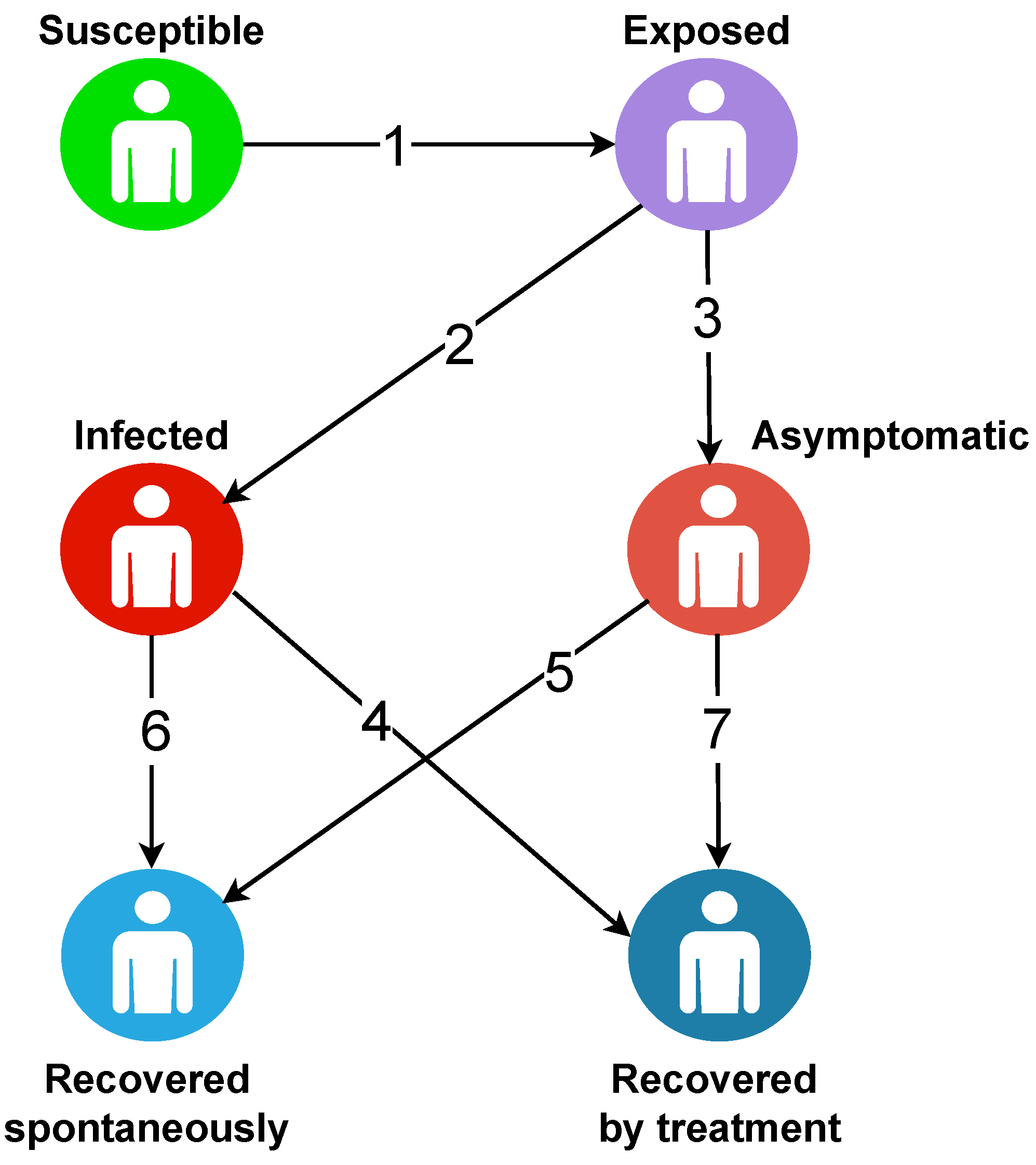
For this case study, we consider autonomous agents that represent the whole population with different statuses. S: Susceptible individuals, E: Latent or Exposed individuals, I: Infected individuals, A: Asymptomatic individuals, $R_1$: Recovered individuals, and $R_2$: Recovered spontaneously individuals. Figure 2 presents the transfer diagram of the multi-agent model.

With:

• Exposition.
• Visible infection.
• Hidden infection.
• Recovered of visible infection by treatment.
• Recovered of hidden infection without treatment.
• Recovered of visible infection without treatment.
• Recovered of hidden infection by treatment.

There is a strong case for addressing the different links that may exist between different agents. In the ABM, agents are not static either. They can undergo changes of state by contact or by the impulse of certain parameters. Further, this is why in this model, we have provided particular algorithms for each agent guiding the passage from one state to another.

Description of the Model Using ODD

To avoid any problems with the model results, we used the ODD (The Overview, Design concepts, and Details) protocol as a consistent, logical, and readable account of the ABM structures and dynamics [22].

• Overview
  • Objective: the interest of the model was to predict over a long period of time the incidental effects (evolution, treatment, management, brief scientific data) of the COVID-19 pandemic, and to understand the impact of the contact links between individuals in a precise contamination radius (environmental configuration) of the population.
  • Entities, state variables, and scales:

    -

    Agent or Individual: in the model we consider only one type of agent. Each agent has state variables and characteristics.

    -

    Environment: For a better-mixed population structural representation, we started from an environment in the form of a 50 × 50 mesh. An environment in which agents move randomly from one cell to another. Figure 3 shows this environment:

  • Process overview and scheduling: The model presents a process in discrete time steps.
    At the beginning of the simulation, all individual agents in the model are in any state (susceptible, exposed, infectious, asymptomatic, recovered, or recovered spontaneously). Each agent can move from one state to another according to a probability. Figure 4 displays the output of the model simulation at a given time t.
• Design Concepts
  • Basic principle: it is a propagation of the disease following a compartmental model containing six groups of individuals (susceptible, exposed, infected, asymptomatic, spontaneously recovered, and recovered with treatment).
    The idea here is that, initially, a susceptible individual comes into contact with an infectious individual. This contact gives the agent the opportunity to become either exposed or directly infected or asymptomatic. As a result, a newly exposed individual could also become either infected or asymptomatic. In the process, the infected or asymptomatic individual may either recover or succumb to the disease. There is also a prediction of natural death, which is an irrefutable factor.
  • Emerging: The emergence of the system is justified in the evolution of COVID-19 infection in the population. In fact, this emergence actually depends on several evolutionary factors that come into play: the type of agents that are initially infectious, other agents that come into contact with them along a contamination radius, the duration of contact but also the frequency of contact. However, there are some factors that surely have an impact on the readjustment of data.
  • Adaptation: Algorithms are designed to make agents able to reproduce different behaviors they observe in the environment. For example, in the mixed population structure, if an agent is already recovered, they will adapt their behavior by avoiding contact with infectious agents.
  • Detection: As infectious agents move through the environment, they can detect susceptible agents and recovered ones. Once recovered agents detect infectious agents, they avoid contact with them.
  • Interaction: In this model, we assume that agents in the same radius defined in the code interact with each other and with their environment. For example, if a patient agent is in the same radius as an infectious agent, it is possible for the patient agent to be contaminated.
  • Stochasticity: In a model, agents’ movements are random. With their specific states, agents’ movements are stochastic. Likewise, the choice of destinations for all agents is random. Stochasticity is also observed in COVID-19 contamination. If a susceptible agent comes into contact with an infectious agent, there is a certain likelihood that determines whether they are exposed, asymptomatic, or directly infectious. Additionally, the length of time an agent remains in a state (susceptible, exposed, infectious, asymptomatic, spontaneously recovered, or recovered after treatment) is chosen at random. So, in short, we are talking about a random pathway.
  • Observation: Data are collected at each model run on individual agents according to their states (susceptible, exposed, infectious, asymptomatic, recovered with treatment, or spontaneously).
• Details
  • Initialization: For the mixed population structure, agents are randomly placed in cells. At the start of the simulation, the environment contains only a given number of susceptible agents and a few infectious agents (chosen by the user).
  • Sub-models:

    -

    Timer: this sub-model manages the time in the system.

    -

    Death: death is considered here under both aspects, either natural or by disease also containing a drug failure. Infectious agents lose their lives with a certain probability.

    -

    Update of global variables: all global variables are updated at the end of each time step. At the same time, the number and percentage of susceptible, exposed, infected, asymptomatic, and recovered (spontaneously and after treatment) agents are all calculated.

6. Numerical Simulations and Results

6.1. EBM: Equation-Based Model

This first simulation was performed essentially on the various parameters proposed in [7,21]. We draw information from their setting before presenting the readjustment that we propose for a good study and a good follow-up.

6.2. EBM: Parameters Used

Parameters used were taken from the literature. Table 3 below presents these parameters, their meaning, and values.

6.2.1. EBM: Overview of the Results

• First scenario: Global dynamics
  In this first experiment, we present the global dynamics of the disease as a function of the basic reproduction number (${\mathcal{R}}_0$). With the baseline parameters presented in Table 3 above, we have a value ${\mathcal{R}}_0=3.2004$ that is close to the ${\mathcal{R}}_0$ average value obtained in [23] based on COVID-19 data from China in early 2020.
• Second scenario: Variation of the number of infected people as a function of ${\mathcal{R}}_0$.
  We can also see the progression curve of the disease as a function of the basic reproductions number (${\mathcal{R}}_0$), to see its impact on the dynamics of the epidemic.

• Third scenario: Variation of the number of infected I as a function of the recruitment rate ($\mathrm{\Lambda }$).
  This simulation scenario of the pandemic spread is formulated on the basis of the recruitment profile. Considering the recruitment of more and more susceptible individuals and based on the sensitivity value of the recruitment rate parameter with respect to ${\mathcal{R}}_0$ (see Table 2), it appears that this rate has a considerable impact on the spread of the disease.

6.2.2. EBM: Remarks

The mathematical model based on differential equations being completely deterministic, the simulation confirms the logic of the ${\mathcal{R}}_0$, which is for epidemiology and singularly for the EBM as a relevant indicator. Considering Figure 5, we can clearly see that ${\mathcal{R}}_0$ has an impact on the general dynamics of the disease. With the value of ${\mathcal{R}}_0=3.2004$, we find that the disease persists in the population over time. This is because one person infected with the SARS-CoV-2 coronavirus infects an average of $3.2$ new individuals. As the pandemic depends on parameter values that model it, we noticed a fast growth of the contamination curve as a function of some parameters, such as $\mathrm{\Lambda }$ and $\beta$, which are involved in the calculation of ${\mathcal{R}}_0$. This is confirmed in Table 2 which shows the high sensitivity value for these 2 parameters compared to the others. As shown in Figure 6, the larger the value of ${\mathcal{R}}_0$, the larger the number of infected people. This proves that the value of ${\mathcal{R}}_0$ has a considerable impact on the dynamics of the disease. Figure 7 shows the progression of infected individuals according to different values of the recruitment rate ($\mathrm{\Lambda }$).

6.3. ABM: Agent-Based Model

6.3.1. ABM: Parameters Used

Parameters used were taken from the literature.

Table 4. Parameters used for the agent-based model.

Parameters	Meaning	Values	References
$\mathrm{\Lambda }$	Recruitment rate	0.304	[7]
$\beta$	Contact rate	0.41	[24]
$\sigma$	Transmission rate to E	0.377	[7]
${ϵ}_1$	RPT rate of I	0.025	[7]
${ϵ}_2$	RWT rate of I	0.09497	[21]
${\lambda }_1$	RPT rate of A	0.04990	[21]
${\lambda }_2$	RWT rate of A	0.083	[21]
$\mu$	Mortality rate by disease	0.03890	[25]
$\delta$	Natural mortality rate	0.0192	[7]

below presents these parameters, their meaning, and values.

6.3.2. ABM: Overview of Results

• Scenario 1: Observation of the randomness of the approach.
  We observe the randomness of this approach while trying to present different simulations while keeping the same information, and from there we can clearly see that contrary to the EBM model, several simulations starting from identical INPUTS can produce quite different results. Thus, starting from the initial situation of 204 individuals including 2 infected and 2 asymptomatic, we present below some executions of the model at time $t=32$, in a radius of 5, with green: susceptible, yellow: exposed, red: infected, pink: asymptomatic, blue: RPT, white: RWT.
• Scenario 2: Observation of the results according to the radius.
  In this model, which is based on a stochastic modeling paradigm, there is a very important parameter to take into account: the “radius”. Indeed, this parameter clearly explains the decision of social distancing promulgated by the responsible authorities. Let us now analyze the traffic pattern in relation to the different radius values used.

6.3.3. ABM: Remarks

Based on the results obtained, we note that the disease dynamics follow a completely stochastic behavior, where at each execution of the performed simulation, there are different observations such as Figure 8a that represents the initial situation, Figure 8b gives us 0.49% of exposed, 4.9% of infected, 2.45% of asymptomatic, 1.47% of RPT, 0.49% of RWT, Figure 8c gives us 1.47% of exposed, 3.9% of infected, 2.9% of asymptomatic, 0.49% of RPT, 0% of RWT, and Figure 8d gives us 0.98% of exposed, 1.47% of infected, 1.96% of asymptomatic, 0.98% of RPT, 0% of RWT. The aspect of things verifies the random character of the model. We have also observed one of the very important parameters of the agent modeling, which is the radius, because it is an ABM modeling that establishes a detailed study on the inter-individual contact and we clearly see that although enjoying a random behavior, the radius can impact the pace of the propagation. Therefore, we have analyzed at the same time $t=23$, the dynamics of the mixed population through different values of radius. We clearly notice with Figure 9, Figure 10 and Figure 11 that when the radius of contagion is small, the disease takes a long time to settle in the population.

6.4. General Discussions

Thanks to the simulation, on the side of the EBM approach, we could observe the disease on many deterministic angles. It is precisely in this perspective that we were able to realize that the dynamics of the disease depends essentially on the parameters or different rates accompanying the models, such as $\lambda$, $\beta$, to mention only these. We also note that this way of doing things allows us to confirm the disease momentum with respect to the indicator parameter ${\mathcal{R}}_0$, where we can obviously see that the epidemic grows with ${\mathcal{R}}_0$.

With the ABM approach, we observed more clearly the evolution of the disease with regard to inter-individual relationships with a particular focus on a relevant parameter that we call the radius, relying more on the stochastic dynamics. The simulation obviously confirms the fact that equation-based models are fast (run time) compared to agent-based models. We can also observe in Figure 12, by varying the number of susceptible individuals, some distinctive aspects between the two approaches can be seen. The curves of the equation-based model are smooth, contrary to those of the agent-based models that have a certain randomness introduced by the stochastic aspect of the agents.

Figure 12a,c,e represent simulations of the equation-based model. The model is deterministic. Figure 12b,d,f represent simulations from ABM. This model is stochastic.

Table 5. Time cycle comparison table.

Number of Susceptible People	ABM	EBM
100	283 cycles	25 cycles
200	340 cycles	28 cycles
500	420 cycles	30 cycles
1000	500 cycles	35 cycles
5000	600 cycles	38 cycles
Average CPU load	50.4%	35.4%
Average Mem. Capacity	715.5 Mo	650.6 Mo

presents experiment results carried out using a computer with the following characteristics: ACER Aspire E5-571, Intel(R) core i3, with 4 × 1.7 Ghz CPU, and a 4096 MB RAM.

7. Concluding Remarks

In this paper, we have noted a major problem shaking our society: “the context of precarious life impacted by the COVID-19 pandemic”. To address this problem, we explored two approaches: equation-based modeling and agent-based modeling on the spread of diseases, especially during the COVID-19 pandemic. Then, we proposed a compartmental model of SEIAR-type describing the transfer diagram of COVID-19 dynamics. Based on the results obtained, it seems, on the one hand, that EBM is synthetic, formalized, homogeneous, and faster. Moreover, modeling with equations tends to describe reality at the macroscopic level. The model is far from the biological reality of the studied phenomenon. On the other hand, ABM is modular, incremental, heterogeneous, and close to the biological reality of the studied phenomenon since the description is made at the individual level. A few drawbacks were raised with ABM: the model is not formalized and requires many parameters, high runtime, and high memory capacity, as shown in Table 5.

Both approaches can be used to model the problem studied in this paper. However, it would be advisable to combine them to understand the reality, since none of them seem to outrank the other on the desirable criteria for a modeling approach.

8. Future Works

Indeed, the greatest challenge in an epidemiological study is to link the macroscopic aspect to the microscopic one. The latter can only be achieved by adopting a hybrid approach. Thus, we confirm that it would be much more relevant to couple the two models under a hybrid paradigm following the example of other scientists, such as [8], in order to take advantage of the two models. The whole starts from a compartmental model SEIAQR, with ideas of inserting one compartment such as the “QUARANTINE” type.

References

1. Jasper, F.W.C.; Kok, K.-H.; Zhu, Z.; Chu, H.; To, K.K.-W.; Yuan, S.; Yuen, K.-Y. Genomic characterization of the 2019 novel human-pathogenic coronavirus isolated from patients with acute respiratory disease in Wuhan, Hubei, China. Emerg. Micr. Infect. 2020, 9, 221–236. [Google Scholar]
2. Bahl, P.; Doolan, C.; de Silva, C.; Chughtai, A.A.; Bourouiba, L.; MacIntyre, C.R. Airborne or droplet precautions for health workers treating COVID-19? J. Infect. Dis. 2020, 225, 1561–1568. [Google Scholar] [CrossRef] [PubMed] [Green Version]
3. Booth, T.F.; Kournikakis, B.; Bastien, N.; Ho, J.; Kobasa, D.; Stadnyk, L.; Li, Y.; Spence, M.; Paton, S.; Henry, B.; et al. Detection of airborne severe acute respiratory syndrome (SARS) coronavirus and environmental contamination in SARS outbreak units. J. Infect. Dis. 2005, 191, 1472–1477. [Google Scholar] [CrossRef] [PubMed]
4. Zuo, W.; Zhao, X.; Chen, Y.-G. Molecular Biology of SARS-Coronavirus. In Chapter 5: SARS Coronavirus and Lung Fibrosis; Sunil, K.L., Ed.; Springer: Berlin/Heidelberg, Germany, 2010; pp. 247–258. [Google Scholar]
5. Kasereka, S. Modélisation Hybride de la Propagation des éPidemies et Estimation des Paramètres. Master’s Thesis, IFI, VNU, Hanoi, Vietnam, 2013. [Google Scholar]
6. Kasereka, S.; Le Strat, Y.; Léon, L. Estimation of infection force of hepatitis c virus among drug users in France. In Recent Advances in Nonlinear Dynamics and Synchronization; Springer: Berlin/Heidelberg, Germany, 2018; pp. 319–344. [Google Scholar]
7. Ndondo, A.M.; Kasereka, S.K.; Bisuta, S.F.; Kyamakya, K.; Doungmo, E.F.G.; Ngoie, R.-B.M. Analysis, modeling and optimal control of COVID-19 outbreak with three forms of infection in Democratic Republic of the Congo. Results Phys. 2021, 24, 104096. [Google Scholar] [CrossRef] [PubMed]
8. Kasereka, S.K. Towards hybrid stochastic modeling and simulation of complex systems in multi-scale environments with case studies on the spread of tuberculosis in Democratic Republic of the Congo. Ph.D. Thesis, University of South Africa, Pretoria, South Africa, 2020. [Google Scholar]
9. Bozkurt, F.; Yousef, A.; Abdeljawad, T. Analysis of the outbreak of the novel coronavirus COVID-19 dynamic model with control mechanisms. Results Phys. 2020, 19, 103586. [Google Scholar] [CrossRef] [PubMed]
10. Zhang, Z.; Zeb, A.; Alzahrani, E. Dynamics of COVID-19 mathematical model with stochastic perturbation. Adv. Differ. Equ. 2020, 2020, 451. [Google Scholar] [CrossRef] [PubMed]
11. Kasaie, P.; Dowdy, D.W.; Kelton, W.D. An agent-based simulation of a tuberculosis epidemic: Understanding the timing of transmission. In Simulation: Making Decisions in a Complex World, Proceedings of the 2013 Winter Simulation Conference, Washington, DC, USA, 8–11 December 2013; IEEE Press: Piscataway, NJ, USA, 2013; pp. 2227–2238. [Google Scholar]
12. Kasereka, S.K.; Doungmo, E.-F.G.; Ho, V.T.; Kyamakya, K. A stochastic agent-based model and simulation for controlling the spread of tuberculosis in a mixed population structure. In Developments of Artificial Intelligence Technologies in Computation and Robotics, Proceedings of the 14th International FLINS Conference (FLINS 2020), Cologne, Germany, 18–21 August 2020; World Scientific: Singapore, 2020. [Google Scholar] [CrossRef]
13. Shannon, R.E. Simulation modeling and methodology. Acm SIGSIM Simul. Dig. 1977, 8, 33–38. [Google Scholar] [CrossRef] [Green Version]
14. Kasereka, S.; Kasoro, N.; Chokki, A.P. A hybrid model for modeling the spread of epidemics: Theory and simulation. In ISKO-Maghreb: Concepts and Tools for Knowledge Management (ISKO-Maghreb), Proceedings of the 2014 4th International Symposium, Algiers, Algeria, 9–10 November 2014; IEEE: Alger, Algerie, 2014; pp. 1–7. [Google Scholar] [CrossRef]
15. Tracy, M.; Cerdá, M.; Keyes, K.M. Agent based modeling in public health: Current applications and future directions. Annu. Rev. Public Health 2018, 39, 77–94. [Google Scholar] [CrossRef] [PubMed] [Green Version]
16. Anderson, R.M.; May, R.M. Helminth infections of humans: Mathematical models, population dynamics, and control. Adv. Parasitol. 1985, 24, 1–101. [Google Scholar] [PubMed]
17. Goufo, E.F.D.; Maritz, R.; Munganga, J. Some properties of the Kermack–McKendrick epidemic model with fractional derivative and nonlinear incidence. Adv. Differ. Equ. 2014, 2014, 278. [Google Scholar] [CrossRef] [Green Version]
18. Luke, D.A.; Stamatakis, K.A. Systems science methods in public health: Dynamics, networks, and agents. Annu. Rev. Public Health 2012, 33, 357–376. [Google Scholar] [CrossRef] [PubMed] [Green Version]
19. van den Driessche, P.; Watmough, J. Reproduction numbers and sub-threshold endemic equilibria for compartmental models of disease transmission. Math. Biosci. 2002, 180, 29–48. [Google Scholar] [CrossRef] [PubMed]
20. Kasereka Kabunga, S.; Doungmo Goufo, E.F.; Ho Tuong, V. Analysis and simulation of a mathematical model of tuberculosis transmission in Democratic Republic of the Congo. Adv. Differ. Equ. 2020, 2020, 642. [Google Scholar] [CrossRef]
21. Sinan, M.; Ali, A.; Shah, K.; Assiri, T.A.; Nofal, T.A. Stability analysis and optimal control of COVID-19 pandemic SEIQR fractional mathematical model with harmonic mean type incidence rate and treatment. Results Phys. 2021, 22, 103873. [Google Scholar] [CrossRef] [PubMed]
22. Grimm, V.; Berger, U.; Bastiansen, F.; Eliassen, S.; Ginot, V.; Giske, J.; Goss-Custard, J.; Gr, T.; Heinz, S.; Huse, G.; et al. A standard protocol for describing individual based and agent-based models. Ecol. Model. 2006, 198, 115126. [Google Scholar] [CrossRef]
23. Liu, Y.; Gayle, A.A.; Wilder-Smith, A.; Rocklöv, J. The reproductive number of COVID-19 is higher compared to SARS coronavirus. J. Travel Med. 2020, 27, taaa021. [Google Scholar] [CrossRef] [PubMed] [Green Version]
24. Bentout, S.; Chekroun, A.; Kuniya, T. Parameter estimation and prediction for coronavirus disease outbreak 2019 (COVID-19) in Algeria. Aims Public Health 2020, 7, 306–318. [Google Scholar] [CrossRef] [PubMed]
25. Götz, T.; Heidrich, P. Early stage COVID-19 disease dynamics in Germany: Models and parameter identification. J. Math. Ind. 2020, 10, 20. [Google Scholar] [CrossRef] [PubMed]
Figure 1. EBM—transfer diagram describing the COVID-19 dynamics in the population.
Mathematics 11 00253 g001
Figure 2. ABM—transfer diagram describing the COVID-19 dynamics in the population.
Mathematics 11 00253 g002
Figure 3. Global illustration of the agent environment with susceptible individuals: green; exposed individuals: yellow; infected individuals: red; asymptomatic individuals: pink; recovered individuals: blue; recovered spontaneously (without any treatment): white.
Mathematics 11 00253 g003
Figure 4. Random distribution of agents in a 50 × 50 grid environment for the discrete agent-based model. The colored dot represents individuals with their specific status (Susceptible: green; exposed: yellow; infected: red; asymptomatic: pink; recovered with treatment: blue; recovered without treatment: white).
Mathematics 11 00253 g004
Figure 5. General dynamics of the disease with R 0 = 3.2004 .
Mathematics 11 00253 g005
Figure 6. Illustration of the progression of the infected individuals according to the R 0 .
Mathematics 11 00253 g006
Figure 7. Progression of the infected individuals according to the parameter Λ . Blue color: Λ = 0.095 , blue color: Λ = 0.104 , and red color: Λ = 0.404 .
Mathematics 11 00253 g007
Figure 8. Simulations of the model according to parameter values from Table 4. With (a) the initial situation, (bd) display the disease evolution up to a given time t.
Mathematics 11 00253 g008
Figure 9. Dynamics of COVID-19 according to the radius of contamination equal to 1 m.
Mathematics 11 00253 g009
Figure 10. Dynamics of COVID-19 according to the radius of contamination equal to 2 m.
Mathematics 11 00253 g010
Figure 11. Dynamics of COVID-19 according to the radius of contamination equal to 5 m.
Mathematics 11 00253 g011
Figure 12. Comparative curves for the two models with: (a): the EBM for S = 100 ; (b): the ABM for S = 100 ; (c): the EBM for S = 500 ; (d): the ABM for S = 500 ; (e): the EBM for S = 1000 ; (f): the ABM for S = 1000 .
Mathematics 11 00253 g012