Newton-Based Extremum Seeking for Dynamic Systems Using Kalman Filtering: Application to Anaerobic Digestion Process Control

Abstract

In this paper, a new Newton-based extremum-seeking control for dynamic systems is proposed using Kalman filter for gradient and Hessian estimation as well as a stochastic perturbation signal with time-varying amplitude. The obtained Kalman filter based Newton extremum-seeking control (KFNESC) makes it possible to accelerate the convergence to the extremum and attenuate the steady-state oscillations. The convergence and oscillation attenuation properties of the closed-loop system with KFNESC are considered, and the proposed control is applied to a two-stages anaerobic digestion process in order to maximize the hydrogen production rate, which has better robustness and a slower steady-state oscillation with the comparison of Newton-based ESC and sliding mode ESC.

1. Introduction

In many practical control problems, it is necessary to optimize the system output when the mathematical model of the system is partially or completely unknown. Extremum-seeking control (ESC) is largely used to solve such problems. ESC is an adaptive optimization algorithm that needs only input and output data to keep the system in the optimal operating point in real time. Stability conditions for ESC of nonlinear systems [1] were obtained in 2000, and then various ESC algorithms were proposed: multi-input extremum seeking control [2], slope extremum seeking control [3] discrete time extremum seeking control [4], sliding mode extremum seeking control [5] and others. At the same time, ESC has been applied in many fields, such as ABS (Automative Brake Systems) [6], flight formation [7], biotechnological process control [8,9], etc.

An important problem in ESC design is to ensure sufficiently fast convergence of the system output to its optimal operating point. A number of techniques have been proposed to accelerate the ESC convergence speed. In 2003, the sliding mode extremum-seeking control was developed [10], which can make the system to converge to the extreme point at a speed set in advance. In 2010, the Newton-based extremum-seeking control was proposed [11] and then it was extended to higher-order systems [12] and multi-input systems [13,14]. To obtain a more accurate gradient estimate for the system output equilibrium map, the recursive least squares method was used [15]. The recursive least squares estimation method with forgetting factor was further utilized [16] in ESC. In recent years, Lie bracket method has been widely used [17,18] in extremum-seeking and conditions for ESC uniform asymptotic stability have been obtained. The non-local stability properties of ESC are considered in [19,20].

In ESC, a perturbation signal is superimposed to the estimated value of the system control parameter so that the system output converges oscillatorily to its extremal value. In the classical ESC, the perturbation signal is a periodic signal. The effects of periodic perturbation signals with different amplitudes and jitter shapes on the ECS performances are compared and analyzed [21] in terms of convergence speed, convergence range, and accuracy. In 2009, stochastic perturbations were applied [22] for extremum seeking and then stability conditions were obtained [23] for ESC using a stochastic perturbation signal. Later, stochastic perturbations were applied [24,25] to classical ESC and Newton-based ESC.

In the mentioned ESC algorithms, the amplitude of the perturbation signal remains constant when the system reaches the optimal operating point, which can provoke important oscillations and excessive wear of the system actuators. To reduce the perturbation signal amplitude in steady-state regime, Lyapunov-based extremum seeking control has been proposed [26]. Using Lyapunov function, it is detected when the steady-state period is reached, and then the amplitude of the perturbation signal is decreased exponentially. An extremum-seeking algorithm without steady-state oscillations has been proposed [27]. In this algorithm the amplitude of the periodic excitation signal changes based on the gradient information, so as to avoid steady-state oscillations. A similar approach has been used in [28]. The ESC algorithm [29] uses sinusoidal detection technology to automatically distinguish between steady-state and transient modes in the extremum seeking process and cuts off the periodic perturbation signal when the steady-state regime is reached.

In this paper, we propose a model-free Newton-based extremum seeking control for dynamic systems as well as a stochastic perturbation signal in which instead of a combination of linear filters, a Kalman filter (KF) is used to estimate the gradient and Hessian of the system output equilibrium map. The KF based estimator makes it possible to obtain more accurate gradient and Hessian estimates, which enables speeding up the convergence to the extremum [30,31]. To attenuate the steady-state oscillations, a stochastic perturbation signal with decreasing amplitude is used. This algorithm is more realistic for practical realization than those in [32], where an inverse optimal neural control of a two-stage AD is proposed to follow hydrogen and methane production desired trajectories.

The paper is organized as follows. The proposed KFNESC is described in Section 2 and its convergence and oscillation attenuation are considered are considered in Section 3. The application of KFNESC to a two-stage anaerobic digestion process is presented and discussed in Section 4. The concluding remarks are given in Section 5.

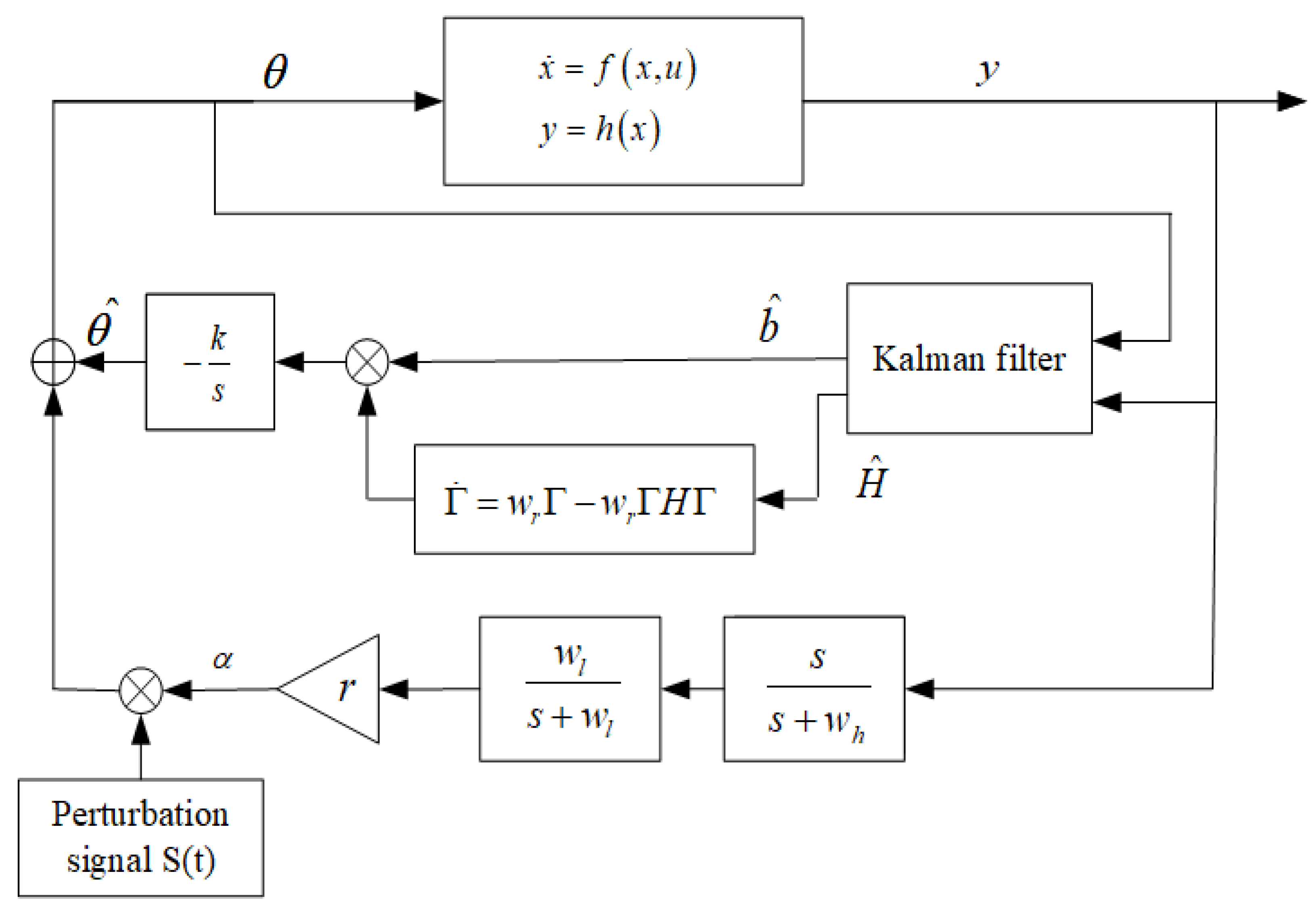
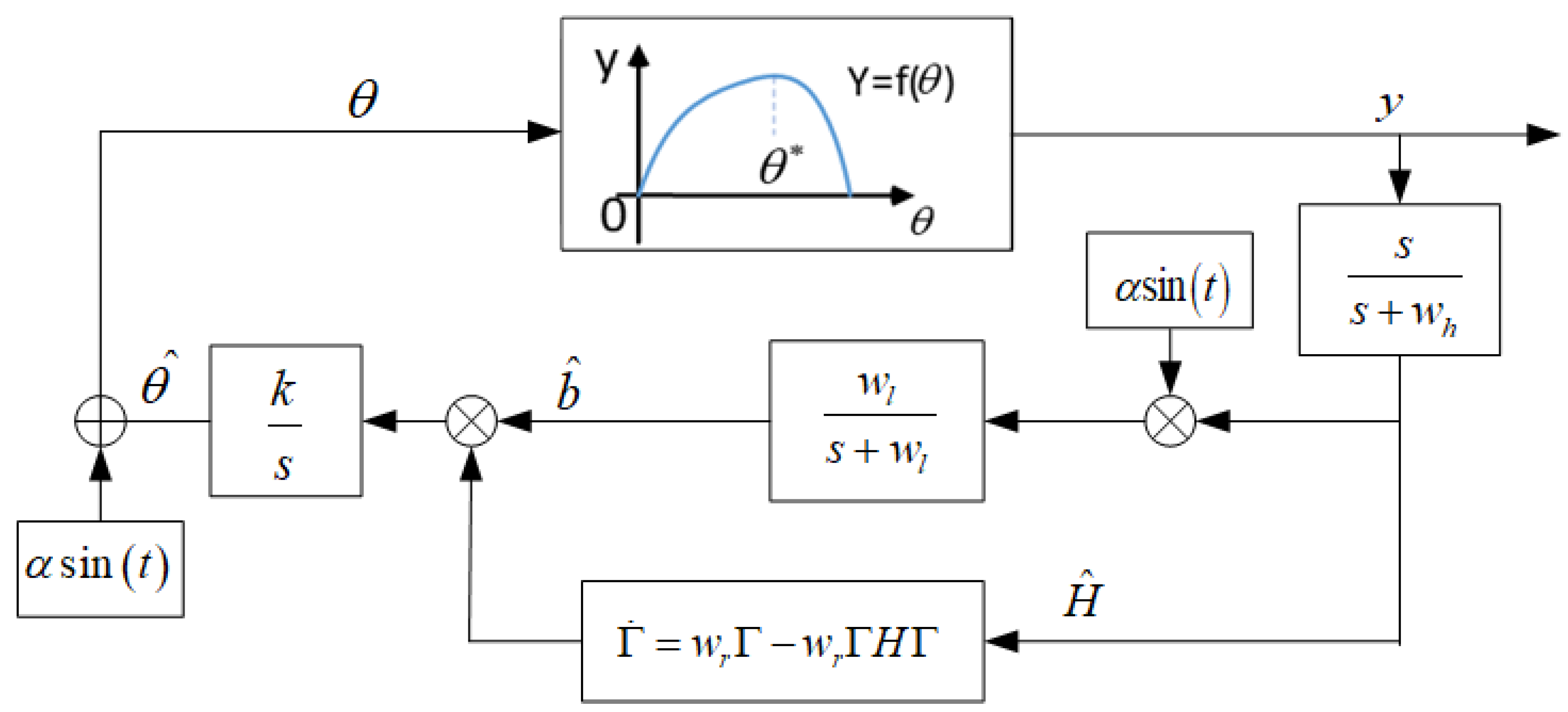
2. Extremum-Seeking Control for Dynamic Systems Using Newton Optimization and Kalman Filtering

Consider a single-input single-output nonlinear system

$$\{\begin{array}{l}\dot{x}=f(x,u)\\ y=h(x)\end{array}$$

(1)

where $x\in {\mathrm{R}}^n$ is the system state, $u\in \mathrm{R}$ is the input, $y\in \mathrm{R}$ is the output, $f:{\mathrm{R}}^n\times \mathrm{R}\to {\mathrm{R}}^n$ and $h:{\mathrm{R}}^n\to \mathrm{R}$ are smooth functions.

Let the smooth control law be similar to the following form $u=\alpha (u,\theta )$, which is parameterized by a scalar parameter $\theta \in \mathrm{R}$. Then, the closed-loop system has the unique equilibria parameterized by θ:

$$\dot{x}=f(x,\alpha (x,\theta ))$$

(2)

To optimize the system (2) using extremum-seeking control, it is assumed that:

• Assumption 1: There exists a smooth function $l:R\to R^n$ such that

  $$f(x,\alpha (x,\theta ))=0 \mathrm{if} \mathrm{and} \mathrm{only} \mathrm{if} x=l(\theta )$$

  (3)
• Assumption 2: For each $\theta$, the equilibrium $x=l(\theta )$ of system (2) is exponentially stable uniformly in $\theta$.
• Assumption 3: There exists ${\theta }^{*}\in R$ such that:

  $${\frac{\partial (h\circ l)}{\partial \theta }|}_{\theta ={\theta }^{*}}=0,\hspace{1em}{\frac{{\partial }^2(h\circ l)}{\partial {\theta }^2}|}_{\theta ={\theta }^{*}}=H<0$$

Thus, it is assumed that the output equilibrium map $y=h(l(\theta ))$ has a local maximum at $\theta \in {\theta }^{*}$.

The extremum-seeking control makes possible to maximize the steady-state value $y^{*}$ of the output without requiring the knowledge of either ${\theta }^{*}$ or the functions $y=h(x)$ and $x=l(\theta )$.

In this paper, a new extremum-seeking control for dynamic systems is proposed, combining the Newton algorithm [33] and the Kalman filter algorithm [34]. The advantage of Newton-based extremum-seeking over the gradient-based extremum-seeking is that the convergence speed is independent of the Hessian of output equilibrium map, but it is difficult to avoid system steady-state oscillations. The use of a Kalman filter (KF) to estimate the gradient and Hessian of the output equilibrium map makes it possible to speed up the convergence of the extremum-seeking algorithm. The steady-state oscillations are attenuated by using stochastic perturbation signal which amplitude tends to zero when the system output converges to its maximum. The schematic diagram of the proposed Kalman filter based Newton extremum-seeking control (KFNESC) is shown in Figure 1.

The system input $\theta$ is obtained by superimposing the perturbation signal $aS(t)$ to the estimate $\stackrel{⌢}{\theta }$ of $\theta$, which is produced by the Newton optimizer. In turn, the Kalman filter computes the real-time gradient and Hessian estimates $\widehat{b}$ and $\widehat{H}$ for the output equilibrium map $y=h(l(\theta ))$.

The estimate of the input $\widehat{\theta }$ is computed by the following Newton algorithm:

$$\frac{d\widehat{\theta }}{d{t}_{}}=-k\Gamma \widehat{b}$$

(4)

$$\frac{d\Gamma }{dt}=h\Gamma -h{\Gamma }^2\stackrel{⌢}{H}$$

(5)

until reaching the extremum point. Here, k, h > 0 are design parameters and $\Gamma$ is the estimate of the inverse of the Hessian matrix H of the output equilibrium map $y=h(l(\theta ))$. The Riccati Equation (5) has two equilibrium points: ${\Gamma }^{*}=0$ and ${\Gamma }^{*}={\stackrel{⌢}{H}}^{-1}$. Due to the fact $h>0$, only the equilibrium point ${\Gamma }^{*}={\stackrel{⌢}{H}}^{-1}$ is exponentially stable. Thus, $\Gamma$ can converge to the actual value of $H^{-1}$ if $\widehat{H}$ is a good estimate of the Hessian H. In addition, by tuning the value of parameter $h$, the convergence speed of the control algorithm can be adjusted to a certain extent.

To estimate the unknown gradient b and Hessian matrix H of $y=h(l(\theta ))$, both b and H are considered as discrete Kalman filter states: ${\left[\begin{array}{cc}{x}_1& x_2\end{array}\right]}^T={\left[\begin{array}{cc}b& H\end{array}\right]}^T$. The Kalman filter is implemented based on the following state and measurement equations:

$$\begin{array}{l}x(t_{k+1})=\left[\begin{array}{c}{x}_1(t_{k+1})\\ x_2(t_{k+1})\end{array}\right]=\left(\begin{array}{cc}1& 0\\ 0& 1\end{array}\right)x(t_k)+{\omega }_k\\ z(t_k)=\left[\begin{array}{c}\Delta y(t_k)\\ \Delta y(t_{k-n})\end{array}\right]=\underset{M_k}{\underbrace{\left[\begin{array}{cc}\Delta \theta (t_k)& \frac{1}{2}\Delta \theta {(t_k)}^2\\ \Delta \theta (t_{k-n})& \frac{1}{2}\Delta \theta {(t_{k-n})}^2\end{array}\right]}}x(t_k)+{\upsilon }_k\end{array}$$

(6)

where $\Delta y(t_k)=y(t_k)-y(t_{k-1}),$ $\Delta y(t_{k-n})=y(t_{k-n})-y(t_{k-n-1}),$ $\Delta \theta (t_k)=\theta (t_k)-\theta (t_{k-1}),$ $\Delta \theta (t_{k-n})=\theta (t_{k-n})-\theta (t_{k-n-1})$, and ${\omega }_k$, ${\upsilon }_k$ are independent normally distributed white noises with covariance matrices Q and R, respectively. The time-shifted input–output pair ($\Delta \theta (t_{k-n})$, $\Delta y(t_{k-n})$) is used to ensure the system observability. More details on the state estimation by KF in real time can be found [30].

The estimates $\widehat{b}$ and $\widehat{H}$ of $b$ and $H$ are calculated by the following Kalman filter algorithm [31]:

$$\begin{array}{l}{P}_k^{-}=P_{k-1}+Q\\ {\widehat{x}}_k={\widehat{x}}_{k-1}+P_k^{-}{M}_k^T{R}^{-1}(z_k-M_k{\widehat{x}}_k^{-})\\ P_k={(P_k^{-}+M_k^T{R}^{-1}{M}_k)}^{-1}\end{array}$$

(7)

where $x_k={\left[\begin{array}{cc}{x}_{1k}& x_{2k}\end{array}\right]}^T={\left[\begin{array}{cc}{b}_k& H_k\end{array}\right]}^T$, ${\widehat{x}}_{k-1}$ and ${\widehat{x}}_k$ are the state estimates at the k-th and k − 1 steps, $P_k^{-}$ and $P_k$ are the prior error covariance matrix and covariance matrix at step k, and $P_{k-1}$ is the covariance matrix at step k.

In order to attenuate the steady-state oscillations, the amplitude of the perturbation signal is adjusted so that it tends to zero when the system output y converges to its maximum. In this paper, we use perturbation signal $aS(t)$ with

$$a=r\frac{w_l}{s+w_l}(y-\zeta ),\hspace{1em}\zeta =\frac{s}{s+w_h}y$$

(8)

$$S\left(t\right)=\sin \left(\eta \left(t\right)\right),\hspace{1em}\eta \left(t\right)=w\pi \left(1+\sin W\left(t\right)\right)$$

(9)

Here, $w_l$ and $w_h$ are the frequencies of the corresponding low-pass or high-pass filters, $r>0$ is a constant gain for adjusting the convergence speed, $W(t)$ is the standard Brownian motion process, and $w$ is a positive constant.

Combined with Figure 1, the equation of closed-loop control system can be described as follows:

$$\begin{array}{l}\theta =\widehat{\theta }+aS(t)\\ \dot{\widehat{\theta }}=-k\Gamma \widehat{b}\\ \widehat{b},\widehat{H}=KF(\theta ,y)\hspace{0.17em}\hspace{0.17em}\hspace{0.17em}\\ \dot{\Gamma }=h\Gamma -h\Gamma \widehat{H}\Gamma \hspace{0.17em}\hspace{0.17em}\hspace{0.17em}\\ a=r\frac{w_l}{s+w_l}(y-\varsigma )\\ \dot{\varsigma }=-w_{{}^h}\varsigma +w_{h}y\end{array}$$

(10)

where $KF(\cdot )\hspace{0.17em}$ is the Kalman filtering algorithm. In order to simplify the system properties study, $S(t)$ is regarded as a constant 1, $\widehat{b}$ and $\widehat{H}$ computed by the Kalman filter are considered as actual values of $b$ and $H$ at the current moment.

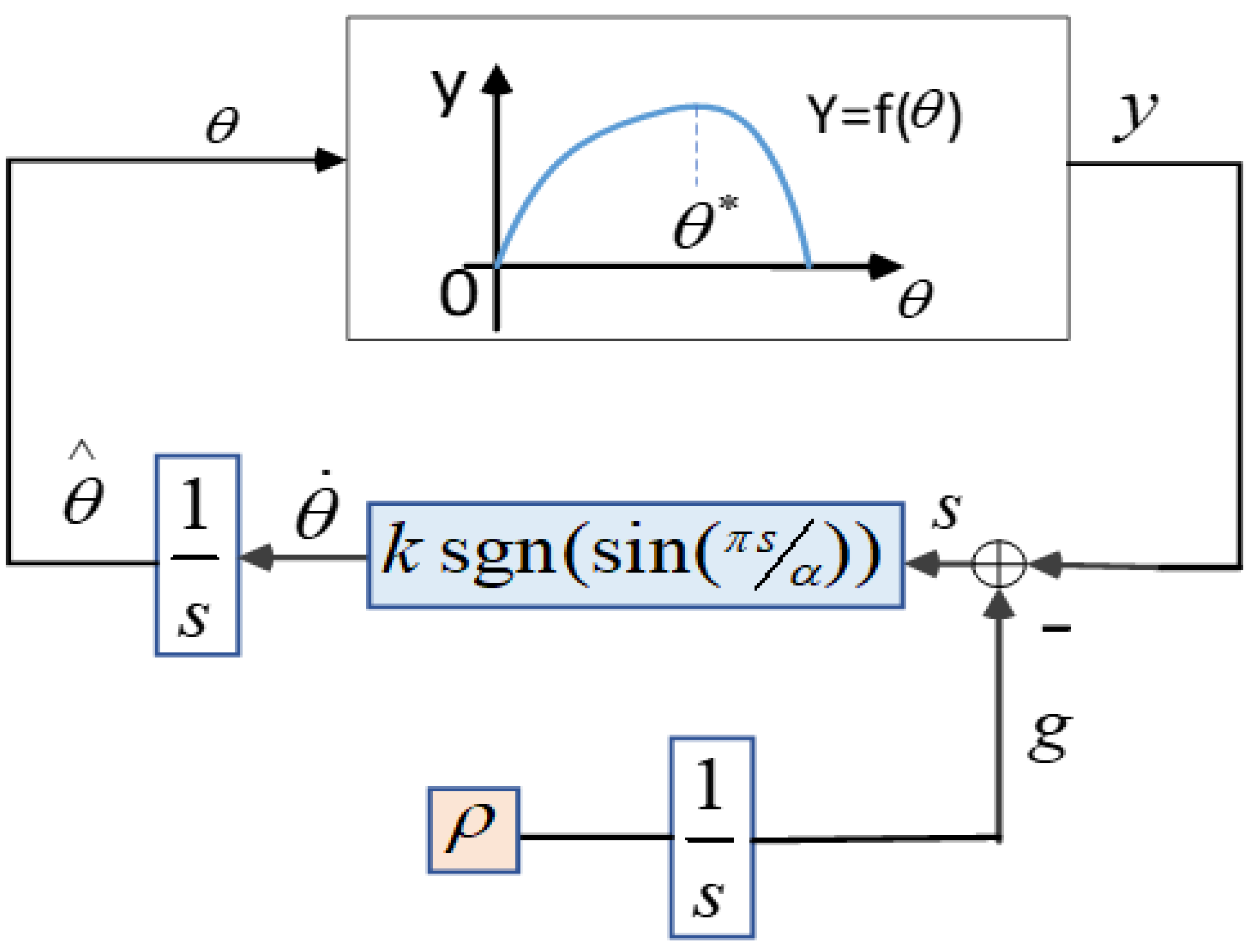
3. Convergence and Oscillation Attenuation Properties of the Closed-Loop System

In this section, the convergence and oscillation attenuation properties of the closed system with the proposed Kalman filter based Newton extremum-seeking control (KFNESC) are analyzed. The presented results on convergence and oscillation attenuation will be confirmed equally by the numerical simulations in the next section.

Firstly, the convergence of the Kalman filter based Newton extremum-seeking controller will be considered. To analyze the estimations $\widehat{b}$ and $\widehat{H}$, the static function between input and output $y=f\left(\theta \right)$ can be rewrite by Tayler expansion:

$$y=f\left(\theta \right)=f\left({\theta }^{*}\right)+\frac{f^{″}\left({\theta }^{*}\right)}{2}{\left(\theta -{\theta }^{*}\right)}^2$$

(11)

Define the error variables $\tilde{\theta }=\widehat{\theta }-{\theta }^{*}$, $\tilde{\Gamma }=\Gamma -H^{-1}$, $\tilde{\varsigma }=\varsigma -h\circ l({\theta }^{*})$, and the estimation of the gradient and Hessian in the dynamic systems can be written as:

$$\begin{array}{l}\widehat{b}=\frac{\partial f\left(\theta \right)}{\partial \theta }=\frac{\partial \left(f^{*}+\frac{f^{″}\left({\theta }^{*}\right)}{2}{\left(\tilde{\theta }+a\right)}^2\right)}{\partial \left({\theta }^{*}+\tilde{\theta }+a\right)}=f^{″}\left({\theta }^{*}\right)\left(\tilde{\theta }+a\right)=H^{*}\left(\tilde{\theta }+a\right)\\ \widehat{H}=\frac{{\partial }^{2}f\left(\theta \right)}{\partial {\theta }^2}=\frac{\partial b}{\partial \theta }=H^{*}\end{array}$$

(12)

with $H^{\ast }={\frac{{\partial }^2(h\circ l)}{\partial {\theta }^2}|}_{\theta ={\theta }^{*}}$.

Letting $x$ at its equilibrium value $x=l({\theta }^{*}+\tilde{\theta }+aS(t))$, the following error system on time scale $\tau =\delta t$ can be obtained [9,13,35]:

$$\frac{d}{d\tau }\left[\begin{array}{l}{\tilde{\theta }}_r\\ {\tilde{\Gamma }}_r\\ a_r\\ {\tilde{\varsigma }}_r\end{array}\right]=\delta \left[\begin{array}{l}k{H}^{*}({\tilde{\theta }}_r+a_r)({\tilde{\Gamma }}_r+H^{-1})\\ -h{\tilde{\Gamma }}_r{}^2{H}^{*}-h{\tilde{\Gamma }}_r\\ -w_l{a}_r+w_{l}r(h\circ l({\theta }^{*}+{\tilde{\theta }}_r+a_r)-h\circ l({\theta }^{*})-{\tilde{\varsigma }}_r)\\ -w_h{\tilde{\varsigma }}_r+w_h(h\circ l({\theta }^{*}+{\tilde{\theta }}_r+a_r))\end{array}\right]$$

(13)

for the fact that $H^{\ast }={\frac{{\partial }^2(h\circ l)}{\partial {\theta }^2}|}_{\theta ={\theta }^{*}}$.

With the averaging theorem $X_r=\frac{1}{T}{\displaystyle {\int }_t^{t+T}x\left(\tau \right)d\tau }$, the corresponding average error system can be deduced as follow:

$$\frac{d}{d\tau }\left[\begin{array}{l}{\tilde{\theta }}_r^a\\ {\tilde{\Gamma }}_r^a\\ a_r^a\\ {\tilde{\varsigma }}_r^a\end{array}\right]=\delta \left[\begin{array}{l}k{H}^{*}({\tilde{\theta }}_r^a+a_r^a)({\tilde{\Gamma }}_r^a+H^{-1})\\ -h{\tilde{\Gamma }}_r^{a2}{H}^{*}-h{\tilde{\Gamma }}_r^a\\ -w_l{a}_r-w_{l}r{\tilde{\varsigma }}_r^a+\frac{w_{l}r}{2\pi }{\displaystyle {\int }_0^{2\pi }v({\tilde{\theta }}_r^a+a_r^a)\mathrm{d}\omega }\\ -w_h{\tilde{\varsigma }}_r^a+\frac{w_h}{2\pi }{\displaystyle {\int }_0^{2\pi }v({\tilde{\theta }}_r^a+a_r^a)\mathrm{d}\omega }\end{array}\right]$$

(14)

Theorem 1.  

Consider system (14) under Assumption 3. The equilibrium point$[{\tilde{\theta }}_r^{a,e}\hspace{0.17em}{\tilde{\Gamma }}_r^{a,e}\hspace{0.17em}{a}_r^{a,e}\hspace{0.17em}{\tilde{\varsigma }}_r^{a,e}]$of (14) is stable.

Proof. 

The equilibrium point $[{\tilde{\theta }}_r^{a,e}\hspace{0.17em}{\tilde{\Gamma }}_r^{a,e}\hspace{0.17em}{a}_r^{a,e}\hspace{0.17em}{\tilde{\varsigma }}_r^{a,e}]$ satisfies the following equations:

$$\{\begin{array}{l}k{H}^{*}({\tilde{\theta }}_r^{a,e}+a_r^{a,e})({\tilde{\Gamma }}_r^{a,e}+H^{-1})=0\\ -h{\tilde{\Gamma }}_r^{a,e2}{H}^{*}-h{\tilde{\Gamma }}_r^{a,e}=0\\ \frac{w_{l}r}{2\pi }{\displaystyle {\int }_0^{2\pi }v({\tilde{\theta }}_r^{a,e}+a_r^{a,e}S(\omega ))S(\omega )\mathrm{d}\omega =}{w}_l{a}_r^{a,e}+w_{l}r{\tilde{\varsigma }}_r^{a,e}\\ \frac{w_h}{2\pi }{\displaystyle {\int }_0^{2\pi }v({\tilde{\theta }}_r^{a,e}+a_r^{a,e}S(\omega ))S(\omega )\mathrm{d}\omega }=w_h{\tilde{\varsigma }}_r^{a,e}\end{array}$$

(15)

At the equilibrium point $[{\tilde{\theta }}_r^{a,e}\hspace{0.17em}{\tilde{\Gamma }}_r^{a,e}\hspace{0.17em}{a}_r^{a,e}\hspace{0.17em}{\tilde{\varsigma }}_r^{a,e}]=[0\hspace{0.17em}0\hspace{0.17em}0\hspace{0.17em}0]$, the Jacobian matrix of the average system (14) can be calculated as:

$$J=\delta \left[\begin{array}{cccc}-k& 0& -k& 0\\ 0& -h& 0& 0\\ 0& 0& -w_l& 0\\ 0& 0& 0& -w_h\end{array}\right]$$

(16)

The matrix J is Hurwitz, which implies that the equilibrium of the average system is stable.

Secondly, let us analyze now the oscillation attenuation properties of the closed-loop system by perturbation signal. The amplitude of the perturbation signal $a$ affects both the steady-state and the dynamic performances of the system. The larger is the value of $a$, the better is the dynamic performance of the control algorithm, but the poorer is the steady-state performance.

By Tayler expansion and with Equation (11), one has the following output amplitude satisfying

$$\left|y-y^{*}\right|=\frac{1}{2}{\frac{{\partial }^2(h\circ l)}{\partial {\theta }^2}|}_{\theta ={\theta }^{*}}{(\tilde{\theta }+aS(t))}^2$$

(17)

$$a=\frac{r}{2}{\frac{{\partial }^2(h\circ l)}{\partial {\theta }^2}|}_{\theta ={\theta }^{*}}{\tilde{\theta }}^2$$

(18)

where $y^{\ast }=h(l({\theta }^{\ast }))$.

The error system being stable, $\tilde{\theta }$ will gradually converge to zero and the amplitude of the perturbation signal will approach zero with time. This means that the proposed extremum-seeking control algorithm makes attenuating steady-state oscillations possible.

Thus, the convergence and oscillation attenuation properties of the closed controlled system with the proposed KFNESC are successfully demonstrated. □

4. Application to Two-Stage Anaerobic Digestion Process Control

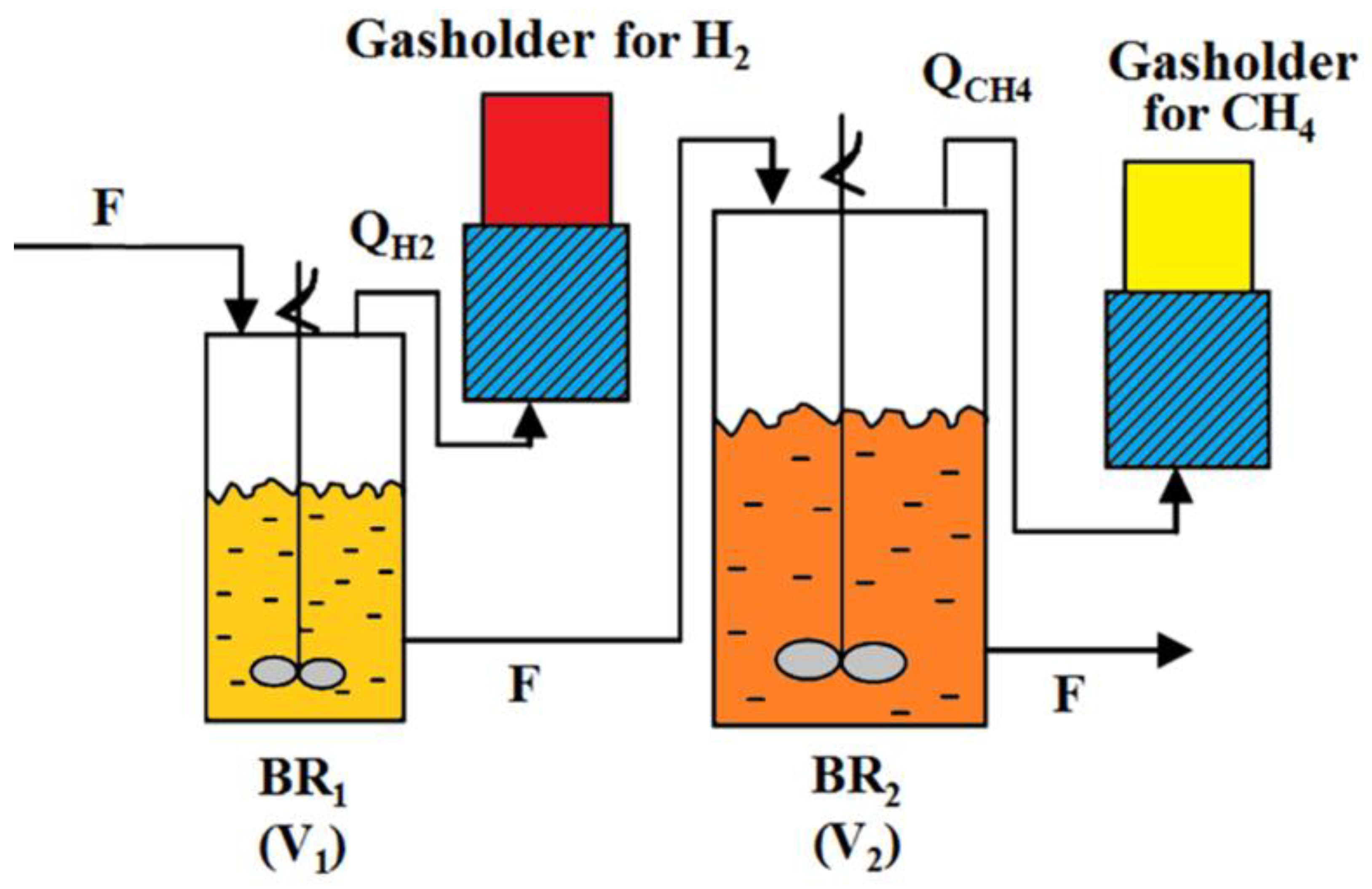
4.1. Process Description and Optimization Target

The anaerobic digestion (AD) process refers to a biochemical process in which anaerobic microorganisms convert biodegradable complex organic matter into simple compounds, such as methane, carbon dioxide, inorganic nutrients and humus in the absence of oxygen. Generally speaking, the AD process can be divided in four main phases of hydrolysis, acidogenesis, acetogenesis and methanogenesis. In the hydrolysis phase, undissolved complex organic compounds are hydrolyzed into small molecule compounds. In the acidogenesis stage, small molecule compounds are converted to volatile fatty acids (VFAs), hydrogen and carbon dioxide. In the acetogenesis phase, some VFAs (propionate and butyrate) are decomposed into acetate, hydrogen and carbon dioxide. In the methanogenesis phase, the acetoclastic methanogenic bacteria transform the acetate into methane and carbon dioxide.

A number of mathematical models for AD have been developed and investigated with a complete analysis for the existence and local stability of its steady states and conditions for maximal biogas production [36].

During the last 40 years, many different control methodologies for substrate feed control of the AD have been proposed, however full-scale biogas plants are mostly still operated without a closed-loop feed control and researchers have to design substrate feed control that does not rely on extensive online measurement equipment [37].

In recent years, an improved version of AD, known as two-stage AD, has become attractive among researchers for combined hydrogen and methane production from organic wastes [38,39]. The obtained mixed gas, known as bio-hydrogen can be used as fuel, and its thermal power is higher than petroleum derived fuel [40].

The two-stage AD system considered in this paper is a cascade of hydrogen reactor BR1 and methane reactor BR2 (see Figure 2) [41]. The bioreactors require the same inflows, and let F be the inflows in the first and second bioreactor. The reactor BR1 (with working volume V₁) performs the biochemical reactions in the hydrolysis and acidogenesis phases, while BR2 (with working volume V₂) performs acetogenic and methanogenic phases. The volatile fatty acids (VFAs)—acetate, propionate and butyrate, are produced in BR1 flow into BR2, where the propionate and butyrate will be further converted into acetate (acetogenic phase) and then into CH₄ and CO₂ (methanogenic phase).

The considered AD process has been simulated in MATLAB/Simulink using the following mathematical model [42]

$$\begin{array}{l}\frac{{\mathrm{dS}}_0}{\mathrm{dt}}=-D_1{\mathrm{S}}_0-\beta X_1{\mathrm{S}}_0+D_1{Y}_p{\mathrm{S}}_0^{\mathrm{in}}\\ \frac{{\mathrm{dS}}_1}{\mathrm{dt}}=-D_1{\mathrm{S}}_1+\beta X_1{\mathrm{S}}_0+\frac{{\mu }_1{X}_1}{Y_1}\\ \frac{{\mathrm{dX}}_1}{\mathrm{dt}}={\mu }_1{X}_1-D_1{X}_1\\ \frac{{\mathrm{dPr}}_1}{\mathrm{dt}}=\frac{{\mu }_1{X}_1}{Y_{\mathrm{Pr}1}}-D_1{\mathrm{Pr}}_1\\ \frac{{\mathrm{dBut}}_1}{\mathrm{dt}}=\frac{{\mu }_1{X}_1}{Y_{But1}}-D_{1}Bu{t}_1\\ \frac{{\mathrm{dAc}}_1}{\mathrm{dt}}=\frac{{\mu }_1{X}_1}{Y_{Ac1}}-D_{1}A{c}_1\\ Q_{H_2}=Y_{H_2}{\mu }_1{X}_1\end{array}\begin{array}{l}\frac{{\mathrm{dX}}_{\mathrm{Pr}}}{\mathrm{dt}}={\mu }_{\mathrm{Pr}}{X}_{\mathrm{Pr}}-D_2{X}_{\mathrm{Pr}}\\ \frac{{\mathrm{dPr}}_2}{\mathrm{dt}}=-\frac{{\mu }_{\mathrm{Pr}}{X}_{\mathrm{Pr}}}{Y_{ \mathrm{Pr}2}}+D_2({\mathrm{Pr}}_1-{\mathrm{Pr}}_2)\\ \frac{{\mathrm{dX}}_{\mathrm{But}}}{\mathrm{dt}}={\mu }_{But}{X}_{But}-D_2{X}_{But}\\ \frac{{\mathrm{dBut}}_2}{\mathrm{dt}}=-\frac{{\mu }_{But}{X}_{But}}{Y_{ But2}}+D_2(Bu{t}_1-Bu{t}_2)\\ \frac{{\mathrm{dX}}_{\mathrm{Ac}}}{\mathrm{dt}}={\mu }_{Ac}{X}_{Ac}-D_2{X}_{Ac}\\ \frac{{\mathrm{dAc}}_2}{\mathrm{dt}}=-\frac{{\mu }_{Ac}{X}_{Ac}}{Y_{ Ac2}}+\frac{{\mu }_{\mathrm{Pr}}{X}_{\mathrm{Pr}}}{Y_{ \mathrm{Pr}2}}+\frac{{\mu }_{But}{X}_{But}}{Y_{ But2}}\\ \hspace{0.17em}\hspace{0.17em}\hspace{0.17em}\hspace{0.17em}\hspace{0.17em}\hspace{0.17em}\hspace{0.17em}\hspace{0.17em}\hspace{0.17em}\hspace{0.17em}\hspace{0.17em}\hspace{0.17em}\hspace{0.17em}+D_2(A{c}_1-A{c}_2)\\ Q_{C{H}_4}=Y_{C{H}_4}{\mu }_{Ac}{X}_{Ac}\end{array}$$

(19)

where $S_0^{in}$, $S_0$ and $S_1$ are the concentrations of the inlet organic waste, macromolecular organics and soluble small molecule organics; $D_1$ and $D_2$ are the dilution rates of BR1 and BR2; X₁, X_Pr, X_But and X_AC denote, respectively, the acidogenic bacteria, propionic acid-degrading bacteria, butyric acid-degrading bacteria and methanogenic bacteria concentrations; Pr₂, But₂ and AC₂ are propionate, butyrate and acetate concentrations; and $Q_{H_2}$, $Q_{C{H}_4}$ represent the hydrogen and methane production rates. The model parameters are defined in

Table 1. Model parameters.

Parameter	Value	Parameter	Value
${\mu }_1{}_{\max }$	0.568	$Y_1$	0.08
${\mu }_{\mathrm{Pr}}{}_{\max }$	0.05	$Y_{\mathrm{Pr}1}$	4.2
${\mu }_{But}{}_{\max }$	0.05	$Y_{But1}$	2.1
${\mu }_{Ac}{}_{\max }$	0.025	$Y_{Ac1}$	1.1
$K_{s_1}$	3.914	$Y_{\mathrm{Pr}2}$	1.5
$K_{\mathrm{Pr}}$	0.22	$Y_{But2}$	1.5
$K_{But}$	0.22	$Y_{Ac2}$	0.5
$K_{Ac}$	0.8	$Y_{H_2}$	0.22
$\beta$	1	$Y_{C{H}_4}$	142
$Y_p$	1	-	-

[43].

Then, the objective of controlling anaerobic digestion processes is to obtain maximum quantity of biogases. In this article, the proposed extremum-seeking control is applied to the described AD system, considering the hydrogen production rate $Q_{H_2}$ as optimization target.

The AD process static characteristics $Q_{H_2}=Q_{H_2}(D_1)$ (Figure 3) show that for each inlet organics concentration ${\mathrm{S}}_0^{\mathrm{in}}$ there exists an optimal dilution rate $D_1$ where the maximal hydrogen production rate $Q_{H_2}^{*}$ is delivered. The maximum of $Q_{H_2}^{}$ depends on the concentration of organic waste $S_0^{in}$. The larger is the value of $S_0^{in}$, the larger is the maximal value of hydrogen production rate $Q_{H_2}^{}$.

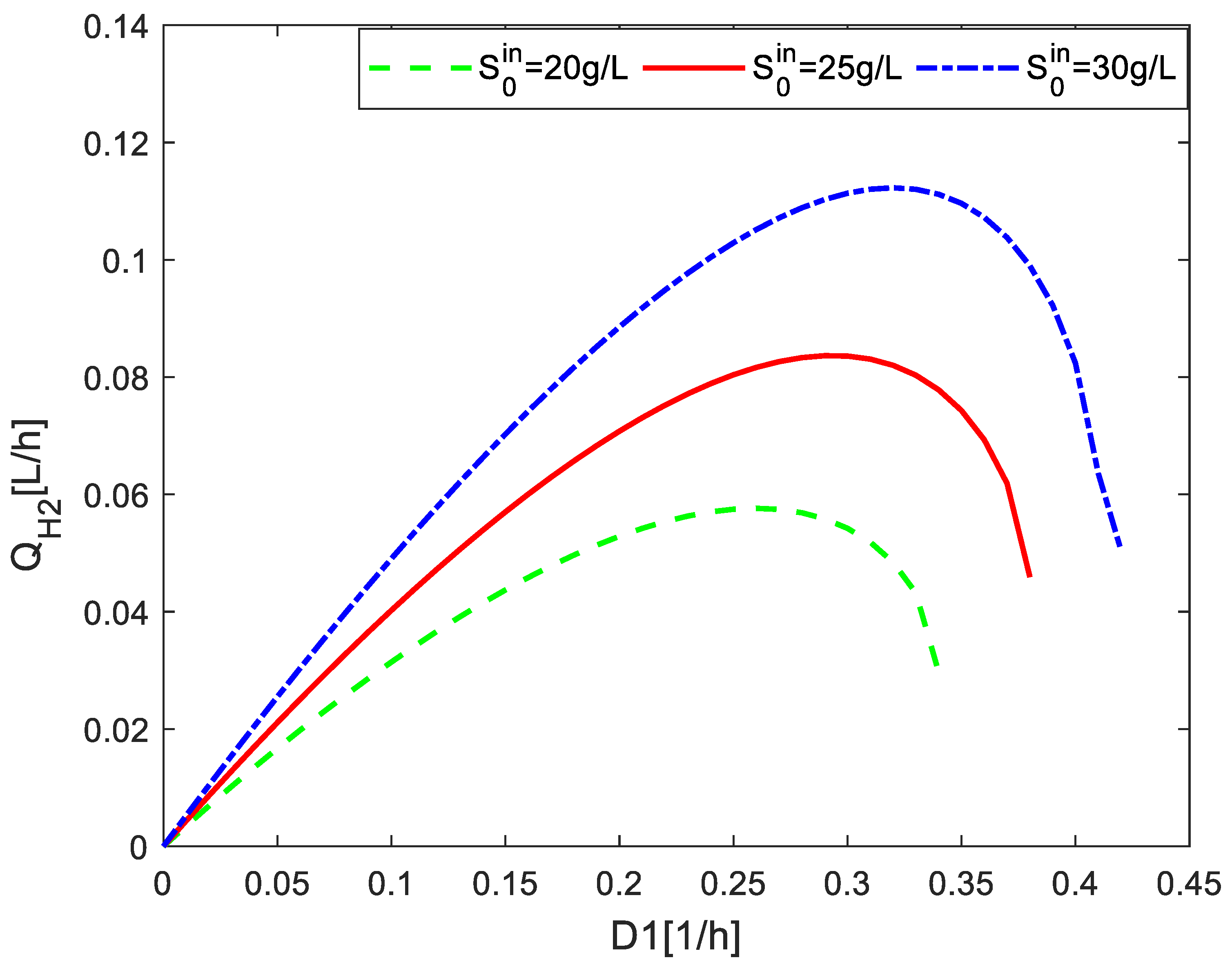
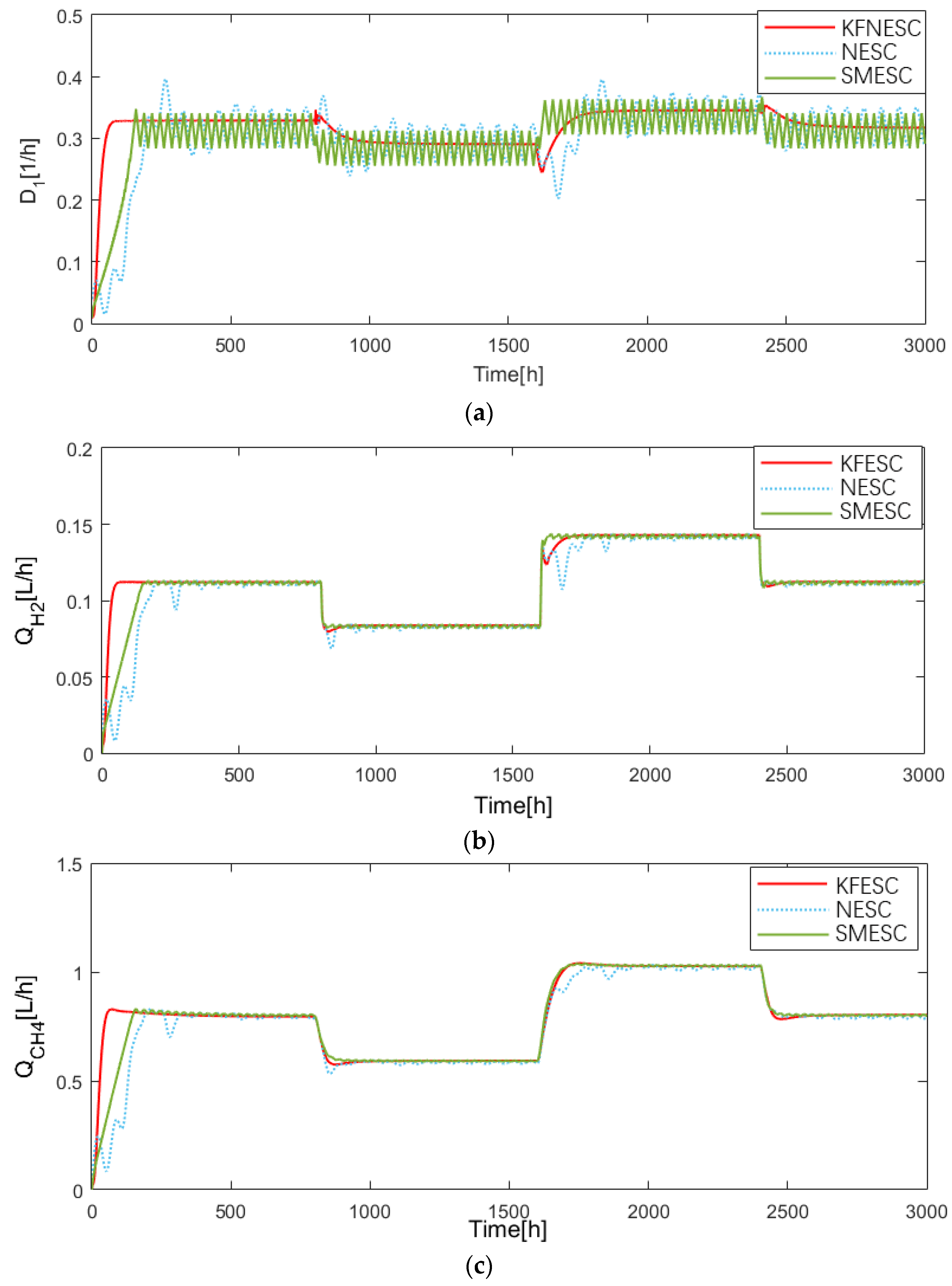
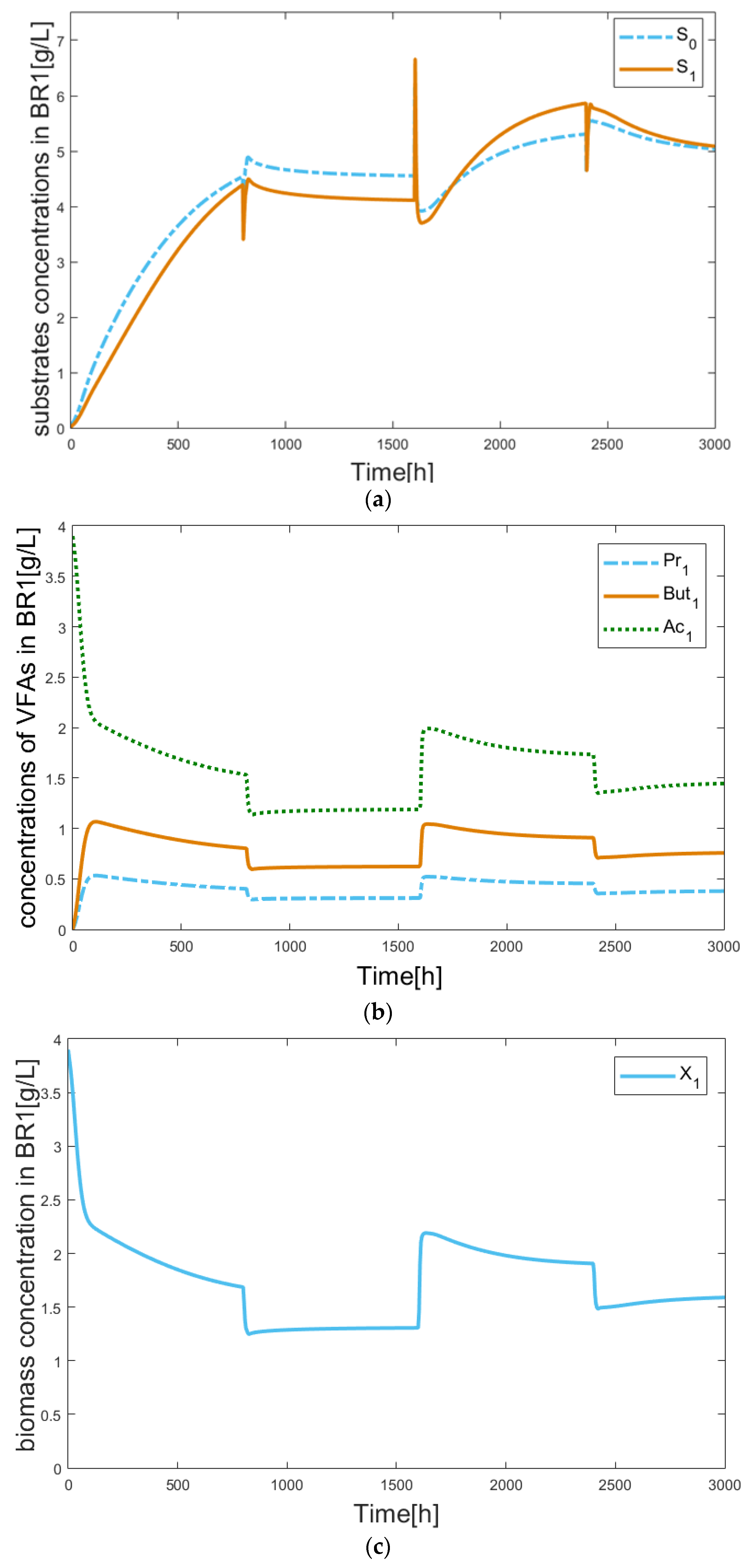
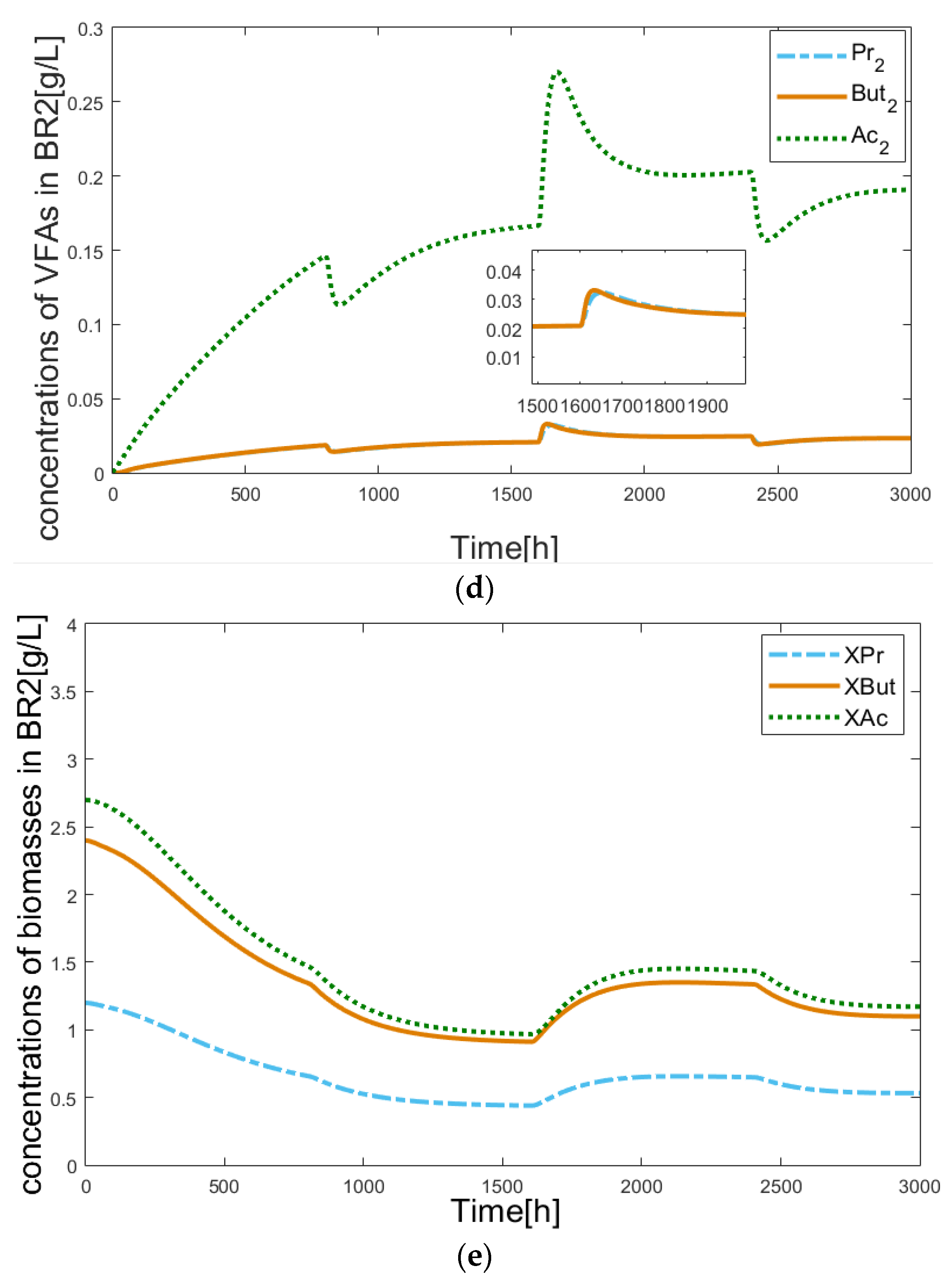
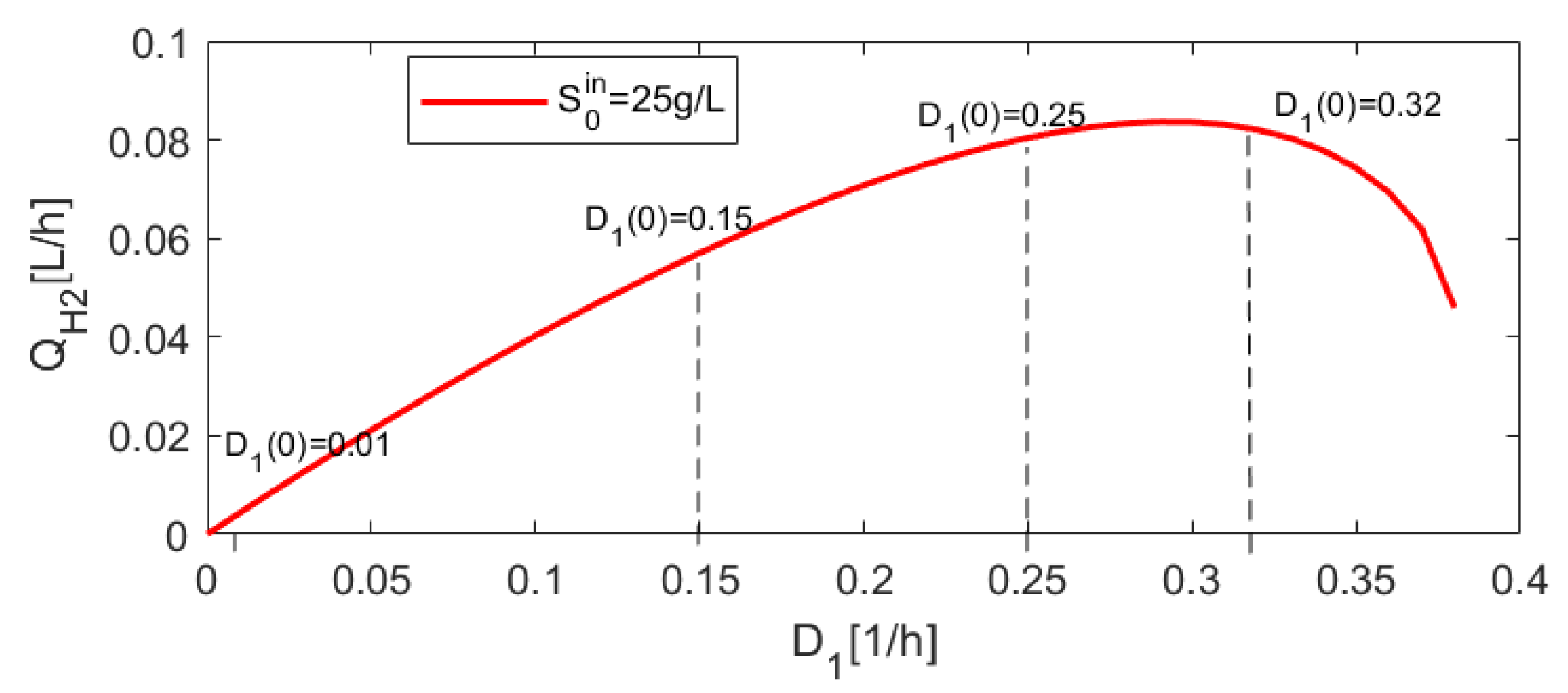
4.2. Numerical Simulations

In MATLAB/Simulink simulation experiments, we suppose that only the dilution rate $D_1$ and the hydrogen production rate $Q_{H_2}$ of the AD process are available for on-line measurement. A process optimization is realized by controlling the dilution rate $D_1$ in order to maximize the hydrogen production rate $Q_{H_2}$.

To demonstrate the performances of the proposed control, they are compared with the performances of the sliding mode ESC (SMESC) [10] and Newton-based ESC (NESC) [23]. The structure of the SMESC and NESC is shown in Figure 4 and Figure 5. KFNESC parameters are set as: $k$ = 0.0036, $r=1.6$, $w_l=0.02$, $w_h=0.08$, $w=0.1$ rad/s, $\Gamma (0)$ = −0.06. The perturbation signal frequency $w$ and the parameters $w_l$, $w_h$ of the linear filters in ESC and NESC are the same as those of KFNESC. The parameter k of ESC is set $k$ = 1. The SMESC design parameters are $k$ = 0.004 and $\beta$ = 0.0007. In turn, the NESC design parameters are $k$ = 5, $w_h=0.05,w_l=0.02,w_r=0.02$ and $\alpha$ = −0.03.

In the simulation experiment, the initial dilution rate $D_1(0)$ = 0.01 $h^{-1}$ and inlet organics concentration ${\mathrm{S}}_0^{\mathrm{in}}$ = 30 g/L. At 800 $h$ of the reaction, the inlet organics concentration step changed to 25 g/L. At 1600 $h$ of the reaction, the inlet organics concentration step changed to 35 g/L. At 2400 $h$ of the reaction, the inlet organics concentration step changed to 30 g/L. For the hydrogen production rate as optimization target, the obtained comparison results for SMESC, NESC and KFNESC are shown in Figure 6.

It can be seen that when the inlet organics concentration ${\mathrm{S}}_0^{\mathrm{in}}$ changes stepwise at 800 h, 1600 h and 2400 h, the proposed KFNESC ensures the shortest convergence time and smoothness of the dilution rate and gas production rate evolution. KFNESC also ensures dilution rate and gas production rate without chattering during steady state period.

The state variables trajectories of the AD process with KFNESC for ${\mathrm{S}}_0^{\mathrm{in}}$ stepwise changes and hydrogen production rate as optimization target are shown in Figure 7.

The trajectories of the operating point for different initial values of the dilution rate ($D_1(0)$ = 0.01, 0.15, 0.25, 0.32 $h^{-1}$) are given in Figure 8. It can be seen that regardless of whether the initial value of the dilution rate is on the left or on the right of the optimal value of $Q_{H_2}$, KFNESC can bring the AD system to the optimal operating point.

5. Conclusions

In this paper, a new Newton-based extremum-seeking control for dynamic systems is developed using a Kalman filter for gradient and Hessian estimation and a stochastic perturbation signal with decreasing amplitude. The Kalman filter makes it possible to obtain more accurate gradient and Hessian estimates for the output equilibrium map and to speed up the convergence to the optimal operating point of the controlled system. When the system output converges to the maximum value, the system has better robustness, and the amplitude of the disturbance signal approaches zero thereby attenuating the steady-state oscillation of the system.

The new extremum-seeking control is applied to a two-stage anaerobic digestion process in order to maximize the hydrogen production rate. The performances of the proposed control are compared by numerical simulations with the performances of the existing Newton-based extremum-seeking control and the sliding mode extremum-seeking control. The obtained simulation results demonstrate the better performances of the new extremum-seeking control in comparison with the existing extremum-seeking controls.

Future work will be realized in order to apply the proposed extremum-seeking control method to a real two-stage AD process and to generalize this method for multi input nonlinear systems.

References

1. Wang, H.H.; Krstic, M. Extremum seeking for limit cycle minimization. In Proceedings of the 39th IEEE Conference on Decision and Control, Sydney, NSW, Australia, 12–15 December 2000; Volume 3, pp. 2438–2442. [Google Scholar]
2. Ariyur, K.B.; Krstic, M. Analysis and design of multivariable extremum seeking. In Proceedings of the 2002 American Control Conference, Anchorage, AK, USA, 8–10 May 2002; Volume 4, pp. 2903–2908. [Google Scholar]
3. Ariyur, K.B.; Krstic, M. Slope seeking: A generalization of extremum seeking. Int. J. Adapt. Control. Signal Process. 2004, 18, 1–22. [Google Scholar] [CrossRef]
4. Guay, M.; Dochain, D. A time-varying extremum-seeking control approach. Automatica 2015, 51, 356–363. [Google Scholar] [CrossRef]
5. Ozgüner, U.; Fu, L. Variable structure extremum seeking control based on sliding mode gradient estimation for a class of nonlinear systems. In Proceedings of the 2009 American Control Conference, St. Louis, MO, USA, 10–12 June 2009; pp. 8–13. [Google Scholar]
6. Dincmen, E.T.; Acarman, B.G. Abs control algorithm via extremum seeking method with enhanced lateral stability. IFAC Proc. Vol. 2010, 43, 19–24. [Google Scholar] [CrossRef]
7. Binetti, P.; Ariyur, K.B.; Krstic, M.; Bernelli, F. Formation flight optimization using extremum seeking feedback. J. Guid. Control. Dyn. 2003, 26, 132–142. [Google Scholar] [CrossRef] [Green Version]
8. Atta, K.T.; Johansson, A.; Gustafsson, T. On-Line Optimization of Cone Crushers using Extremum-Seeking Control. In Proceedings of the IEEE International Conference on Control Technology and Applications, Hyderabad, India, 28–30 August 2013; pp. 1054–1060. [Google Scholar]
9. Simeonov, I.; Noykova, N.; Gyllenberg, M. Identification and extremum seeking control of the anaerobic digestion of organic wastes. Cybern. Inf. Technol. 2007, 7, 73–84. [Google Scholar]
10. Pan, Y.; Özgüner, Ü.; Acarman, T. Stability and performance improvement of extremum seeking control with sliding mode. Int. J. Control. 2003, 76, 968–985. [Google Scholar] [CrossRef]
11. Moase, W.H.; Manzie, C.; Brear, M.J. Newton-like extremum-seeking for the control of thermoacoustic instability. IEEE Trans. Autom. Control. 2010, 55, 2094–2105. [Google Scholar] [CrossRef]
12. Nešić, D.; Tan, Y.; Moase, W.H.; Manzie, C. A unifying approach to extremum seeking: Adaptive schemes based on estimation of derivatives. In Proceedings of the IEEE Conference on Decision and Control, Atlanta, GA, USA, 15–17 December 2010; pp. 4625–4630. [Google Scholar]
13. Ghaffari, A.; Krstić, M.; Nešić, D. Multivariable newton-based extremum seeking. Automatica 2012, 48, 1759–1767. [Google Scholar] [CrossRef]
14. Salsbury, T.I.; Drees, K.H.; House, J.M.; Perez, C. Newton-Based Extremum-Seeking Control System. U.S. Patent US20200348635A1, 5 November 2020. [Google Scholar]
15. Dewasme, L.; Srinivasan, B.; Perrier, M.; Vande Wouwer, A. Extremum-seeking algorithm design for fed-batch cultures of microorganisms with overflow metabolism. J. Process Control. 2011, 21, 1092–1104. [Google Scholar] [CrossRef]
16. Chioua, M.; Srinivasan, B.; Guay, M.; Perrier, M. Performance improvement of extremum seeking control using recursive least square estimation with forgetting factor. IFAC-PapersOnLine 2016, 49, 424–429. [Google Scholar] [CrossRef]
17. Dürr, H.B.; Krstić, M.; Scheinker, A.; Ebenbauer, C. Extremum seeking for dynamic maps using Lie brackets and singular perturbations. Automatica 2017, 83, 91–99. [Google Scholar] [CrossRef]
18. Dürr, H.B.; Stanković, M.S.; Ebenbauer, C.; Johansson, K.H. Lie bracket approximation of extremum seeking systems. Automatica 2013, 49, 1538–1552. [Google Scholar] [CrossRef] [Green Version]
19. Tan, Y.; Nešić, D.; Mareels, I.M.Y. On non-local stability properties of extremum seeking control. Automatica 2006, 42, 889–903. [Google Scholar] [CrossRef] [Green Version]
20. Moase, W.H.; Tan, Y.; Nešić, D.; Manzie, C. Non-local stability of a multi-variable extremum-seeking scheme. In Proceedings of the 2011 Australian Control Conference, Melbourne, Australia, 10–11 November 2011; pp. 38–43. [Google Scholar]
21. Tan, Y.; Nešić, D.; Mareels, I. On the choice of dither in extremum seeking systems: A case study. Automatica 2008, 44, 1446–1450. [Google Scholar] [CrossRef]
22. Manzie, C.; Krstic, M. Extremum seeking with stochastic perturbations. IEEE Trans. Autom. Control. 2009, 54, 580–585. [Google Scholar] [CrossRef]
23. Liu, S.-J.; Krstic, M. Newton-based stochastic extremum seeking. Automatica 2014, 50, 952–961. [Google Scholar] [CrossRef]
24. Liu, S.-J.; Krstic, M. Stochastic Averaging and Stochastic Extremum Seeking; Communications and Control Engineering; Springer: London, UK, 2012. [Google Scholar]
25. Yin, C.; Wu, S.; Zhou, S.; Cao, J.; Huang, X.; Cheng, Y. Design and stability analysis of multivariate extremum seeking with newton method. J. Frankl. Inst. 2018, 355, 1559–1578. [Google Scholar] [CrossRef]
26. Moura, S.J.; Chang, Y.A. Lyapunov-based switched extremum seeking for photovoltaic power maximization. Control. Eng. Pract. 2013, 21, 971–980. [Google Scholar] [CrossRef]
27. Wang, L.; Chen, S.; Ma, K. On stability and application of extremum seeking control without steady-state oscillation. Automatica 2016, 68, 18–26. [Google Scholar] [CrossRef]
28. Zhang, L.; Hu, Y. Multi-parameter extremum seeking algorithm with amplitude tuned adaptively. Huazhong Keji Daxue Xuebao (Ziran Kexue Ban)/J. Huazhong Univ. Sci. Technol. (Nat. Sci. Ed.) 2016, 44, 53–57. [Google Scholar]
29. Mu, B.; Li, Y.; Seem, J.E. Discrimination of steady state and transient state of dither extremum seeking control via sinusoidal detection. Mech. Syst. Signal Process. 2016, 76, 93–110. [Google Scholar] [CrossRef]
30. Hun, L.C.; Yeng, O.L.; Sze, L.T.; Chet, K.V. Kalman Filtering and Its Real-Time Applications. In Real-Time Systems; IntechOpen: London, UK, 2016. [Google Scholar]
31. Mandić, F.; Mišković, N. Tracking underwater target using extremum seeking. IFAC-PapersOnLine 2015, 48, 149–154. [Google Scholar] [CrossRef]
32. Gurubel, K.; Sanchez, E.; Coronado, A.; Zúñga, V.; Sulbaran, B. Optimal neural control of a two stage anaerobic digestion model for biofuels production. In Proceedings of the IEEE International Joint Conference on Neural Networks, Rio de Janeiro, Brazil, 8–13 July 2018; pp. 265–271. [Google Scholar]
33. Zaman, A.; Birk, W.; Atta, K.T.; Mortsell, M. Adaptive Decoupling of Multivariable Systems Using Extremum-Seeking Approach. In Proceedings of the 26th IEEE International Conference on Emerging Technologies and Factory Automation (ETFA), Vasteras, Sweden, 7–10 September 2021. [Google Scholar]
34. Gaida, D.; Wolf, C.; Bongards, M. Feed control of anaerobic digestion process for renewable energy production: A review. Renew. Sustain. Energy Rev. 2017, 68, 869–875. [Google Scholar] [CrossRef]
35. Yin, C.; Dadras, S.; Huang, X.; Chen, Y.Q.; Zhong, S. Optimizing energy consumption for lighting control system via multivariate extremum seeking control with diminishing dither signal. IEEE Trans. Autom. Sci. Eng. 2009, 16, 1848–1859. [Google Scholar] [CrossRef]
36. Speyer, J.L.; Chung, W.H. Stochastic Processes, Estimation, and Control; Society for Industrial and Applied Mathematics: Philadelphia, PA, USA, 2008. [Google Scholar]
37. Weedermann, M.; Wolkowicz, G.; Sasara, J. Optimal biogas production in a model for anaerobic digestion. Nonlinear Dyn. 2015, 81, 1097–1112. [Google Scholar] [CrossRef]
38. Sari, T.; Benyahia, B. The operating diagram for a two-step anaerobic digestion model. Nonlinear Dyn. 2021, 105, 2711–2737. [Google Scholar] [CrossRef]
39. Moreno, J.A.; Besançon, G. On multi-valued observers for a class of single-valued systems. Automatica 2021, 123, 109334. [Google Scholar] [CrossRef]
40. Chorukova, E.; Hubenov, V.; Gocheva, Y.; Simeonov, I. Two-Phase Anaerobic Digestion of Corn Steep Liquor in Pilot Scale Biogas Plant with Automatic Control System with Simultaneous Hydrogen and Methane Production. Appl. Sci. 2022, 12, 6274. [Google Scholar] [CrossRef]
41. Ruggeri, B.; Tommasi, T.; Sanfilippo, S. BioH2 & BioCH4 through Anaerobic Digestion (From Research to Full-Scale Applications); Springer: London, UK, 2015; 215p. [Google Scholar]
42. Krishnan, S.; Md Din, M.F.; Mat Taib, S.; Ee Ling, Y.; Puteh, H.; Mishra, P.; Nasrullah, M.; Sakinah, M.; Wahid, Z.A.; Rana, S.; et al. Process constraints in sustainable bio-hythane production from wastewater: Technical note. Bioresour. Technol. Rep. 2019, 5, 359–363. [Google Scholar] [CrossRef]
43. Chorukova, E.; Simeonov, I.; Kabaivanova, L. Volumes Ratio Optimization in a Cascade Anaerobic Digestion System Producing Hydrogen and Methane. Ecol. Chem. Eng. S 2021, 28, 183–200. [Google Scholar] [CrossRef]
Figure 1. Structure of the Kalman filter based Newton extremum-seeking control for dynamic systems.
Mathematics 11 00251 g001
Figure 2. AD process with production of hydrogen and methane.
Mathematics 11 00251 g002
Figure 3. Static characteristics D 1 Q H 2 for different S 0 i n .
Mathematics 11 00251 g003
Figure 4. The Structure of the Sliding mode extremum-seeking control for dynamic systems.
Mathematics 11 00251 g004
Figure 5. The Structure of the Newton-based extremum-seeking control for dynamic systems.
Mathematics 11 00251 g005
Figure 6. AD processes for different ESC and hydrogen production rate as optimization target. (a) Input: dilution rate, (b) Optimization target: hydrogen production rate, (c) Methane production rate.
Mathematics 11 00251 g006
Figure 7. State variables trajectories of the AD process with KFNESC for S 0 in stepwise changes and hydrogen production rate as optimization target. (a) Trajectories of substrates concentrations in BR1, (b) Trajectories of concentrations of VFAs in BR1, (c) Trajectory of biomass concentration in BR1, (d) Trajectories of concentrations of VFAs in BR2, (e) Trajectories of concentrations of biomasses in BR2.
Mathematics 11 00251 g007aMathematics 11 00251 g007b
Figure 8. Trajectories of the operating point in the plan D 1 Q H 2 for different initial values of the dilution rate under KFNESC.
Mathematics 11 00251 g008