5G Multi-Slices Bi-Level Resource Allocation by Reinforcement Learning

Abstract

As the centralized unit (CU)—distributed unit (DU) separation in the fifth generation mobile network (5G), the multi-slice and multi-scenario, can be better applied in wireless communication. The development of the 5G network to vertical industries makes its resource allocation also have an obvious hierarchical structure. In this paper, we propose a bi-level resource allocation model. The up-level objective in this model refers to the profit of the 5G operator through the base station allocating resources to slices. The lower-level objective in this model refers to the slices allocating the resource to its users fairly. The resource allocation problem is a complex optimization problem with mixed-discrete variables, so whether a resource allocation algorithm can quickly and accurately give the resource allocation scheme is the key to its practical application. According to the characteristics of the problem, we select the multi-agent twin delayed deep deterministic policy gradient (MATD3) to solve the upper slice resource allocation and the discrete and continuous twin delayed deep deterministic policy gradient (DCTD3) to solve the lower user resource allocation. It is crucial to accurately characterize the state, environment, and reward of reinforcement learning for solving practical problems. Thus, we provide an effective definition of the environment, state, action, and reward of MATD3 and DCTD3 for solving the bi-level resource allocation problem. We conduct some simulation experiments and compare it with the multi-agent deep deterministic policy gradient (MADDPG) algorithm and nested bi-level evolutionary algorithm (NBLEA). The experimental results show that the proposed algorithm can quickly provide a better resource allocation scheme.

1. Introduction

With the advent of the fifth generation mobile network (5G) era, the high bandwidth of 5G provides the basis for serving massive users, thus opening a new era of multi-scenario the Internet of Everything in the orthogonal frequency division multiple access (OFDMA) system. There are three major application scenarios of the 5G: (1) massive machine type communications (mMTC) [1]; (2) enhanced mobile broadband (eMBB) [2]; (3) ultra-reliable and low-latency communication (URLLC) [3]. The overall architecture of the 5G has undergone big and small changes. For example, the 5G base station integrates the original remote radio unit (RRU) and antenna into the active antenna unit (AAU) to replace the RRU of the 4G base station in the wireless access network, which reduces the loss of the feed line from antennas to the RRU in the previous architecture. In the 5G bearer network, the building baseband unit (BBU) can separate optionally into a centralized unit (CU) and a distributed unit (DU), and some non-real-time functions of the BBU are integrated into DU and then sink to the AAU. The remaining real-time functions are integrated into CU. Therefore, they can be selectively separated into different application scenarios [4]. This structure application with the following network function virtualization (NFV) application will be more extensive. In the core network, different from the serving gateway and the packet data network gateway [5] of the 4G network, the 5G completely separates the control plane (CP) from the user plane (UP). Its advantages are flexible service changes, convenient network expansion and upgrades, and the user plane can be removed from the “centralized” position. It can be deployed in the core network or sunk into the access network, meeting the requirements of low latency 5G networks and providing great convenience for the maintenance and expansion of the 5G core network. This flexible networking mode brings great new challenges to the resource allocation of wireless networks and makes it possible to further improve resource utilization.

From the perspective of users, 5G users are more diverse than 4G users. The 5G users have stronger diversity, with different scenarios, different fields, diverse forms, and different problem-solving, so they have different demands for networks and other resources. Thus, the resource allocation models and algorithms of 4G are no longer enough to meet the requirements of 5G network resource allocation. Network slicing is an effective means to deal with the requirements of multiple scenarios. The 5G network slicing technology has been extensively studied. Network slicing is a logical concept that reorganizes resources [6]. Reorganizations select virtual machines [7] and physical resources for specific communication service types, based on service level agreements [8]. It is defined as a form of the on-demand network. It can make operators in unity on the infrastructure of isolated multiple virtual end-to-end networks. Each network slice from the wireless access network to the bearing network to core online logical isolation to fit a variety of types of applications. NFV is the core of network-slicing technology [9]. NFV separates the hardware and software parts from the traditional network. The hardware is deployed by a unified server, and the software is undertaken by different network functions, in order to meet the requirements of flexible service assembly. So, it can remodel the network structure to virtualize the functionality in CU and DU.

These architectural changes are also more applicable to the multi-slice and multi-scenario. These changes make the 5G operators’ charge mode of innovation [10,11]. The application of the network section has brought a new operation model, a new business model, and a new service model. It allows 5G operators to charge for slices. In this new business model, the base station allocates resources to the slices and charges the slices, which then allocates the resources to the users. These changes bring about changes in the issue of sub-channel and power resources allocation. The resource allocation process has a clear hierarchical structure. The 5G operators may pay more attention to profit, and the slices may pay more attention to serving their users. The existing resource allocation models and algorithms rarely consider this hierarchical coupling relationship. It generally formulates the resource allocation problem as a single-objective optimization problem or multi-objective optimization problem [12]. The single-objective optimization model generally aggregates the factors influencing the allocation of resources through weighted methods [13], but it does not work well for the hierarchical resource allocation problem. The multi-objective optimization simultaneously optimizes several conflicting objectives, but it still does not well-address the hierarchical resource allocation problem. Therefore, a bi-level model is considered in this paper, which can place the base station’s resource allocation to the slice by the upper-level optimization task, and the slices allocate the resource to their users by the lower-level optimization task.

The above-mentioned bi-level resource allocation model is a complex bi-level optimization problem. In recent years, bi-level optimization has been widely concerned by scholars [14]. In the past few years, some scholars used the knowledge of Lagrange duality theory, based on convex optimization, to transform a bi-level optimization problem into a single-level optimization problem and solve it. This method assumes that the objectives and constraints are differentiable and the objectives are convex [15]. However, this method based on convex optimization is not suitable for the bi-level model with mixed variables. In addition, some researchers use an evolutionary algorithm to search for a feasible solution [16]. Generally speaking, evolutionary algorithms can provide an acceptable solution. However, evolutionary algorithms require the consumption of a large number of real-time computing resources and take a long time to provide a solution. It requires the optimization algorithm to quickly give a good allocation scheme in the case of massive 5G connections. This leads to these methods encountering great challenges in solving the complex and changeable resource allocation model of the 5G communication system. Recently, with the rise of deep learning, reinforcement learning has also been greatly developed [17]. Reinforcement learning has the characteristic of reusability, so it has a good application prospect in resource allocation. At the expense of certain accuracy, the trained neural network can quickly and stably give a better feasible solution.

Consequently, we propose a bi-level resource allocation model in the 5G OFDMA system. It fully considers the profit of the 5G operator and the fairness of slice in allocating resources to its users. The resource contains sub-channels and power resources in the OFDMA system. The upper-level objective is about the 5G operator taking different prices for different slices because the slices are serving different scenarios. The base station allocates sub-channels and power resources to slices based on the upper-level objectives. After the base station allocates resources to the slices, the slices allocate sub-channel and power resources to their users according to the lower-level objective. The lower-level objective is that the slices fairly allocate the resource to their users. The lower-level objective is dominated by the upper-level objective, that is, the upper-level optimization task gives the resource scheme for slices, and the lower-level optimization gives the lower-level optimal solution based on the allocation scheme given by the upper level and then returns the optimal solution of the lower-level optimization problem to the upper-level optimization problem. The proposed bi-level model fully considers the situation where the upper and lower objectives are different. The bi-level resource allocation model is a complex constrained mixed-variable optimization problem, in which the sub-channel resource allocation is a discrete variable and the power allocation is a continuous variable.

Reinforcement learning is used to solve the bi-level resource allocation model. Reinforcement learning can give a better solution while saving certain real-time computing resources. The architecture and the components of reinforcement learning play an important role in solving practical problems. Consequently, this paper employs the multi-agent twin delayed deep deterministic policy gradient (MATD3) for the upper-level resources allocation and the discrete and continuous twin delayed deep deterministic policy gradient (DCTD3) for the lower-level resources allocation, according to the characteristics of the bi-level resource optimization problem. Simulation experiments fully verify the effectiveness of the proposed resource allocation model and its corresponding solving algorithm. The major contributions in this paper are concluded as follows:

• We propose a bi-level resource allocation model. The base stations allocate the resources to the slices to optimize the operator’s benefits. Additionally, these slices allocate the resource to their users to improve the service equity of all users.
• We select an effective reinforcement learning network architecture according to the characteristics of the resource allocation optimization problem. MATD3 is employed for the upper-level resources allocation and DCTD3 for the lower-level resources allocation.
• We provide an effective definition of the environment, state, action, and reward of MATD3 and DCTD3 for solving the bi-level resource allocation problem.
• We conduct some simulation experiments to investigate the effectiveness of the proposed model and algorithm. The simulation results show that the proposed algorithm can quickly provide a better resource allocation scheme.

The rest of this paper is organized as follows. Section 2 makes a review of the related works. Section 3 describes the proposed bi-level resource allocation model in detail. Section 4 presents the bi-level resource allocation strategy based on reinforcement learning. Section 5 provides the simulation results and gives a discussion of the results. Finally, Section 6 draws a conclusion.

2. Related Works

2.1. Related Work of the Resource Allocation Model of Wireless Communication Network

Resource allocation is an eternal research topic in wireless communication networks and another practical engineering problem [18]. Various resource allocation models are proposed for various application scenarios. These models can be divided into single-objective optimization models or multi-objective optimization models, according to the number of objectives. They also can be divided into single-level optimization and multi-level optimization problems, according to the hierarchical structure [19,20]. For example, the researchers established a single-level multi-objective optimization model, considering the best-effort traffic, hard quality of service (QoS) traffic, and soft QoS traffic in [21]. In [22], the authors built a multi-objective optimization model to minimize interference and maximize resource utilization efficiency. A set of sub-channels and power allocation schemes were obtained by solving the single-level multi-objective model. In [23], the researchers built a single objective optimization model by considering the instantaneous frequency-domain resource allocation problem in OFDMA networks [24]. Paper [25] presented a single objective optimization model and investigated the energy-efficient resource allocation problem of sensors and actuators. It aims to maximize the utility function, while satisfying the rate requirements of each sensor and actuator.

However, the above-mentioned single-level optimization model does not consider the hierarchical structure of 5G wireless communication network resource allocation. It makes it so that the allocation of slice resources and the allocation of user resources are coupled together, which is not conducive to the flexible optimal allocation of resources. Currently, some studies tried to propose a bi-level resource allocation model. For example, the researchers [26] formulated the resource allocation problem in a virtualized cloud radio access network (V-CRAN) as a bi-level non-cooperative pricing problem. The upper-level optimization problem corresponds to spectrum leasing from the mobile network operator to mobile virtual network operators (MVNOs), where the mobile network operator aimed to find an optimal price that maximized its revenue. The lower-level optimization formulated the channel allocation between an MVNO and its users as a utility surplus maximization problem. A bi-level optimization model [27] is developed to allocate power and sub-channels for two levels of service provided by operators with different service qualities and prices. However, under the CU-DU separation architecture, the research on bi-level resource allocation for multi-slice and multi-scenario is still lacking.

2.2. Related Work of Optimization Algorithms for Resource Allocation

Various optimization techniques and strategies were developed for solving the optimization problem in radio resource allocation in the past few decades. These strategies can be broadly classified into classical gradient-based optimization methods and heuristic random search algorithms. Gradient-based optimization algorithms have been widely used in resource allocation. For example, Huang et al. [28] presented a task scheduling scheme account of Lyapunov optimization to reduce energy consumption through resource allocation. Guo Tao et al. [29] presented a resource allocation in an active long term evolution (LTE) network, which controls user connections based on the remaining resources of the network slice. Ying Loong Lee et al. [30] built a two-problem model and used convex optimization theory to allocate sub-channel and power resources to maximize the total rate of the whole system, and they made sub-channels resources continuous when allocating them after the problem was modeled and the Karush–Kuhn–Tucker (KKT) conditions were satisfied. However, the model is not a strict bi-level model, because no parameters are passing in the two levels. In [31], Liqing Liu et al. proposed a multi-objective optimization problem to minimize the energy consumption by using scalarization. However, these algorithms based on convex optimization theory are not suitable for mixed variable optimization problems.

With the advent of 5G, there is more and more research on the heuristic random search algorithm for solving the resource allocation problem. In [32], the researchers proposed a bi-level distributed cooperative co-evolution (DCC) architecture with adaptive computing resource allocation for a large-scale optimization problem. The first level is the DCC model, which takes charge of calculating the importance of sub-components and accordingly allocating resources. The second level is the pool model, which takes charge of making full utilization of imbalanced resource allocation. In [32,33], the authors used an evolutionary algorithm to repeatedly optimize the resource distribution. The researchers proposed an optimization method called the divide-and-conquer bi-level optimization algorithm to allocate resources in [34]. The above-mentioned evolutionary algorithms should have to be fully calculated, as the problem changes and may consume much real-time computing resources. Therefore, limited by real-time computing resources, these algorithms may not be able to give a resource allocation scheme quickly.

With the development of machine learning, reinforcement learning has also been greatly developed, and the advantage of reinforcement learning is that it has a certain level of general intelligence to solve complex problems [35]. Therefore, some researchers have begun to use reinforcement learning to solve the resource allocation in a communication system. Reinforcement learning is a type of machine learning, and it is inspired by behavioral psychology. Reinforcement learning is mainly composed of agents, environments, states, actions, and rewards. After the agent acts, the environment state will also change, and the environment will give a positive reward or a negative reward. The original Q-learning [36] uses tables to save the Q-value of actions in the state and the agent queries the table to choose the action which can obtain the maximal reward. With the development of the neural network, deep reinforcement learning (DRL) uses the neural network to fit the decision function and Q-value function, which makes it can be applied to continuous actions and the environment. A deep Q-learning network (DQN) was proposed for a single agent in [37]—it used a neural network to fit the Q-value function and built a target neural network to calculate the Q-value of the next action at the next state, and the loss was the error between two values of neural network. To solve the case where the action and the state are continuous, the deep deterministic policy gradient (DDPG) based DQN was proposed in [38,39,40], and it takes the actor–critic structure. This structure of reinforcement learning is widely used in many industrial fields [41,42]. The safety and effectiveness of this structure were demonstrated in detail in [43]. The actor’s neural network is to make the continuous action, and the critic’s neural network will judge the action that the actor’s neural provided and give the Q-value of the action. A multi-agent deep deterministic policy gradient (MADDPG) was proposed in [44], and it used centralized training and distributed execution.

Due to the excellent performance of DRL in handling complex optimization problems, researchers have begun to use DRL to solve resource allocation. For example, the researchers use the distributed cooperative online Q-learning to allocate the computing resources to maximize utility and fairness in edge Internet of Things networks in [45]. It improves the resource allocation process and converges to better application utility. A cooperative Q-learning-based algorithm was presented to solve the power allocation in a multi-antenna downlink non-orthogonal multiple access (NOMA) communication system in [46], in which the power allocation model was a non-convex optimization problem. Paper [47] proposed a pure-DQN approach, a hybrid DQN-optimization (opt-DQN) approach, and a hybrid Q-table-optimization (opt-QL) approach to solve two resource allocation sub-problems. In [48], the author converted the transformed resource management problems into multi-agent problems in multi-access edge computing and unmanned aerial vehicles and used the MADDPG algorithm to resolve them. Paper [47] proposed a DRL-based resource allocation framework, continuous DRL-based resource allocation, and joint DRL and optimal resource allocation algorithm to allocate the sub-channels and power resources.

3. The Proposed Bi-Level Resource Allocation Model

3.1. Hierarchical Architecture of Resource Allocation in 5G Communication System

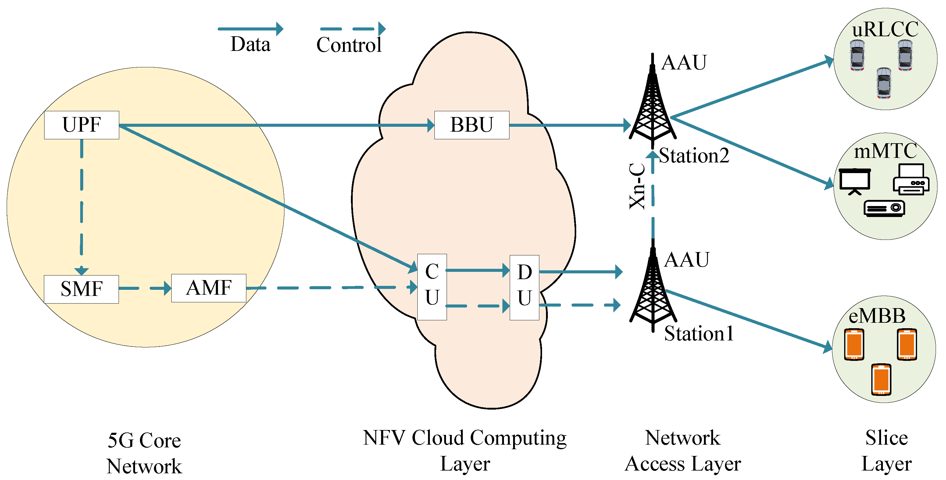
Network function virtualization and slice technique are the core technologies for the 5G communication system. The CU-DU separation architecture based on these technologies makes it possible to flexibly network for different scenarios. Figure 1 plots a 5G network architecture. Station 1 connects to the DU, DU then connects to CU, and CU connects to the 5G core network. Station 2 connects to the BBU indirectly, and the BBU connects to the 5G core network. Because of the dividing of the user plane and the control plane in 5G, the data stream is divided into the actual data stream and the control signaling stream. The solid line refers to the actual stream from the user plane function (UPF) to the CU of station 1 and the BBU of station 2. Then, the dotted line refers to the control signaling from the UPF to the session management function (SMF), then from the SMF to the access and mobility management function (AMF), and then from the AMF to the CU of station 1.

Three scenarios, i.e., eMBB, mMTC, and uRLLC, are considered in this paper, and one slice serves one application scenario. Thus, three slices corresponding to these three 5G scenarios are considered in this paper. The mMTC scenario focuses on the number of connections, and it does not require low latency strictly, such as the Internet of Things users. It can apply the CU and DU separation scheme, so the user in this slice is appropriately connected to the base station 1, as shown in Figure 1. The eMBB scenario focuses on the peaking rate, capacity, and spectrum efficiency and requires low latency, such as for mobile users. It is more appropriate for taking the CU and DU setting together scheme, so the user in this slice is connected to base station 2. The uRLLC focuses on ultra-reliability and low-latency communication, such as the vehicle network. It is most suitable for adopting the CU and DU setting together, so the user in this slice is connected to base station 2.

This means that different slices and different users have different demands for communication resources. Moreover, resource allocation has a clear hierarchical relationship. The base stations allocate resources to the slices, and then the slices allocate resources to the users contained in this slice. This hierarchy brings great challenges to resource allocation. An efficient resource allocation strategy is crucial for improving resource utilization and, thus, improving the economic benefits of operators. Therefore, we proposed a bi-level resource allocation model in which the NFV clouding computing makes the 5G base station allocate the sub-channels and power sources to the three slices, and the slices allocate the sub-channels and power resources obtained from the base station to their users.

Specifically, let $U_n=\{1,2,...u_n\}$ denote the users in the nth slice, where $n=1,2,3$ and $u_n$ are the number of users. We assume that there are K sub-channels and denote the set of sub-channels as $\mathbb{k}=\{1,2,3,...,K\}$. In the upper-level resources allocation of the base station to the slices, the upper-level optimization variables include power allocation $\mathbf{P}={\left(p_n\right)}_{1\times 3}$ and sub-channel allocation $\mathbf{V}={\left(v_{n,k}\right)}_{1\times (3·K)}$. $p_n$ is the power allocated to the nth slice, and $v_{n,k}=1$ denotes that the kth sub-channel is allocated to the nth slice, otherwise $v_{n,k}=0$. When the base station’s allocation of resources ($\mathbf{P},\mathbf{V}$) to the slices has been given, we can obtain the number $K^n$ of sub-channel resource allocated by the base station to the nth slice. In the lower-level resource allocation of the slices to their users, the lower-level optimization variables contain the power allocation $\tilde{\mathbf{P}}=({\tilde{\mathbf{P}}}^1,{\tilde{\mathbf{P}}}^2,{\tilde{\mathbf{P}}}^3)$, with ${\tilde{\mathbf{P}}}^n={\left(p_k\right)}_{1\times K^n}$, sub-channel allocation for users $\tilde{\mathbf{V}}=({\tilde{\mathbf{V}}}^1,{\tilde{\mathbf{V}}}^2,{\tilde{\mathbf{V}}}^3)$, with ${\tilde{\mathbf{V}}}^n={\left(v_{n,u,k}\right)}_{1\times (u_n·K^n)}$, $n=1,2,3$. $p_k$ refers to the power allocated to the kth sub-channel, and $v_{n,u,k}\in \{0,1\}$ refers to the sub-channel allocation. $v_{n,u,k}=1$ denotes that the kth sub-channel is allocated to the uth user in the nth slice, otherwise, $v_{n,u,k}=0$.

3.2. Upper-Level Optimization: 5G Base Stations Allocate Resources to the Slices

The upper-level optimization problem of the bi-level model refers to the base stations allocating the sub-channels and power resources to the slices. The slices apply these resources to customize the service. The 5G operator benefits from the tenants which maintain the slice. The upper-level optimization aims to optimize the benefit of the operator and improve resource utilization and cover more users. Thus, it can be given as:

$$\begin{array}{cc}\hfill \underset{\mathbf{P},\mathbf{V}}{max}& \sum _{n=1}^3{c}_n\sum _{k\in \mathbb{k}}{v}_{n,k}{R}_{n,k}+\lambda \sum _{n=1}^3\sum _{u\in U_n}{b}_{n,u}\hfill \\ \hfill & \mathrm{s}.\mathrm{t}.\sum _n{p}_n\le P_{total}\hfill \\ \hfill & \sum _n{v}_{n,k}\le 1.\hfill \end{array}$$

(1)

where $c_n$ ($c_n>0$) is the unit prices of the nth slice, and $P_{total}$ is the total power resource that the NFV cloud computing layer can be allocated. $R_{n,k}={\sum }_{u\in U_n}{v}_{u,n,k}{R}_{n,u,k}$ is the rate in the nth slices on the kth sub-channel. $R_{n,u,k}$ is the rate of user u in the nth slices obtained on the kth sub-channel, which is given by the resource allocation scheme in the lower-level optimization task. The first term of the objective is the total revenue, and the second term is the total number of covered users. $\lambda$ is a parameter that is used to balance the revenue and the number of covered users.

The first constraint means that the allocating power cannot exceed the total power, and the second constraint means that each sub-channel only can be allocated to one slice at most. Additionally, $b_{n,u}\in \{0,1\}$ denotes the connection identifier that is given by the lower-level optimization task. It is given a detailed description in Section 3.3. The sub-channel allocation $\mathbf{V}$ is discrete, but the power allocation $\mathbf{P}$ is continuous. Therefore, the upper-level optimization problem is a complex constrained mixed variable optimization problem.

3.3. Lower-Level Optimization: Slices Allocate Resources to Their Users

The lower-level optimization of the proposed bi-level resource allocation model is that the slices further allocate the sub-channel and power resources obtained from the based stations to their users. Since different slices correspond to different scenarios, the resource allocation of each slice is relatively independent, we allocate the resources of each slice, respectively. The sub-channel and power resources are allocated according to the channel gain and desired rate of the users. The lower-level optimization task aims to optimize the service equity of all users in each slice. Thus, the lower-level optimization problem can be given as:

$$\begin{array}{cc}\hfill \underset{\tilde{\mathbf{P}},\tilde{\mathbf{V}}}{max}& \sum _{n=1}^3\sum _{u\in U_n}{b}_{n,u}{\left(\frac{\sum _{k\in \mathbb{k}}{v}_{n,u,k}{R}_{n,u,k}}{r{d}_{n,u}}\right)}^{\frac{\sum _{k\in \mathbb{k}}{v}_{n,u,k}{p}_{n,u,k}}{p_n}}\hfill \\ \hfill & \mathrm{s}.\mathrm{t}.p^{min}{v}_{n,u,k}\le p_{n,u,k}{v}_{n,u,k}\le p^{max}{v}_{n,u,k}\hfill \\ \hfill & \sum _{u\in U_n}^{}\sum _{k\in \mathbb{k}}{v}_{n,u,k}{p}_{n,u,k}\le p_n\hfill \\ \hfill & v_{n,k}=\sum _{u\in U_n}{v}_{n,u,k}\hfill \end{array}$$

(2)

where $R_{n,u,k}$ is the rate of user u in the nth slice obtained on the kth sub-channel. It is calculated by

$$R_{n,u,k}=w\ast log\left(1+\frac{p_{n,u,k}\times v_{n,u,k}\times g_{n,u,k}}{{\sigma }^2}\right),$$

(3)

where w is the bandwidth of the sub-channel and ${\sigma }^2$ is the noise power, ${\mathbf{G}}^n={\left(g_{n,u,k}\right)}_{1\times (u_n·K)}$ is the channel gain matrix, and $g_{n,u,k}$ is the channel gain on the sub-channel k between the user u in the nth slice and the 5G base station, which is calculated as $g_{n,u,k}={10}^{-PL\left(d_{n,u}\right)/10}$, where $PL(.)$ is the path loss function with a shadow fading that follows a normal distribution, according to the actual scene, and $d_{n,u}$ is the distance between the user and the base station. ${\mathbf{Rd}}^n={\left(r{d}_{n,u}\right)}_{1\times u_n}$ is the desired rate of the users in the nth slice.

The first constraint of problem (2) makes that the power allocated to each sub-channel must be in the range $p^{min}$ and $p^{max}$. The second constraint of problem (2) states that the power allocated to the users in the nth slice cannot exceed the power allocated to the nth slice. The third constraint means that each sub-channel only can be allocated to one user at most. The connection identifier $b_{n,u}$ is calculated as follows. $b_{n,u}=1$ represents that the uth user is connecting and its communication rate meets the minimum communication requirement of the nth slice, otherwise, $b_{n,u}=0$. That is

$$b_{n,u}=\left\{\begin{array}{cc}\hfill 1& \mathrm{if}\sum _{k\in \mathbb{k}}{R}_{n,u,k}{v}_{n,u,k}\ge R_n^{min};\hfill \\ \hfill 0& \mathrm{otherwise}.\hfill \end{array}\right.$$

(4)

where $R_n^{min}$ is the minimum rate promised by joining the nth slice.

The lower-level optimization variable $\tilde{\mathbf{P}}$ is continuous, and $\tilde{\mathbf{V}}$ is 0–1 discrete optimization variables. The lower-level optimization problem is also a constrained mixed variable optimization problem. Therefore, the proposed bi-level resource allocation model is a nonlinear constraint mixed-discrete variable optimization problem. Additionally, in the actual 5G application scenarios, the services that the slices request change rapidly, which puts forward higher requirements and challenges for the speed of the algorithm. Thus, we need to present a fast resource allocation algorithm. We use a reinforcement learning method to solve the proposed bi-level resource allocation model in this paper.

In summary, the bi-level resource allocation model can be formulated as the following mathematical model.

$$\begin{array}{cc}\hfill \underset{\mathbf{P},\mathbf{V},\tilde{\mathbf{P}},\tilde{\mathbf{V}}}{max}& \sum _{n=1}^3{c}_n\sum _{k\in \mathbb{k}}{v}_{n,k}{R}_{n,k}+\lambda \sum _{n=1}^3\sum _{u\in U_n}{b}_{n,u}\hfill \\ \hfill & \mathrm{s}.\mathrm{t}.\sum _n{p}_n\le P_{total},\hfill \\ \hfill & \sum _n{v}_{n,k}\le 1,\hfill \\ \hfill & \tilde{\mathbf{P}},\tilde{\mathbf{V}}\in arg\underset{\tilde{\mathbf{P}},\tilde{\mathbf{V}}}{max}\left\{\sum _{n=1}^3\sum _{u\in U_n}{b}_{n,u}{\left(\frac{{\sum }_{k\in \mathbb{k}}{v}_{n,u,k}{R}_{n,u,k}}{r{d}_{n,u}}\right)}^{\frac{{\displaystyle \sum _{k\in \mathbb{k}}}{v}_{n,u,k}{p}_{n,u,k}}{p_n}},\right.\hfill \\ \hfill & \mathrm{s}.\mathrm{t}.p^{min}{v}_{n,u,k}\le p_{n,u,k}{v}_{n,u,k}\le p^{max}{v}_{n,u,k},\hfill \\ \hfill & \sum _{u\in U_n}^{}\sum _{k\in \mathbb{k}}{v}_{n,u,k}{p}_{n,u,k}\le p_n,\hfill \\ \hfill & \left.v_{n,k}=\sum _{u\in U_n}{v}_{n,u,k}\right\}.\hfill \end{array}$$

(5)

4. Resource Allocating Based on Reinforcement Learning

4.1. The Flow of the Proposed Resource Allocation Algorithm

Reinforcement learning can give a better resource allocation scheme with a certain real-time computing resource, which has been widely used in practice. However, the selection of the architecture and the components of reinforcement learning has a great impact on the performance of the algorithm. It is necessary to choose the appropriate reinforcement learning architecture for different problems. We employ MATD3 for the upper-level resources allocation and DCTD3 for the lower-level resources allocation, according to the challenges of the proposed resource allocation model. In the actual scenario, we must ensure mutual isolation and security between slices, so we do not use multiple agents in the process of slice resource allocation to users, but train one agent for each slice for resource allocation.

Figure 2 plots the flow of the proposed resource allocation process. The MATD3 reinforcement learning algorithm contains two agents. One agent is for the base station allocating the discrete sub-channel resources ($\mathbf{V}$) to the slice, and the other agent is for the base station allocating continuous power resources ($\mathbf{P}$) to the slice. DCTD3 is employed for the lower-level optimization task, which enables each slice to simultaneously allocate the discrete sub-channel resources (${\tilde{\mathbf{V}}}^n$) and continuous power resources (${\tilde{\mathbf{P}}}^n$) obtained from the base station to its users. The agent in the lower level is trained according to the reward of the lower-level objective. After the resources are allocated to users by the lower-level slices, the agents in the upper level will get a reward by calculating the upper-level objective according to the results of the lower-level resource allocation.

4.2. The Upper-Level Resource Allocation by Using MATD3

How to effectively and accurately define the components, i.e., state, environment, action, and reward, of reinforcement learning is the key to applying reinforcement learning to solve practical problems. We will give a detailed description of the components of reinforcement learning. In the upper-level optimization, the power allocation is a continuous variable and the sub-channel allocation is a 0-1 discrete variable. In addition, there are more and more slices in the actual scenario under CD-DU separation. The increase in dimension brings challenges to the convergence of reinforcement learning. Therefore, MATD3 with two agents is employed for the upper-level resource allocation. Algorithm 1 provides the pseudo-code flow of the algorithm. The first agent is used to allocate sub-channels resources, and the second agent is to allocate power resources. Additionally, the two agents cooperate for the same upper-level objective.

Algorithm 1 MATD3 for the upper-level optimization.

1: for agent m = 1 to 2 do 2:    Randomly initialize two current critic networks $Q_1({\mathbf{S}}_{t,m},{\mathbf{A}}_t\mid {\theta }_{m,1}^Q)$, $Q_2({\mathbf{S}}_{t,m},{\mathbf{A}}_t\mid {\theta }_{m,2}^Q)$ and one current actor network $\mu ({\mathbf{S}}_{t,m}\mid {\theta }_m^{\mu })$ with weights ${\theta }_{m,1}^Q$, ${\theta }_{m,2}^Q$ and ${\theta }_m^{\mu }$. 3:    Initialize target critic networks $Q_1^{\prime }({\mathbf{S}}_{t,m},{\mathbf{A}}_t\mid {\theta }_{m,1}^{Q^{{}^{\prime }}})$, $Q_2^{\prime }({\mathbf{S}}_{t,m},{\mathbf{A}}_t\mid {\theta }_{m,2}^{Q^{{}^{\prime }}})$ and target actor ${\mu }^{\prime }({\mathbf{S}}_{t,m}\mid {\theta }_m^{{\mu }^{{}^{\prime }}})$ with weights ${\theta }_{m,1}^{Q^{{}^{\prime }}}⟵$${\theta }_{m,1}^Q$, ${\theta }_{m,2}^{Q^{{}^{\prime }}}⟵$${\theta }_{m,2}^Q$, ${\theta }_m^{{\mu }^{{}^{\prime }}}⟵$${\theta }_m^{\mu }$. 4: end for 5: for episode = 1 to $E_{max}$ do 6:    Initialize the state of the agents ${\mathbf{S}}_t={({\mathbf{S}}_{t,1},{\mathbf{S}}_{t,2})}_{t=0}$. 7:    for t = 1 to $T_{max}$ do 8:      Select the action ${\mathbf{a}}_{t,m}=\mu ({\mathbf{S}}_{t,m}\mid {\theta }_m^{\mu })+{ϵ}_{}$ by the current actor network, $m=1,2$. 9:      The first agent executes action ${\mathbf{a}}_{t,1}$ to allocate sub-channels to slices. 10:      The second agent executes action ${\mathbf{a}}_{t,2}$ to allocate power resource to slices. 11:      Observe reward $r_t$ and observe new state ${\mathbf{S}}_{t+1}=({\mathbf{S}}_{t+1,1},{\mathbf{S}}_{t+1,2})$. 12:      Store transition $({\mathbf{S}}_t,{\mathbf{A}}_t,r_t,{\mathbf{S}}_{t+1})$ in D. 13:      Sample a random minibatch of S transition $({\mathbf{S}}_i,{\mathbf{A}}_i,r_i,{\mathbf{S}}_{i+1})$ from D. 14:      Set ${\mathbf{S}}_t={\mathbf{S}}_{t+1}$. 15:      for agent m = 1 to 2 do 16:         Calculate the value of $Q_{target}^{\prime }$ of mth agent according to Equation (13). 17:         Update the current critic networks by minimizing the loss according to Equation (14). 18:         Update the current actor network according to Equation (15) or Equation (16). 19:         Update the target critic networks according to Equation (17). 20:         Update the target actor network according to Equation (18). 21:      end for 22:    end for 23: end for

4.2.1. State

At each time-step, the state of the mth agent of MATD3 consists of the following four aspects in this paper.

• The average channel gain ${\mathbf{G}}^{av}$: ${\mathbf{G}}^{av}={\left(g_{n,k}\right)}_{1\times (3·K)}$ with $g_{n,k}$ is the average channel gain of users is the nth slice on the kth sub-channel, $g_{n,k}=\frac{{\sum }_{u=1}^{u_n}{g}_{n,u,k}}{u_n}$.
• The percentage of the request rate ${\mathbf{PR}}^{rate}$: ${\mathbf{PR}}^{rate}={\left(p{r}_n^{rate}\right)}_{1\times 3}$, with $p{r}_n^{rate}$ being the percentage of the request rate of the nth slice. $p{r}_n^{rate}=\frac{{\sum }_{u=1}^{u_n}r{d}_{n,u}}{{\sum }_n{\sum }_{u=1}^{u_n}r{d}_{n,u}}$.
• The sub-channels assignment $\mathbf{V}\left(t\right)$ at time t.
• The power resource allocation $\mathbf{P}\left(t\right)$ at time t.

We denote ${\mathbf{S}}_{t,m}=\left({\mathbf{G}}^{av},{\mathbf{PR}}^{rate},\mathbf{V}\left(t\right),\mathbf{P}\left(t\right)\right)$ as the state of the mth agent and ${\mathbf{S}}_t=\left({\mathbf{S}}_{t,1},{\mathbf{S}}_{t,2}\right)$ as the state of the two agents at time t.

4.2.2. Multi-Agent Actor and Critic Networks

The action ${\mathbf{a}}_{t,1}={\left(a_{n,k}\left(t\right)\right)}_{1\times (3·K)}$ of the first agent is the action regarding the sub-channels allocation for three slices at time t. For each k sub-channel, we assign it to the $n^{\ast }$ slice with the maximum value, that is, $n^{\ast }=arg\underset{n}{max}\left(a_{n,k}\left(t\right)\right)$—the value of $v_{n^{\ast },k}$ is set to 1, and the value of $v_{n,k}$ for the other slice is set to 0 at time $t+1$. Therefore, the action ${\mathbf{a}}_{t,1}$ impacts the sub-channel allocation $\mathbf{V}(t+1)$ of the state of the two agents.

The action ${\mathbf{a}}_{t,2}={\left(a_n\left(t\right)\right)}_{1\times 3}$ of the second agent regards the power allocation for the three slices at time t. At each time-step, the action of power increases or decreases $\nabla p_1$ at time t, where $\nabla p_1$ is the power action bound at time t in the upper-level optimization. The power allocation $\mathbf{P}(t+1)$ is computed with the action of the second agent by Equation (6):

$$\mathbf{P}(t+1)=\mathbf{P}\left(t\right)+{\mathbf{a}}_{t,2}\ast \nabla p_1.$$

(6)

Therefore, the actions ${\mathbf{a}}_{t,2}$ will impact the state $\mathbf{P}(t+1)$ of the agents and the entire environment.

Two current critic networks $Q_1({\mathbf{S}}_{t,m},{\mathbf{A}}_t\mid {\theta }_{m,1}^Q)$ and $Q_2({\mathbf{S}}_{t,m},{\mathbf{A}}_t\mid {\theta }_{m,2}^Q)$ with weights ${\theta }_{m,1}^Q$, ${\theta }_{m,2}^Q$ are randomly initialized, which are used to approximate the Q-function for the mth agent in MATD3. Moreover, we initialize one current actor network $\mu ({\mathbf{S}}_{t,m}\mid {\theta }_m^{\mu })$ with weights ${\theta }_{m,1}^Q$ for each mth agent as shown in line 2 of Algorithm 1, where ${\mathbf{A}}_t=\left({\mathbf{a}}_{t,1},{\mathbf{a}}_{t,2}\right)$. The current actor network chooses a deterministic action based on the state ${\mathbf{S}}_{t,m}$ at time t by using the deterministic policy gradient. Then, the action ${\mathbf{a}}_{t,m}$ of the mth agent at time t can be given as:

$${\mathbf{a}}_{t,m}=\pi \left({\mathbf{S}}_{t,m}\right)=\mu \left({\mathbf{S}}_{t,m}\mid {\theta }_m^{\mu }\right)+{ϵ}_1.$$

(7)

where ${ϵ}_1\sim \mathcal{N}(0,{\sigma }_1^2\left(t\right))$ is a normal random noise. It is used to explore more movements. The variance of this noise decreases with the number of training epochs, that is, ${\sigma }_1^2(t+1)=\eta {\sigma }_1^2\left(t\right)$, where $\eta$ is a constant less than one. The action is compressed to $(-1,1)$ by the Tanh activation function in the actor network.

Moreover, we initialize two critic target networks, $Q_1^{\prime }\left({\mathbf{S}}_{t,m},{\mathbf{A}}_t^{\prime }|{\theta }_{m,1}^{Q^{\prime }}\right)$ and $Q_2^{\prime }\left({\mathbf{S}}_{t,m},{\mathbf{A}}_t^{\prime }|{\theta }_{m,2}^{Q^{\prime }}\right)$, and one target actor network, ${\mu }^{\prime }\left({\mathbf{S}}_{t,m}\mid {\theta }_m^{{\mu }^{\prime }}\right)$, where ${\mathbf{A}}_t^{\prime }=\left({\mathbf{a}}_{t,1}^{\prime },{\mathbf{a}}_{t,2}^{\prime }\right)$. The parameters ${\theta }_{m,1}^{Q^{\prime }}$, ${\theta }_{m,2}^{Q^{\prime }}$ and ${\theta }_m^{{\mu }^{\prime }}$ are initialized with that of the corresponding current actor networks. The action ${\mathbf{a}}_{t,m}^{\prime }$ is given as:

$${\mathbf{a}}_{t,m}^{\prime }={\mu }^{\prime }\left({\mathbf{S}}_{t+1,m}\mid {\theta }_m^{{\mu }^{\prime }}\right)+{ϵ}_1.$$

(8)

4.2.3. Reward

After the two agents execute theirs action ${\mathbf{a}}_{t,m}$, the environment state is changed from ${\mathbf{S}}_{t,m}$ to ${\mathbf{S}}_{t+1,m}$. The mth agent gets a reward $r_{t,m}$ from the environment, $m=1,2$. In upper-level optimization, two agents are assigned to allocate sub-channels and power resources for the same upper-level optimization objective. Therefore, we set the same reward function for these two agents at time t, that is, $r_{t,1}=r_{t,2}$, according to the objective function and the constraint violation of the upper-level optimization (1).

$$r_{t,m}=\sum _n{c}_n\sum _k{v}_{n,k}{R}_{n,k}+\lambda \sum _n\sum _{u\in U_n}{b}_{n,u}\left(t\right)-\iota \varrho ,m=1,2.$$

(9)

where the $\varrho$ is the degree of constraint violation and $\iota$ is the penalty coefficient. Therefore, the total reward $R_{t,m}^{total}$ of the mth agent can be given as

$$R_{t,m}^{total}=\sum _{\tau =0}^T{\gamma }^{\tau }{r}_{t+\tau ,m}.$$

(10)

where $\gamma \in [0,1]$ is a discount factor. The Q-value function based on the Belman function can evaluate the expected total return per action. It can be denoted as follows

$$\begin{array}{cc}\hfill Q^{\pi }(S_{t,m},a_{t,1},a_{t,2})& =E_{\pi }\left[R_t^{total}\mid S_{t,m},a_{t,1},a_{t,2}\right]\hfill \\ \hfill & =E_{\pi }\left[\sum _{\tau =0}^T{\gamma }^{\tau }{r}_{t+\tau ,m}\mid S_{t,m},a_{t,1},a_{t,2}\right]\hfill \\ \hfill & =E_{\pi }\left[r_{t,m}+\gamma Q^{\pi }(S_{t+1,m},a_{t+1,1},a_{t+1,2})\mid S_{t,m},a_{t,1},a_{t,2}\right].\hfill \end{array}$$

(11)

We select actions ${\mathbf{A}}_t=\left({\mathbf{a}}_{t,1},{\mathbf{a}}_{t,2}\right)$ of agents according to Equation (7) for a given state ${\mathbf{S}}_t$. Then, we execute action ${\mathbf{a}}_{t,m}$ to get the rewards of agents $r_t=\left(r_{t,1},r_{t,2}\right)$ and the new states of the two agents ${\mathbf{S}}_{t+1}=\left({\mathbf{S}}_{t+1,1},{\mathbf{S}}_{t+1,2}\right)$. Transition $({\mathbf{S}}_t,{\mathbf{A}}_t,r_t,{\mathbf{S}}_{t+1})$ is stored in the memory replay D, as shown in line 13 of Algorithm 1.

4.2.4. Training Process of MATD3

We extract samples $({\mathbf{S}}_i,{\mathbf{A}}_i,r_i,{\mathbf{S}}_{i+1})$ from D, with a batch size N for training the networks at each time-step. Figure 3 plots the training process of agent 1 of MATD3. Global information is required to be adopted for training the networks in multiple agents-based reinforcement learning. Therefore, we need to input the actions of all agents into the current critic networks. The parameters of the current critic networks are updated to minimize the loss. The loss function of the jth current critic network of the mth agent is given as

$$L\left({\theta }_{m,j}^Q\right)=\frac{1}{N}\sum _i{\left[y_{i,m}-Q_j\left({\mathbf{S}}_{i,m},{\mathbf{A}}_i|{\theta }_{m,j}^Q\right)\right]}^2,j=1,2.$$

(12)

where $y_{i,m}=r_{i,m}+\gamma Q_{target}^{\prime }$ is an approximation of policy. The values of $Q_{target}^{\prime }$ are the minimum Q-values of the target critic networks $Q_1^{\prime }$ and $Q_2^{\prime }$. That is,

$$Q_{target}^{\prime }=min(Q_1^{\prime }({\mathbf{S}}_{i+1,m},{\mathbf{A}}_i^{\prime }\mid {\theta }_{m,1}^{Q^{\prime }}),Q_2^{\prime }({\mathbf{S}}_{i+1,m},{\mathbf{A}}_i^{\prime }\mid {\theta }_{m,2}^{Q^{\prime }})),$$

(13)

where ${\mathbf{A}}_i^{\prime }=({\mathbf{a}}_{i,1}^{\prime },{\mathbf{a}}_{i,2}^{\prime })$ contains actions of the target actor network of the two agents. Then, the parameters ${\theta }_{m,j}^Q$ of the jth current critic network of the mth agent is updated to minimize the loss function. That is,

$${\theta }_{m,j}^Q\leftarrow argminL\left({\theta }_{m,j}^Q\right),j=1,2.$$

(14)

The parameters of the current actor network of the agents are updated by using a deterministic policy gradient strategy. We can get to the Q-value through any one of the current critic networks, We choose the Q-value from the first current critic network in this paper. Accordingly, we can derive the gradient of the ensemble objective concerning the first agent, i.e., $m=1$ as follows:

$${\nabla }_{{\theta }_1^{\mu }}J=E\left[{\nabla }_{\mathbf{a}}{Q}_1({\mathbf{S}}_{i,1},{\mathbf{a}}_{},{\mathbf{a}}_{i,2}\mid {\theta }_1^Q){\nabla }_{{\theta }_1^{\mu }}\mu ({\mathbf{S}}_{i,1}\mid {\theta }_1^{\mu }){|}_{\mathbf{a}=\mu \left({\mathbf{S}}_{i,1}\right|{\theta }_1^{\mu })}\right].$$

(15)

For the second agent,

$$\begin{array}{c}\hfill {\nabla }_{{\theta }_2^{\mu }}J=E\left[{\nabla }_{\mathbf{a}}{Q}_1({\mathbf{S}}_{i,2},{\mathbf{a}}_{i,1},{\mathbf{a}}_{}\mid {\theta }_1^Q){\nabla }_{{\theta }_2^{\mu }}\mu ({\mathbf{S}}_{i,2}\mid {\theta }_2^{\mu }){|}_{\mathbf{a}=\mu \left({\mathbf{S}}_{i,2}\right|{\theta }_2^{\mu })}\right].\end{array}$$

(16)

In this paper, we use the Adam optimizer [49] with a learning rate of $\alpha =0.001$ and ${\beta }_1=0.9$, ${\beta }_2=0.999$ to update the parameters of the current actor networks. The learning rate $\alpha$ is allowed to adjust during the training phase.

After an epoch of training, we update the parameters of the target critic networks of the mth agent as follows:

$${\theta }_{m,j}^{Q^{\prime }}⟵\varsigma {\theta }_{m,j}^Q+(1-\varsigma ){\theta }_{m,j}^{Q^{\prime }},j=1,2.$$

(17)

The parameters of the target actor network of the mth agent are updated as:

$${\theta }_m^{{\mu }_{}^{\prime }}⟵\varsigma {\theta }_m^{{\mu }_{}}+(1-\varsigma ){\theta }_m^{{\mu }_{}^{\prime }},$$

(18)

where $\varsigma <1$ is a smaller constant to update target networks. The calculation of reward in upper-level optimization depends on the lower-level optimization scheme given by the actor network of the lower-level optimization.

4.3. The Lower-Level Resource Allocation by Using DCTD3

Because slices are securely isolated from each other and there is an interaction between agents in multi-agent reinforcement learning, we use only one agent to complete discrete sub-channel resource allocation and continuous power resource allocation from slices to users. Therefore, we employ DCTD3 for this resource allocation model to solve the problem of simultaneously allocating discrete resources and continuous resources. Each slice corresponds to an agent.

To deal with the resource allocation of the nth slice, we denote the state of the agent in the nth slice as ${\mathbf{S}}_t^n=({\mathbf{G}}^n,{\mathbf{Rd}}^n,{\tilde{\mathbf{V}}}^n\left(t\right),{\tilde{\mathbf{P}}}^n\left(t\right))$, where ${\mathbf{G}}^n={\left(g_{n,u,k}\right)}_{1\times (u_n·K^n)}$ is the channel gain vector about the users on these $K^n$ sub-channels, $g_{n,u,k}$ is the channel gain on the sub-channel k between the user u in the nth slice and the 5G base station, and ${\mathbf{Rd}}^n={\left(r{d}_{n,u}\right)}_{1\times u_n}$ is the desired rate of the users in the nth slice. ${\tilde{\mathbf{V}}}^n\left(t\right)$ and ${\tilde{\mathbf{P}}}^n\left(t\right)$ are the sub-channel allocation and power allocation in the nth slice at time t, respectively.

The action of the nth agent consists of two parts: ${\mathbf{a}}_t^n=({\mathbf{a}}_1^n\left(t\right),{\mathbf{a}}_2^n\left(t\right))$. It is compressed to $(-1,1)$ by using the Tanh function. It also adds a noise, as used in MATD3 for exploration. The action ${\mathbf{a}}_1^n\left(t\right)={\left(a_{u,k}^{n,1}\left(t\right)\right)}_{1\times (u_n·K^n)}$ is about sub-channels allocation for users in the n slice. For each sub-channel k, we assign it to the $u^{\ast }$ user with the maximal value, that is, $u^{\ast }=arg\underset{u}{max}\left(a_{u,k}^{n,1}\left(t\right)\right)$, and the $v_{n,u\ast ,k}$ is set to 1 at time $t+1$. The action ${\mathbf{a}}_2^n\left(t\right)={\left(a_k^{n,2}\left(t\right)\right)}_{1\times \left(K^n\right)}$ is about power allocation for $K^n$ sub-channels. At each time-step, the action of power increases or decreases $\nabla p_2$ at time t, where $\nabla p_2$ is the power action bound at time t in the lower-level optimization.

$${\mathbf{P}}^n(t+1)={\mathbf{P}}^n\left(t\right)+{\mathbf{a}}_2^n\left(t\right)\nabla p_2.$$

(19)

Therefore, the discrete subchannels resource and continuous power resources can be allocated together by using only one agent.

The state of the environment changes according to these processed actions, that is, ${\mathbf{S}}_t^n$ becomes ${\mathbf{S}}_{t+1}^n$. First of all, we need to generate training samples, that is, to extract a certain batch of training samples of reinforcement learning and store it in experience replay. The states of the input neural network are composed of the channel gain, desired rate, and allocated power. After taking enough samples, we start to train the critic and actor networks. The reward is defined according to the objective and constraint violation of the lower-level optimization (2) at time t:

$$r_t^n=\sum _{u\in U_n}^{}{b}_{n,u}\left(t\right){\left(\frac{{\sum }_k{R}_{n,u,k}\left(t\right)}{r{d}_{n,u}}\right)}^{({\sum }_k{p}_k\left(t\right)\ast v_{n,u,k})/p_n}-\iota \varrho .$$

(20)

where the $\varrho$ is the degree of constraint violation and $\iota$ is the penalty coefficient.

The training process is similar to MATD3 in the upper-level optimization on the whole, except that, in the critic network, we only need the actions of the current agent, but not the actions of other agents. Therefore, we extract samples with a batch size N, and the update formula through gradient ascent of the actor network of each agent with parameter ${\theta }_{}^{\mu }$ in the nth slice is as follows

$$\begin{array}{c}\hfill {\nabla }_{{\theta }^{\mu }}J=E\left[{\nabla }_{{\mathbf{a}}_i^n}{Q}_1({\mathbf{S}}_i^n,{\mathbf{a}}_i^n\mid {\theta }_1^Q){\nabla }_{{\theta }_1^{\mu }}\mu ({\mathbf{S}}_i^n\mid {\theta }_1^{\mu })\right].\end{array}$$

(21)

Then, the loss that we want to reduce of the agent’s current critic networks with parameter ${\theta }_1^Q,{\theta }_2^Q$ in the nth slice can be calculated as

$$L\left({\theta }_j^Q\right)=\frac{1}{N}{\left[y_i-Q_j({\mathbf{S}}_i^n,{\mathbf{a}}_i^n\mid {\theta }_j^Q)\right]}^2,j=1,2.$$

(22)

Additionally, the target networks are updated by Equations (17) and (18), the same as MATD3 for the upper-level optimization. In case of similar problems, we can input its state into the actor network to a good solution for lower optimization by iterating a certain time. We then give the lower allocation scheme to the upper optimization.

5. Simulation Results and Analysis

To demonstrate the effectiveness of the proposed model and algorithm, we conducted a lot of simulated training. We assumed that there were two stations deployed on the center of a square region 400 m × 400 m. They jointly served three slices, corresponding to different application scenarios (mMTC, eMBB, uRLLC) of 5G under CU-DU separation. We also assumed that there were two users in the first slice, three users in the second slice, and four users in the third slice. The desired rates $r{d}_{1,u}$, $r{d}_{2,u}$, $r{d}_{3,u}$ of each of the users are randomly initialized in $[3,6]$ MB/s, $[6,9]$ MB/s and $[9,12]$ MB/s, respectively. The path loss model used in this paper is $22lo{g}_{10}\left(d\right)+28+20lo{g}_{10}\left(f_c\right)+{\sigma }_{SF}$, where d is the distance between the user and the connected base station and $f_c$ is the central frequency of the 5G band, which is set to $f_c$ = 3 GHz. Because the user’s channel gain for each sub-channel is constantly changing in real scenarios, we re-initialize the normally distributed variables ${\sigma }_{SF}\sim \mathcal{N}(0,3^2)$ for each epoch. The learning rate of the proposed algorithm is set to 0.0001, memory capacity D = 10,000, and batch size $N=64$. Each network of agents has one hidden layer with 128 dimensions. All simulation results are provided with pytorch-gpu 1.12.1 on Python 3.8 platform. A summary of the parameters is listed in

Table 1. Summary of simulation parameters.

Notation	Description
$u_1,u_2,u_3$	2, 3, 4
$P^{total}$	12 W
$R_1^{min}$, $R_2^{min}$, $R_3^{min}$	3 MB/s, 6 MB/s, 9 MB/s
w	180 kHz
$\gamma$	0.99
Noise power spectral density ${\sigma }^2$	−174 dBm/Hz
Pathloss	$22lo{g}_{10}\left(d\right)+28+20lo{g}_{10}\left(f_c\right)+{\sigma }_{SF}$
Fading shadow ${\sigma }_{SF}$	${\sigma }_{SF}\sim \mathcal{N}(0,3^2)$
Rate unit price $c_1,c_2,c_3$	0.5, 0.3, 0.2
$\lambda$	3
$p_{}^{min},p_{}^{max}$	120 mW, 800 mW
$\nabla p_1,\nabla p_2$	100 mW, 50 mW
K	20
$\varsigma$	0.998
$\eta$	0.9999

.

5.1. The Performance of MATD3 for the Upper-Level Resource Allocation

The $E_{max}$ was set to 2500, and the $T_{max}$ was set to 50 in upper-level optimization. Figure 4 shows the training results of MATD3 for the upper-level resource allocation. Specifically, Figure 4a plots the total reward vs the epoch. From this figure, we can see that the total reward in each epoch of the agents converges after 2250 epochs. Figure 4b,c plot the loss values of the first agent and the second agent, respectively. From this figure, we can see that the loss function of the first agent to allocate sub-channels dropped off by 1450 epochs, and by 2300 epochs, it was already below 0.1. The loss function of the second agent dropped by 1400 epochs, and by 2250 epochs, it was already below 0.1. From these figures, we can see that the proposed algorithm has better convergence.

In addition, due to the randomness of reinforcement learning, the trained agents may not be able to explore high-value areas. High-value areas can be regarded as optimal solutions in reinforcement learning. We conducted the proposed algorithm 10 times independently to verify the stability of the proposed algorithm by different random number seeds.

Table 2. Statistical analyses of the rewards and the loss of the agents.

Reward			Loss of Agent 1			Loss of Agent 2
Best	Mean	Variance	Best	Mean	Variance	Best	Mean	Variance
49.5	47.97143	3.23238	0.001	0.71429	0.0981	0.001	0.52357	0.0487

lists the best value, the mean value, and the value of the variance of the reward and the loss of the critic networks of agents. The results from the statistical analyses yielded that the proposed algorithm is robust and accurate.

We conducted the proposed algorithm with different learning rates in the Adam optimizer and compared it with the MADDPG algorithm and nested bi-level evolutionary algorithm (NBLEA) [50] to further investigate the performance of the proposed algorithm. The Adam optimizer is used to optimize the parameters of the current critic networks of MATD3. The learning rates of the Adam optimizer were set to 0.001, 0.0001, and 0.00001, respectively. After the cumulative reward converges, we saved the actor neural network, which can quickly get a better solution through a simple calculation. Figure 5 shows the comparison results for 10 independent runs. From this figure, we can see that MATD3, with a learning rate of 0.0001, can obtain a promising result. The results obtained by NBLEA are superior to that of MATD3. Nested evolutionary algorithms are a popular approach for handling bi-level problems, where lower-level optimization problem is solved, corresponding to each upper-level member. Though NBLEA is superior to MATD3, in terms of accuracy, nested strategies are computationally very expensive.

5.2. The Performance of DCTD3 for the Lower-Level Optimization

The parameter $T_{max}$ of DCTD3 was set to 30 in all slices. The $E_{max}$ was set to 2000 in slice 1, 5000 in slice 2, and 10,000 in slice 3. We interacted with the environment and collected 9000 samples and stored them in the experience replay. Figure 6 plots the total rewards of the agent in different slices. Specifically, Figure 6a plots the total reward of the agent in the first slice. This figure shows that a higher reward is achieved in about 50 epochs. Figure 6b plots the total reward of the agent in the second slice. This figure shows that a higher reward is achieved in less than 1000 epochs. The total reward of agent in the third slice is shown in Figure 6c. From this figure, we can see that we can obtain a higher reward with about 1000 epochs. This means that the proposed algorithm can obtain a promising result with a smaller number of iterations.

Figure 7 plots the values of the loss functions of the critic networks, which are used to allocate the resources to the users. From this figure, we can see that the values of the loss functions gradually decrease with the increase in the number of training epochs. In the first slice, the loss of DCTD3 critic networks converges when the training epoch was about 2000 with 64 batch size samples, as shown in Figure 7a. In the second slice, the loss converges when the training epoch was about 2000 epochs, as shown in Figure 7b. The training epoch needed to be at 3000 epochs for loss converges for the third slice, as shown in Figure 7c. In these three slices, the different epochs to achieve loss convergence were caused by the different numbers of users in the slices and the different numbers of allocated sub-channels. The loss functions of all agents could achieve convergence. After the training, we only saved the actor-network of each slice. We could input the state into the actor network and iterate it for a certain number of time steps to quickly get a better resource allocation scheme within a certain time.

6. Conclusions

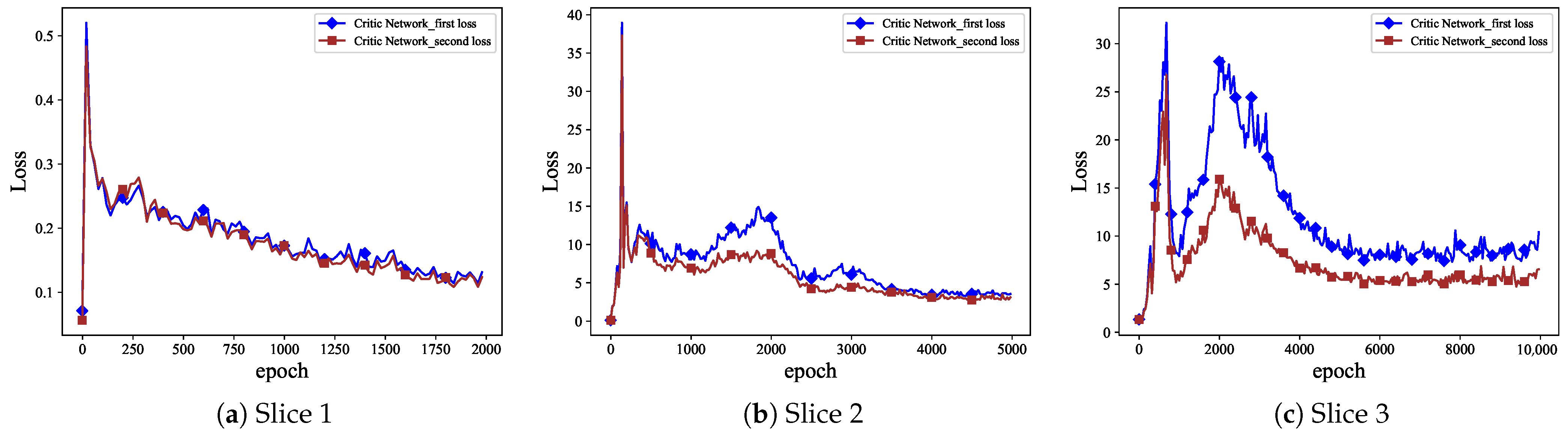
In this paper, we established a bi-level resource allocation model for the 5G wireless communication system under the CU-DU separation architecture. The upper-level optimization is about the base stations allocating the resources to the slices to optimize the operator’s benefits, and the lower-level optimization is about the slices allocating the resource to their users to improve the service equity of all users. In the actual application of this scenario, because the situation in the slice changed rapidly, it required an algorithm that can quickly give a better allocation scheme. Thus, this paper employed MATD3 for the upper-level resource allocation and DCTD3 for the lower-level resource allocation. Finally, we conducted a lot of simulation experiments. The results demonstrated the efficiency and feasibility of the proposed algorithm.

In the future, we will try to study how to allocate different amounts of resource blocks with fixed input action dimensions to realize the training of only one agent for each slice in a real sense. However, due to this kind of reinforcement learning based on neural networks, a different allocation of resource blocks have different dimensions during training, which brings many restrictions in the actual landing. We will make some improvements in this area to make the algorithm generalize better.

References

1. Lv, S.; Xu, X.; Han, S.; Tao, X.; Zhang, P. Energy-Efficient Secure Short-Packet Transmission in NOMA-Assisted mMTC Networks With Relaying. IEEE Trans. Veh. Technol. 2022, 71, 1699–1712. [Google Scholar] [CrossRef]
2. Alsenwi, M.; Tran, N.H.; Bennis, M.; Pandey, S.R.; Bairagi, A.K.; Hong, C.S. Intelligent Resource Slicing for eMBB and URLLC Coexistence in 5G and Beyond: A Deep Reinforcement Learning Based Approach. IEEE Trans. Wirel. Commun. 2021, 20, 4585–4600. [Google Scholar] [CrossRef]
3. Prathyusha, Y.; Sheu, T.L. Coordinated Resource Allocations for eMBB and URLLC in 5G Communication Networks. IEEE Trans. Veh. Technol. 2022, 71, 8717–8728. [Google Scholar] [CrossRef]
4. Askari, L.; Musumeci, F.; Salerno, L.; Ayoub, O.; Tornatore, M. Dynamic DU/CU Placement for 3-layer C-RANs in Optical Metro-Access Networks. In Proceedings of the 2020 22nd International Conference on Transparent Optical Networks (ICTON), Bari, Italy, 19–23 July 2020; pp. 1–4. [Google Scholar] [CrossRef]
5. Baghernia, E.; Sebak, A.R. Millimeter-Wave Wideband Printed Circularly Polarized Antenna Fed by PGW. In Proceedings of the 2020 IEEE International Symposium on Antennas and Propagation and North American Radio Science Meeting, Montreal, QC, Canada, 5–10 July 2020; pp. 155–156. [Google Scholar] [CrossRef]
6. Coronado, E.; Gomez, B.; Riggio, R. Demo: A Network Slicing Solution for Flexible Resource Allocation in SDN-Based WLANs. In Proceedings of the 2020 IEEE Wireless Communications and Networking Conference Workshops (WCNCW), Seoul, Republic of Korea, 6–9 April 2020; pp. 1–2. [Google Scholar] [CrossRef]
7. Toyoshima, S.; Yamaguchi, S.; Oguchi, M. Storage Access Optimization with Virtual Machine Migration During Execution of Parallel Data Processing on a Virtual Machine PC Cluster. In Proceedings of the 2010 IEEE 24th International Conference on Advanced Information Networking and Applications Workshops, Perth, Australia, 20–23 April 2010; pp. 177–182. [Google Scholar] [CrossRef]
8. Mller, C.; Gutierrez, A.M.; Fernandez, P.; Martn-Daz, O.; Resinas, M.; Ruiz-Corts, A. Automated Validation of Compensable SLAs. IEEE Trans. Serv. Comput. 2021, 14, 1306–1319. [Google Scholar] [CrossRef]
9. Basile, C.; Valenza, F.; Lioy, A.; Lopez, D.R.; Pastor Perales, A. Adding Support for Automatic Enforcement of Security Policies in NFV Networks. IEEE/ACM Trans. Netw. 2019, 27, 707–720. [Google Scholar] [CrossRef]
10. Ngo, D.T.; Khakurel, S.; Le-Ngoc, T. Joint Subchannel Assignment and Power Allocation for OFDMA Femtocell Networks. IEEE Trans. Wirel. Commun. 2014, 13, 342–355. [Google Scholar] [CrossRef]
11. Cheng, Y.; Li, K.H.; Teh, K.C.; Luo, S. Joint User Pairing and Subchannel Allocation for Multisubchannel Multiuser Nonorthogonal Multiple Access Systems. IEEE Trans. Veh. Technol. 2018, 67, 8238–8248. [Google Scholar] [CrossRef]
12. Wu, C.; Mu, X.; Liu, Y.; Gu, X.; Wang, X. Resource Allocation in STAR-RIS-Aided Networks: OMA and NOMA. IEEE Trans. Wirel. Commun. 2022, 21, 7653–7667. [Google Scholar] [CrossRef]
13. Liu, J.; Guo, S.; Liu, K.; Feng, L. Resource Provision and Allocation Based on Microeconomic Theory in Mobile Edge Computing. IEEE Trans. Serv. Comput. 2022, 15, 1512–1525. [Google Scholar] [CrossRef]
14. Ren, Z.; Guo, H.; Yang, P.; Zuo, G.; Zhao, Z. Bi-Level Optimal Allocation of Flexible Resources for Distribution Network Considering Different Energy Storage Operation Strategies in Electricity Market. IEEE Access 2020, 8, 58497–58508. [Google Scholar] [CrossRef]
15. Xiang, H.; Peng, M.; Sun, Y.; Yan, S. Mode Selection and Resource Allocation in Sliced Fog Radio Access Networks: A Reinforcement Learning Approach. IEEE Trans. Veh. Technol. 2020, 69, 4271–4284. [Google Scholar] [CrossRef]
16. Wang, F.; Pei, Z.; Dong, L.; Ma, J. Emergency Resource Allocation for Multi-Period Post-Disaster Using Multi-Objective Cellular Genetic Algorithm. IEEE Access 2020, 8, 82255–82265. [Google Scholar] [CrossRef]
17. Tian, J.; Liu, Q.; Zhang, H.; Wu, D. Multiagent Deep-Reinforcement-Learning-Based Resource Allocation for Heterogeneous QoS Guarantees for Vehicular Networks. IEEE Internet Things J. 2022, 9, 1683–1695. [Google Scholar] [CrossRef]
18. Gu, F.; Liu, H.L.; Cheung, Y.M.; Xie, S. Optimal WCDMA network planning by multiobjective evolutionary algorithm with problem-specific genetic operation. Knowl. Inf. Syst. 2015, 45, 679–703. [Google Scholar] [CrossRef]
19. Zhang, X.; Zhu, Q. Game-Theory Based Power and Spectrum Virtualization for Optimizing Spectrum Efficiency in Mobile Cloud-Computing Wireless Networks. IEEE Trans. Cloud Comput. 2019, 7, 1025–1038. [Google Scholar] [CrossRef]
20. Tran, T.D.; Le, L.B. Stackelberg game approach for wireless virtualization design in wireless networks. In Proceedings of the 2017 IEEE International Conference on Communications (ICC), Paris, France, 21–25 May 2017; pp. 1–6. [Google Scholar] [CrossRef]
21. Tan, L.; Zhu, Z.; Ge, F.; Xiong, N. Utility Maximization Resource Allocation in Wireless Networks: Methods and Algorithms. IEEE Trans. Syst. Man Cybern. Syst. 2015, 45, 1018–1034. [Google Scholar] [CrossRef]
22. Lee, Y.L.; Loo, J.; Chuah, T.C.; El-Saleh, A.A. Fair Resource Allocation With Interference Mitigation and Resource Reuse for LTE/LTE-A Femtocell Networks. IEEE Trans. Veh. Technol. 2016, 65, 8203–8217. [Google Scholar] [CrossRef]
23. Hajipour, J.; Mohamed, A.; Leung, V.C.M. Channel-, Queue-, and Delay-Aware Resource Allocation in Buffer-Aided Relay-Enhanced OFDMA Networks. IEEE Trans. Veh. Technol. 2016, 65, 2397–2412. [Google Scholar] [CrossRef]
24. Nusairat, A.; Li, X.Y. WiMAX/OFDMA Burst Scheduling Algorithm to Maximize Scheduled Data. IEEE Trans. Mob. Comput. 2012, 11, 1692–1705. [Google Scholar] [CrossRef]
25. Sun, C.; She, C.; Yang, C.; Quek, T.Q.S.; Li, Y.; Vucetic, B. Optimizing Resource Allocation in the Short Blocklength Regime for Ultra-Reliable and Low-Latency Communications. IEEE Trans. Wirel. Commun. 2019, 18, 402–415. [Google Scholar] [CrossRef]
26. Ye, J.; Zhang, Y.J. Pricing-Based Resource Allocation in Virtualized Cloud Radio Access Networks. IEEE Trans. Veh. Technol. 2019, 68, 7096–7107. [Google Scholar] [CrossRef]
27. Zhu, X.; Jiang, C.; Kuang, L.; Zhao, Z.; Guo, S. Two-Layer Game Based Resource Allocation in Cloud Based Integrated Terrestrial-Satellite Networks. IEEE Trans. Cogn. Commun. Netw. 2020, 6, 509–522. [Google Scholar] [CrossRef]
28. Huang, D.; Wang, P.; Niyato, D. A Dynamic Offloading Algorithm for Mobile Computing. IEEE Trans. Wirel. Commun. 2012, 11, 1991–1995. [Google Scholar] [CrossRef]
29. Guo, T.; Arnott, R. Active LTE RAN Sharing with Partial Resource Reservation. In Proceedings of the 2013 IEEE 78th Vehicular Technology Conference (VTC Fall), Las Vegas, NV, USA, 2–5 September 2013; pp. 1–5. [Google Scholar] [CrossRef]
30. Lee, Y.L.; Loo, J.; Chuah, T.C.; Wang, L.C. Dynamic Network Slicing for Multitenant Heterogeneous Cloud Radio Access Networks. IEEE Trans. Wirel. Commun. 2018, 17, 2146–2161. [Google Scholar] [CrossRef]
31. Liu, L.; Chang, Z.; Guo, X.; Mao, S.; Ristaniemi, T. Multiobjective Optimization for Computation Offloading in Fog Computing. IEEE Internet Things J. 2018, 5, 283–294. [Google Scholar] [CrossRef]
32. Jia, Y.H.; Chen, W.N.; Gu, T.; Zhang, H.; Yuan, H.Q.; Kwong, S.; Zhang, J. Distributed Cooperative Co-Evolution With Adaptive Computing Resource Allocation for Large Scale Optimization. IEEE Trans. Evol. Comput. 2019, 23, 188–202. [Google Scholar] [CrossRef]
33. Wiebusch, N.; Meier, U. Evolutionary Resource Allocation Optimization for Wireless Coexistence Management. In Proceedings of the 2018 IEEE 23rd International Conference on Emerging Technologies and Factory Automation (ETFA), Turin, Italy, 4–7 September 2018; Volume 1, pp. 1197–1200. [Google Scholar] [CrossRef]
34. Huang, P.Q.; Wang, Y.; Wang, K. A Divide-and-Conquer Bilevel Optimization Algorithm for Jointly Pricing Computing Resources and Energy in Wireless Powered MEC. IEEE Trans. Cybern. 2022, 52, 12099–12111. [Google Scholar] [CrossRef]
35. Khan, M.U.; Hosseinzadeh, M.; Mosavi, A. An Intersection-Based Routing Scheme Using Q-Learning in Vehicular Ad Hoc Networks for Traffic Management in the Intelligent Transportation System. Mathematics 2022, 10, 3731. [Google Scholar] [CrossRef]
36. Kröse, B. Learning from delayed rewards. Robot. Auton. Syst. 1995, 15, 233–235. [Google Scholar] [CrossRef]
37. Mnih, V.; Kavukcuoglu, K.; Silver, D.; Rusu, A.A.; Veness, J.; Bellemare, M.G.; Graves, A.; Riedmiller, M.; Fidjeland, A.K.; Ostrovski, G.; et al. Human-level Control Through Deep Reinforcement Learning. Nature 2015, 518, 529–533. [Google Scholar] [CrossRef]
38. Lillicrap, T.P.; Hunt, J.J.; Pritzel, A.; Heess, N.; Erez, T.; Tassa, Y.; Silver, D.; Wierstra, D. Continuous Control with Deep Reinforcement Learning. In Proceedings of the 4th International Conference on Learning Representations, ICLR 2016, San Juan, Puerto Rico, 2–4 May 2016. [Google Scholar]
39. Zhao, K.; Song, J.; Hu, Y.; Xu, X.; Liu, Y. Deep Deterministic Policy Gradient-Based Active Disturbance Rejection Controller for Quad-Rotor UAVs. Mathematics 2022, 10, 2686. [Google Scholar] [CrossRef]
40. Liu, X.; Hu, Z.; Ling, H.; Cheung, Y.M. MTFH: A Matrix Tri-Factorization Hashing Framework for Efficient Cross-Modal Retrieval. IEEE Trans. Pattern Anal. Mach. Intell. 2021, 43, 964–981. [Google Scholar] [CrossRef] [PubMed]
41. Vu, V.T.; Pham, T.L.; Dao, P.N. Disturbance Observer-based Adaptive Reinforcement Learning for Perturbed Uncertain Surface Vessels. ISA Trans. 2022, 130, 277–292. [Google Scholar] [CrossRef] [PubMed]
42. Wen, G.; Ge, S.S.; Chen, C.; Tu, F.; Wang, S. Adaptive Tracking Control of Surface Vessel Using Optimized Backstepping Technique. IEEE Trans. Cybern. 2019, 49, 3420–3431. [Google Scholar] [CrossRef] [PubMed]
43. Sutton, R.S.; Mcallester, D.; Singh, S.; Mansour, Y. Policy Gradient Methods for Reinforcement Learning with Function Approximation. In Advances in Neural Information Processing Systems 12; MIT Press: Cambridge, MA, USA, 1999. [Google Scholar]
44. Lowe, R.; Wu, Y.; Tamar, A.; Harb, J. Multi-Agent Actor-Critic for Mixed Cooperative-Competitive Environments. In Proceedings of the 31st Conference on Neural Information Processing Systems (NIPS 2017), Long Beach, CA, USA, 4–9 December 2017. [Google Scholar]
45. AlQerm, I.; Pan, J. Enhanced Online Q-Learning Scheme for Resource Allocation with Maximum Utility and Fairness in Edge-IoT Networks. IEEE Trans. Netw. Sci. Eng. 2020, 7, 3074–3086. [Google Scholar] [CrossRef]
46. Zhai, Q.; Boli, M.; Li, Y.; Cheng, W.; Liu, C. A Q-Learning-Based Resource Allocation for Downlink Non-Orthogonal Multiple Access Systems Considering QoS. IEEE Access 2021, 9, 72702–72711. [Google Scholar] [CrossRef]
47. Wu, Y.C.; Dinh, T.Q.; Fu, Y.; Lin, C.; Quek, T.Q.S. A Hybrid DQN and Optimization Approach for Strategy and Resource Allocation in MEC Networks. IEEE Trans. Wirel. Commun. 2021, 20, 4282–4295. [Google Scholar] [CrossRef]
48. Peng, H.; Shen, X. Multi-Agent Reinforcement Learning Based Resource Management in MEC- and UAV-Assisted Vehicular Networks. IEEE J. Sel. Areas Commun. 2021, 39, 131–141. [Google Scholar] [CrossRef]
49. Kingma, D.P.; Ba, J. Adam: A Method for Stochastic Optimization. In Proceedings of the 2015 International Conference on Learning Representations, San Diego, CA, USA, 7–9 May 2015; pp. 1–15. [Google Scholar] [CrossRef]
50. Sinha, A.; Malo, P.; Deb, K. Test problem construction for single-objective bilevel optimization. Evol. Comput. 2014, 22, 439–477. [Google Scholar] [CrossRef] [Green Version]
Figure 1. The structure of the two base stations serve the three slices together under CU-DU separation.
Mathematics 11 00760 g001
Figure 2. The flow of the proposed resource allocation.
Mathematics 11 00760 g002
Figure 3. The training process of MATD3 in optimizing the upper level resource allocation problem.
Mathematics 11 00760 g003
Figure 4. The MATD3 training results of base stations allocating resources to the slices.
Mathematics 11 00760 g004
Figure 5. Comparison of different algorithms with ten different initialization.
Mathematics 11 00760 g005
Figure 6. The total reward of the agents in the lower-level resource allocation.
Mathematics 11 00760 g006
Figure 7. The loss of the agents of the critic networks in the lower-level resource allocation.
Mathematics 11 00760 g007