Design of Confidence-Integrated Denoising Auto-Encoder for Personalized Top-N Recommender Systems

Abstract

A recommender system not only “gains users’ confidence” but also helps them in other ways, such as reducing their time spent and effort. To gain users’ confidence, one of the main goals of recommender systems in an e-commerce industry is to estimate the users’ interest by tracking the users’ transactional behavior to provide a fast and highly related set of top recommendations out of thousands of products. The standard ranking-based models, i.e., the denoising auto-encoder (DAE) and collaborative denoising auto-encoder (CDAE), exploit positive-only feedback without utilizing the ratings’ ranks for the full set of observed ratings. To confirm the rank of observed ratings (either low or high), a confidence value for each rating is required. Hence, an improved, confidence-integrated DAE is proposed to enhance the performance of the standard DAE for solving recommender systems problems. The correctness of the proposed method is authenticated using two standard MovieLens datasets such as ML-1M and ML-100K. The proposed study acts as a vital contribution for the design of an efficient, robust, and accurate algorithm by learning prominent latent features used for fast and accurate recommendations. The proposed model outperforms the state-of-the-art methods by achieving improved P@10, R@10, NDCG@10, and MAP scores.

1. Introduction

The emergence of the e-commerce industry has had a substantial and long-term impact on transactional behavior of customers. Currently, businesses are promoted via the e-commerce industry by identifying users’ likes and dislikes for various products. Predicting a user’s taste for the items of their interest by fulfilling the user requirements is a challenging and interesting task for the e-commerce industry. Therefore, designing a suitable recommender system (RS) for the prediction of products relating to the users’ tastes plays a significant role in the long-lasting support of businesses [1,2,3,4]. An RS provides the top relevant recommendations for users by estimating a user’s interest through explicit ratings already provided by a user for a variety of products [5,6]. RSs are beneficial both for the end users and the sellers [7,8]. RSs are also used to capture captivating news content [9] for clients. Additionally, to increase provider transactions, RSs are developed to gain trust and obtain extra information about clients. The applications of RSs include Yahoo news content recommendations, Google web page recommendations, Amazon similar products recommendations, and travel and book recommendations via e-tourism web sites and e-library applications, respectively [10,11,12]. The RSs are categorized by the type of the recommendation method used. Generally, RSs are classified into community-based, knowledge-based, hybrid, content-filtering-based (CB), and collaborative-filtering-based (CF) RSs [11,12,13,14,15,16,17,18]. The most popular and widely used recommendation algorithms applied by RS’s are CB-based algorithms [19,20,21] and CF-based algorithms [22,23,24,25,26,27]. CB-based algorithms provide product recommendations which are similar to the products liked by the same user. CB provides recommendations based on the relevant history of a user’s preferences [28,29]. However, CF-based algorithms provide product recommendations based on the common likes of similar users. CF captures correlations among people [30], which provides more accuracy when compared to conventional recommendation methods.

CF-based methods are further categorized into memory-based methods [28,31] and model-based CF [32,33] methods. Memory-based algorithms incorporate neighborhood information to approximate missing user preferences for certain products [34]. However, model-based CF methods follow a user’s rating scheme for the recommendations of products. Rating models in model-based CF are developed through different machine learning (ML) and data mining (DM) strategies such as deep neural networks (DNN) [35], Bayesian classifiers [36], genetic algorithms [37], and matrix factorization (MF) [38,39,40]. DNN strategies have provided a new dimension to research on RSs by devising a mechanism that provides latent features to standard CF-based methods [41,42]. The hierarchical structure for addressing the problem of RSs is summarized in the Figure 1.

Auto-encoder (AE) is an unsupervised, feed-forward DNN which is capable of extracting latent interpretations from the input into the bottleneck layer (encoding) in such a way that the original input is retrieved back from those obtained latent features (decoding) [43]. Another application of an AE is providing relevant recommendations to potential consumers [44,45,46]. Recently, some variants of AEs were designed to provide missing ratings recommendations and top-N ranking-based predictions for RSs [45,47,48]. The variants of AE designed specifically for RSs are contractive auto-encoders, sparse AEs, variational AEs, marginalized AEs, and denoising AEs [45,48,49,50].

The positive-only feedback [51] used by different matrix factorization and deep neural network models considers only the high, positive ratings for the approximation of missing ratings using the explicit feedback of a user. The predictions based on positive-only feedback lack the incorporation of the information encapsulated in intermediate and low ratings. Therefore, the inclusion of the information hidden in low rating values is required for the provision of accurate predictions by recommender systems. The scaling of the ratings in the ratings set using a confidence factor is needed to provide predictions related to the user’s taste. The confidence factor assigns some weight to the high- and low-rated values based on the level of confidence by the users in that value. Hence, an improved, confidence-integrated, denoising auto-encoder is proposed in this study to enhance the performance of the standard denoising auto-encoder for solving a recommender systems problem.

1.1. Related Work

AEs are used for RSs to learn significant latent features at the bottle-neck layer via dimensionality reduction and through predicting missing user–product interactions by utilizing those learned features at the output layer [45]. AEs are particularly used to address sparsity and scalability issues in RSs [46]. In the literature, several variants of AEs are presented for solving both the ranking and rating prediction-based problems arising in RSs.

A single, hidden-layer AE variant termed “Auto-rec” [51] was suggested for rating predictions with two modified models: (U-Auto-rec) and (I-Auto-rec). The authors of [51] demonstrated that variation in the performance of I-Auto-rec is achieved by applying different activation functions at both hidden and output layers. It was noted that the performance of I-Auto-rec was greatly affected by shallow I-Auto-rec architectures rather than deep I-Auto-rec architectures. Another Auto-rec variant known as CFN [52] utilized a denoising scheme and involved side information at the first (Input) layer. The sparsity and cold start issues were addressed with the involvement of side information, and a denoising scheme enhanced robustness by extracting additional robust latent features. Another CFN variant [53] also exploited the involvement of side information in hidden layers. The use of side information in other layers increases the predictive correctness, robustness, and training time of the model. CDAE [54], a ranking prediction denoising model, addresses the top-N recommendations task. CDAE incorporates an additional input node (user-oriented) at the input layer of a standard denoising auto-encoder (DAE). The inclusion of this additional node provides more weights, which considerably affects the performance of the model. CDAE also uses the negative sampling scheme to decrease the training complexity without losing the top-N ranking capability [45,54].

An improved version of CDAE with the ability to capture the rating trends of a user was proposed in [55]. The multi-neural architecture of a user’s rating-trend-based denoising AE (UT-CDAE) [55] includes two additional, user-focused nodes when compared to a single user-oriented node in the case of a standard CDAE. The activation of a single node or two nodes out of two given nodes depends upon the rating patterns of users for a variety of products. UT-CDAE outperforms CDAE and the standard DAE in terms of precision, recall, and the mean average precision, etc.

In [53], a version of a variational AE (multi-VAE and multi-DAE) with a Bayesian inference strategy was presented. Multi-VAE and multi-DAE outperformed the standard CDAE by incorporating the inference scheme. ACF [56] is another proposed method for solving CF using AEs. ACF further splits the input rating vectors of the rating matrix into sparse vectors with respect to the range of the ratings provided for a specific dataset. Increasing the sparseness eventually decreased the performance of the model in terms of predictive accuracy. Additionally, ACF is not considered a candidate model for non-integer ratings [54,56].

For learning significant latent representations, a hybrid model CDL was presented in [57] to integrate the concept of probabilistic matrix factorization with the properties of stacked denoising AE (SDAE). Another CDL-type method for integrating SDAE with a relational information matrix to provide accurate tag recommendations was presented in [58]. One of the variants of CDL was proposed (CVAE) [59] to substitute the multi-neural part of CDL with a variational AE. CVAE extracts the representations of data encapsulated in data patterns [60].

To improve and extend the concept of a standard DAE for providing accurate, top-N recommendations, we propose a new collaborative ranking, prediction-based DAE model for combining user confidence with the denoising property of a standard DAE. The proposed DAE variant has shown improved performance when compared to its standard counterparts in terms of various ranking, prediction-based evaluation measures such as precision, recall, normalized discounted gain, mean reciprocal rank, and mean average precision.

1.2. Research Objectives

The vital objectives of the current study are:

• To design an intelligent, deep neural network (DNN)-based collaborative filtering model (auto-encoder-based denoising model) with the ability to provide the most suitable, top-N recommendation of items to the users quickly and correctly;
• To extract the significant features encapsulated in the users’ feedback for different products by using a confidence-aware DAE;
• To validate the robustness of the proposed model for different noise variations;
• To authenticate the intended efficacy of the suggested model for predicting top-N recommendations through benchmark data sets (ML100K and ML1M).

1.3. Research Contributions

The denoising variant for solving the recommender systems problem suggested in this paper is substantially different from collaborative filtering methods with positive-only feedback [61,62]. The auto-encoder-based denoising techniques proposed in [54] merely provide predictions for positive-only feedback. Hence, they ignore the importance of the observed lower-valued ratings for providing relevant top-N recommendations to the user. To exploit the full rating set instead of positive-only feedback for providing fast and accurate top-N recommendations, and to describe the observed ratings set in terms of the confidence of the user in a particular product, a confidence-aware denoising auto-encoder has been developed; it is called CIDAE.

Some noticeable features of the proposed study are stated as follows:

• To characterize the observed ratings with respect to the confidence of a user in a specific product, a confidence-integrated denoising model is proposed (CIDAE) to exploit the actual ratings set completely for accurate and useful top-N recommendations;
• The proposed denoising model (CIDAE) succeeds in extracting the prominent latent features for different noise levels, which confirms the robustness of the proposed model for providing accurate top-N recommendations;
• The correctness of the proposed CIDAE regarding ranking predictions for top-N recommendations is verified through two benchmark datasets: ML-1M and ML-100k;
• The proposed CIDAE exhibits an improved performance via ranking-based evaluation metrics (precision, recall and normalized discounted gain) in a smaller number of epochs when compared to state-of-the-art denoising models (DAE and CDAE).

1.4. Paper Organization

The remaining portion of the paper is organized as follows: the mathematical model of the ranking prediction for top-N recommender systems is described in Section Two. The details, in addition to the update relations for the standard auto-encoder, denoising auto-encoder, and the proposed confidence-aware denoising auto-encoder, are presented in Section Three. Section Four includes a detailed simulation description in terms of figures, tables, and a critical analysis of the results. Finally, the conclusions drawn from the study are presented.

2. Mathematical Model of Auto-Encoders for Recommender Systems

The goal of an RS is to provide top-N relevant recommendations to users for the feedback of missing users by approximating the feedback from actual users.

In this paper, $\mathsf{{\rm M}}=\left\{1,\dots ,m\right\}$ and $\mathrm{N}=\left\{1,\dots ,n\right\}$ represent sets of users and items, respectively. The observed user–item interactions set is represented by $\wp =\left\{u, j, p_{uj}\right\}$, in which $p_{uj}$ denotes the actual feedback (non-zero) of a $u^{th}$ user for a $j^{th}$ item, whereas $\overline{\wp }$ denotes the missing (unobserved) user–item interaction set. The set of observed and unobserved interactions from training data for a particular user are denoted by ${\wp }_u$ and ${\overline{\wp }}_u$, respectively. In other words, ${\overline{\wp }}_u$ contains the item sets which are to be recommended as top-N recommendations. Due to the sizable increase in the number of users and items in the dataset, the computational complexity is reduced by selecting a subset of unobserved ratings, ${ℂ}_{mis},$ for a user from the set of unobserved ratings, i.e., ${\overline{\wp }}_u$. After choosing a subset of unobserved ratings for the specific items (${ℂ}_{mis}=5$ is chosen during simulations), gradients are computed merely for the chosen items from the unobserved ratings set, i.e., ${ℂ}_{mis}\subset {\overline{\wp }}_u$, via back-propagation instead of computing gradients for the complete unobserved item set. ${ℂ}_{mis}$ is also stated as a negative item set in [54].

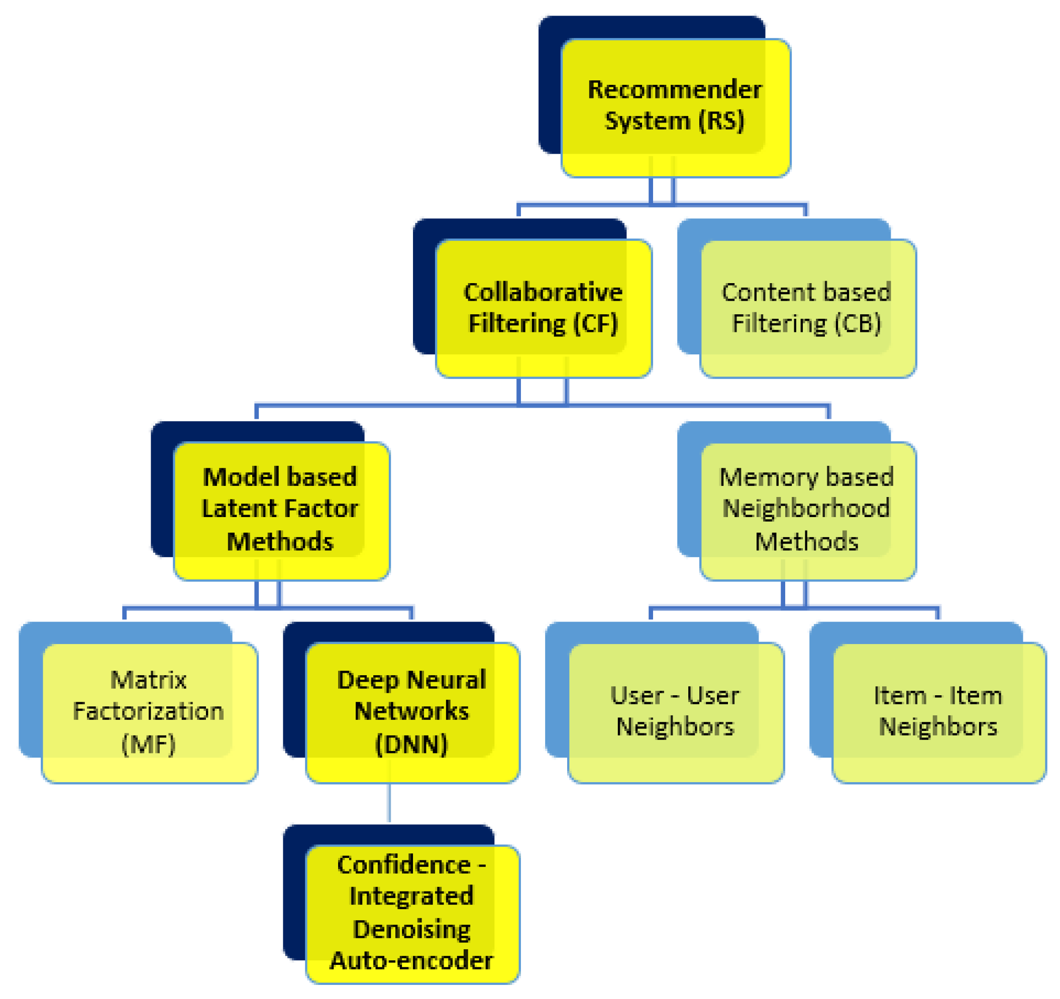
3. Auto-Encoder Variants for Recommender Systems

This section includes the description and update relations for the standard auto-encoder, denoising auto-encoder and the proposed confidence-aware denoising auto-encoder.

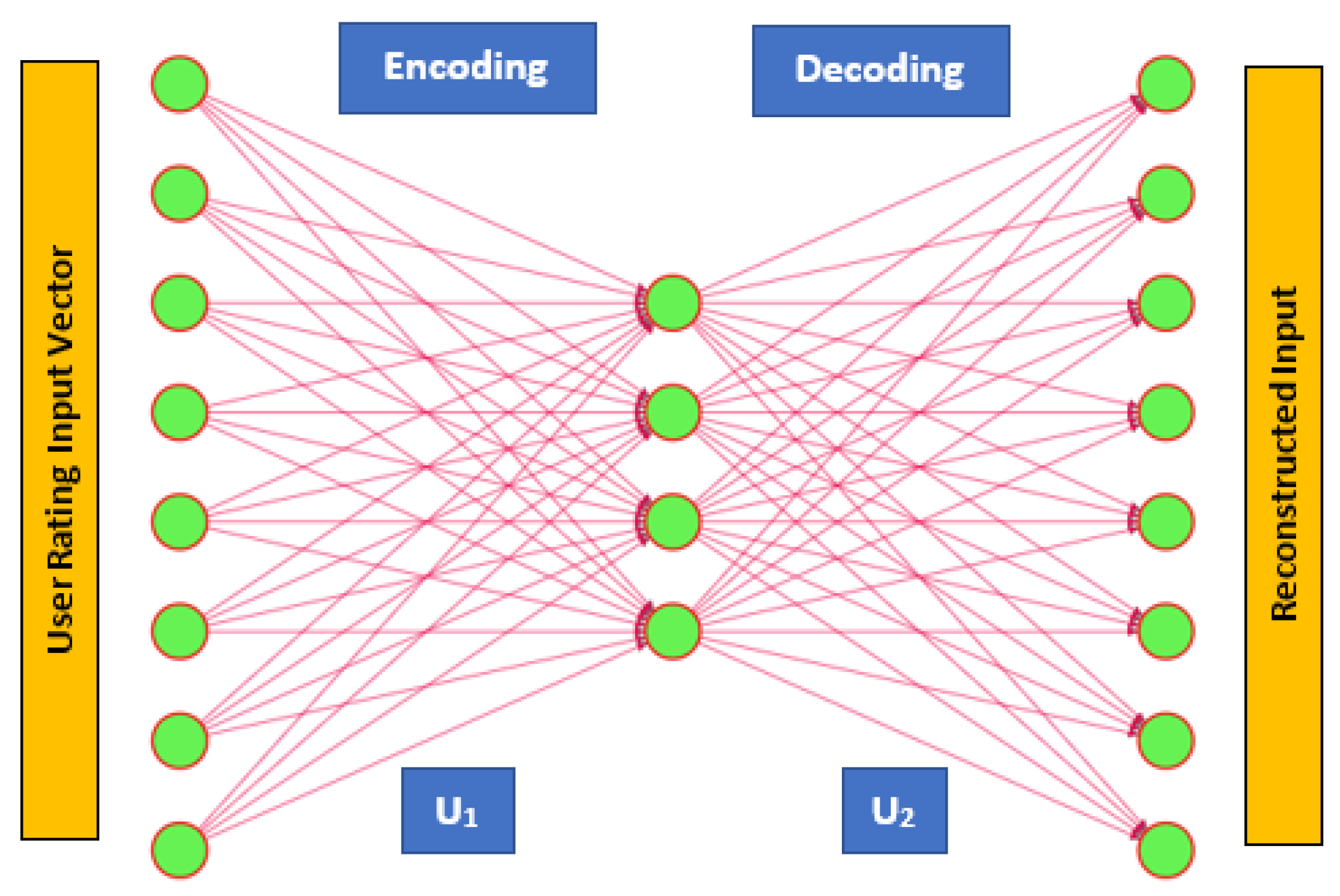
3.1. Auto-Encoder (AE)

The architecture of an AE [52] for an RS is made up of encoding and decoding parts. The encoding part includes an input layer and the hidden layer, which is used to extract significant latent representations from a sparse input vector, $x\in {ℝ}^k,$ of an input preference matrix, $R\in {ℝ}^{a\times b}$, to a space, $\left(S\right),$ with reduced dimensions. The decoding part consists of a hidden layer and the output layer. The role of the decoding part is to reconstruct the original input from the reduced latent representations, wherein $v_{\mathscr{H}}\in {ℝ}^S$, is the hidden layer’s bias and the matrix ${\mathrm{U}}_1\in {ℝ}^{k\times S}$ is the weight matrix of the input layer connected to the hidden layer. Likewise,$v_O\in {ℝ}^k$ signifies the output layer bias, and ${\mathrm{U}}_2\in {ℝ}^{S\times k}$ represents the weights associated with the output layer and the hidden layer. The multi-neural architecture of the standard AE is demonstrated in Figure 2.

To solve the reconstruction loss, parameters $\mathsf{\yen }=\{{\mathrm{U}}_1,{\mathrm{U}}_2,v_{\mathscr{H}},v_O\},$ including the weights and biases of the AE, are updated using a back-propagation algorithm. The cross-entropy loss is used for the binary inputs and the squared loss is used for regression. The cost function of a standard AE with $m$ users is represented as:

$$\underset{\mathsf{\yen }}{\min }\frac{1}{m}{\displaystyle \sum }_{u=1}^mℒ\left(x,\widehat{x}\right)+\Re \left({\mathrm{U}}_1, {\mathrm{U}}_2, v_{\mathscr{H}}, v_O\right)$$

(1)

The squared loss for the auto-encoder is represented as:

$$ℒ\left(x,\widehat{x}\right)=\Vert x_u-{\widehat{x}}_u\Vert {}_2^2$$

(2)

the cross-entropy loss for an auto-encoder is given as:

$$\begin{gathered} ℒ\left(x_u,{\widehat{x}}_u\right)=-x_u{}^T\log \left({\widehat{x}}_u\right) \\ -{\left(1-x_u\right)}^T\log \left(1-{\widehat{x}}_u\right) \end{gathered}$$

(3)

In order to obtain the reconstruction loss, back-propagation is employed to learn (train) the parameters $\mathsf{\yen }=\{{\mathrm{U}}_1,{\mathrm{U}}_2,v_{\mathscr{H}},v_O\}$ for the encoder. In the objective function, $\Re$ represents the regularization term with the squared norm (${\ell }_2$) of the parameters to be learned, presented as:

$$\begin{gathered} \Re \left({\mathrm{U}}_1, {\mathrm{U}}_2 , v_{\mathscr{H}}, v_O\right) \\ =\frac{\lambda }{2}(\Vert {\mathrm{U}}_1\Vert {}_2^2+\Vert {\mathrm{U}}_2\Vert {}_2^2+\Vert v_{\mathscr{H}}\Vert {}_2^2 \\ +\Vert v_O\Vert {}_2^2) \end{gathered}$$

(4)

The activation function activates and deactivates the neurons at the hidden layer and is represented by $\mathscr{H}$:

$$\mathscr{H}\left(x\right)=f\left({\mathrm{U}}_1^{\mathrm{T}}x+v_{\mathscr{H}}\right)$$

(5)

Different types of activation functions, $f\left(·\right),$ can be employed for the purpose of firing the neurons, such as relu, sigmoid, or identity [52]. For a sigmoid activation function, the hidden layer can be written as:

$$\mathscr{H}\left(x\right)=Sigmoid\left({\mathrm{U}}_1^{\mathrm{T}}x+v_{\mathscr{H}}\right)=\sigma \left({\mathrm{U}}_1^{\mathrm{T}}t+v_{\mathscr{H}}\right)$$

(6)

The input is recovered by applying the latent representations accumulated in the bottleneck layer (hidden layer) to the reconstruction layer (output layer). Finally, the Sigmoid activation function is again employed at the reconstruction layer. The recovered estimated vector input can be provided as:

$$\widehat{x}=g\left({\mathrm{U}}_2^{\mathrm{T}}\mathscr{H}\left(x\right)+v_O\right)$$

(7)

The final, estimated input vector via the Sigmoid is provided as:

$$\begin{gathered} \widehat{x}=Sigmoid\left({\mathrm{U}}_2^{\mathrm{T}}\mathscr{H}\left(x\right)+v_O\right) \\ =\sigma \left({\mathrm{U}}_2^{\mathrm{T}}\mathscr{H}\left(x\right)+v_O\right) \end{gathered}$$

(8)

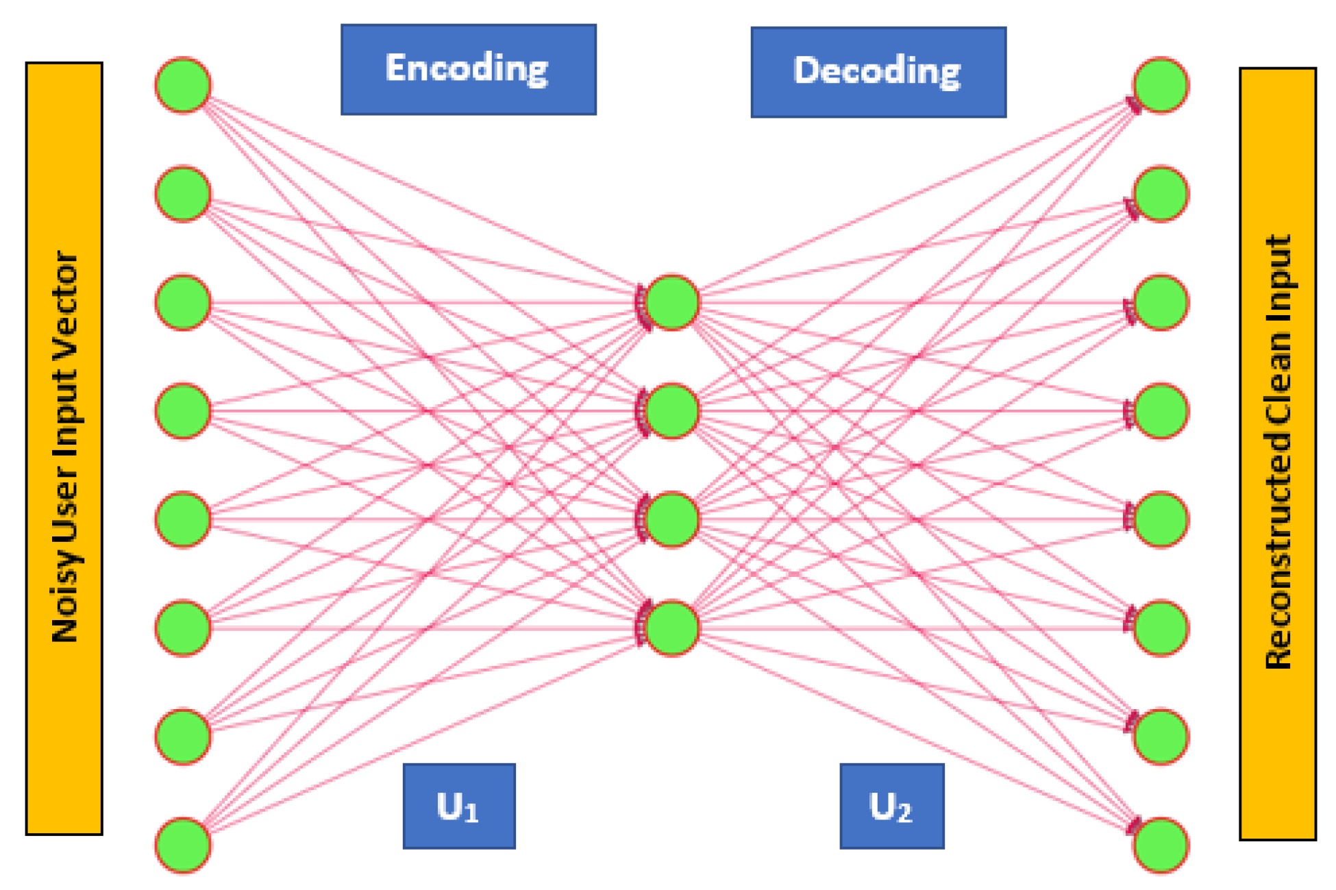
3.2. Denoising Auto-Encoder (DAE)

A DAE is another variation of a basic auto-encoder [63]. The input to a DAE is noisy data instead of clean data. A clean input, $x,$ is partially corrupted to $\overline{x}$ through stochastic mapping $\overline{x}\sim a(\overline{x}|x)$ [63]. The corruption in the input is drawn randomly from the conditional distribution, $p(\overline{x}|x)$. The input corruption options may include Gaussian noise, $p\left(\overline{x}|x\right)=\mathbb{N}\left(x,{\displaystyle \sum }\right)$ (where the co-variance matrix is independent of $x$), or mask-out-noise (where each input entry is randomly diffused by zero with $a$ probability), such as $P\left(\overline{x}=0\right)=a$ and $P\left(\overline{x}=1/\left(1-a\right)x\right)=1-a$. Mask-out corruption is used in this study for all denoising auto-encoder algorithms. A DAE is designed to recover the input from its corrupted form. DAEs are more robust than the basic auto-encoders due to their capability in handling noisy data [64]. A DAE with noisy inputs is graphically demonstrated in Figure 3.

3.3. Confidence-Integrated Denoising Auto-Encoder (CIDAE)

The confidence-aware DAE is designed by using the complete dataset instead of only positive feedback [51] from the users. The utilization of all the available ratings of the dataset provides us more information for better top-N recommendations by incorporating the negative ratings of the dataset. In a ranking-based evaluation, top-N ranking is a common approach to recommending a set of top-N-ranked items to the users. The benefit of modeling a rating trend for top-N recommendations is to recommend an unrated set of items to the user by approximating the dominating preference behavior (ratings) of a user for a rated set of items. In the top-N items ranking approach, a set of top-N-ranked items are selected from a sorted list of N items recommended to a user. A set of items that is recommended to the user is equal in size to the recommended list of top-N items.

We employed a cross-entropy loss function that involved the weights as the user’s preference value, and a user’s confidence value was assigned to feedback for specific items. The confidence-integrated loss of a DAE is represented as:

$$\begin{gathered} ℒ\left(x_u,{\widehat{x}}_u\right)=C{V}_{u,i}[-P{V}_{u,i}\log \left({\widehat{x}}_u\right) \\ -\left(1-P{V}_{u,i}\right)\log \left(1-{\widehat{x}}_u\right)] \end{gathered}$$

(9)

Here, $P{V}_{u,i}$ represents the preference function that returns a 1 for positive feedback and 0 for negative feedback, summarized as:

$$P{V}_{u,i}=\{\begin{array}{c}1, if x_{u,i}\ge 4\\ 0, otherwise\end{array}$$

(10)

whereas $C{V}_{u,i}$ shows the confidence function for feedback, provided as:

$$C{V}_{u,i}=\{\begin{array}{c}\beta , if x_{u,i}=1 or x_{u,i}=5 \hfill \\ 0.5\beta if x_{u,i}=2 or x_{u,i}=4 \hfill \\ 0.1\beta otherwise\hfill \end{array}$$

(11)

Here, $\beta$ is a hyper-parameter, and the optimal $\beta$ value is selected through a hyper-parameter-tuning mechanism. It can be seen that the ${CV}_{u,i}$ value reflects a higher confidence value for the minimum and maximum ratings and a lower confidence value for the intermediate ratings.

Using the Equations (4) and (9), the objective function for the proposed CIDAE is as follows:

$$\underset{\mathsf{\yen }}{\min }\frac{1}{a}{\displaystyle \sum }_{u=1}^{a}C{V}_{u,i}[-P{V}_{u,i}\log \left({\widehat{x}}_u\right)-\left(1-P{V}_{u,i}\right)\log \left(1-{\widehat{x}}_u\right)]+\frac{\lambda }{2}(\Vert {\mathrm{U}}_1\Vert {}_2^2+\Vert {\mathrm{U}}_2\Vert {}_2^2+\Vert v_{\mathscr{H}}\Vert {}_2^2+\Vert v_O\Vert {}_2^2)$$

(12)

The network architecture of the suggested CIDAE for top-N recommendations is presented in Figure 4.

The overall flow of the proposed CIDAE for proposing top-N recommendations is graphically shown in Figure 5. However, the step-by-step pseudo-code of the proposed CIDAE is provided in Algorithm 1.

Algorithm 1. Pseudocode of the suggested CIDAE method

Input: confidence‐aware, corrupted user‐preference vectors Output: clean user-preference vectors for top-N recommendations (1) Initialize parameters $\mathsf{\yen }=\{{\mathrm{U}}_1,{\mathrm{U}}_2,v_{\mathscr{H}},v_O\}$ randomly (2) Generate Confidence Values for Observed Ratings (3) Convert Numerical Feedback into Binary one (4) Add mask-out noise to partially corrupt input user vector ${\overline{x}}_u~p\left({\overline{x}}_u|x_u\right)$ (5) Set epoch = 1 (6) While $Iter<Iters$ do (7)     for all $u\in M$ do (8)      Calculate Objective Function using Equation (12) (9)      Compute P@10, NDCG@10, R@5, R@10, MAP via Equations (13)–(20) (10)      Take negative samples ${ℂ}_{mis}\subset {\overline{\wp }}_u$ (11)       for all $j\in {\wp }_u{\displaystyle \cup }{ℂ}_{mis}$ do (12)         Update parameters $\mathsf{\yen }=\{{\mathrm{U}}_1,{\mathrm{U}}_2,v_{\mathscr{H}},v_O\}$ (13)       end for (14)     end for (15)     $Iter=Iter+1$ (16) end while

4. Simulations and Results

This section includes subsections such as data manipulation, dataset particulars, a simulation description, simulation settings, ranking-based evaluation metrics, results and discussion, and a detailed analysis.

4.1. Data Manipulation

The input rating matrix was divided into training and test sets with test and train fractions of 80% and 20%, respectively. Initially, we found a confidence matrix using the complete set of observed training examples by assigning different confidence values for numerical ratings in the range of 1 to 5. Later, to represent the maximum and minimum ratings in terms of binary values, the explicit numerical ratings given in the range of 1 to 5 were converted into binary ratings (1 and 0).

4.2. Datasets Particulars

The efficiency of the proposed CIDAE with regard to precision and accuracy when compared to the standard counterparts was confirmed through two MovieLens [65] benchmark datasets, i.e., ML-1M and ML-100K. MovieLens datasets are extensively used as popular datasets for evaluating RSs through ranking-based metrics for top-N recommendations. Both datasets contain numerical feedback of 1 to 5 and the minimum ratings provided by a user in both datasets are at least 20. The statistics of both datasets are described in

Table 1. Statistics of datasets.

Dataset	Total Ratings (R)	Number of Users (U)	Number of Items (I)	Density (%) R/(U*I) * 100	Min (R/U)
ML-100K	100K	943	1682	6.30	20
ML-1M	1M	6040	3706	4.47	20

.

4.3. Simulation Description

A grid search was chosen as a hyper-parameters selection and tuning method, consuming training examples for the evaluation of all methods. We used a 5-fold cross-validation to choose the train and test sets randomly for 100 iterations. The average values of the findings are reported for all techniques. Methods were assessed for multiple learning rate values, i.e., [0.001, 0.005, 0.01, 0.05, 0.06, 0.08, and 0.1, 0.5], and the results for the optimum initial value of the learning rate for different methods are stated. Lambda ($\lambda$) is the regularization parameter for the penalty term involved in the objective function of the recommender systems. It is a common practice to use a smaller $\lambda$ value for regularizing the learned parameters (weights) to avoid overfitting on the observed ratings. From the deep analysis, it was noted that the small-value lambda, $\lambda$ = 0.01, in the baseline models (the CDAE and DAE) presented in [54] provided improved ranking-based predictions at the output layer. Likewise, we have considered the same value of $\lambda$ = 0.01 for the regularization of the penalty term.

Experiments were executed with a single hidden layer comprising 50 hidden nodes (latent dimensions) in the multi-neural architecture of all methods. An Adam optimizer was used for the weight update mechanism of all methods, with a mini batch size of 400 used for the ML-1M dataset and a mini batch size of 100 used for ML-100K dataset. Moreover, Adam automatically adapts the learning rate for the weight update expressions. Beta was another hyper-parameter empirically chosen such that $\beta <1$. It is inferred from the $\beta$ tuning that the performance of the proposed CIDAE began degrading at $\beta >0.1$, whereas the performance for some of the ranking-based evaluation measures improved slightly for $\beta <0.1$. Overall, the proposed CIDAE exhibited comparable performance for beta values of $\beta \le 0.1$. However, the CIDAE showed a stable and improved performance when compared to the CDAE and DAE with respect to the ranking evaluation metrics for a beta value of $\beta =0.1$.

The user input vectors were corrupted through masking noise ($N$), and the methods were evaluated via different ranking-based evaluation measures for two values of masking noise ($N$), i.e., [0.2, 0.5]. The masking noise variations represented the percentage of noise used (where the users’ input ratings are masked via zero considering the given noise ratio) to corrupt the input. For example, $N$ = 0.2 represented that 20 % of the users’ inputs were corrupted (overwritten) randomly through zero. A summary indicating the optimal values of the hyper-parameters used by the three methods is provided in

Table 2. Parameters for simulation.

Hyper-Parameters Used	Notation	Tested Hyper-Parameter Values	Values Chosen for CIDAE	Values Chosen for DAE	Values Chosen for CDAE
Latent Features	$K$	50	50	50	50
Learning Rate	$\mu$	0.001, 0.005, 0.01, 0.05, 0.06, 0.07, 0.08, 0.1, 0.5	0.06	0.01	0.01
Noise	$N$	0.2, 0.5, 0.8, 0.10	0.2, 0.5	0.2, 0.5	0.2, 0.5
Regularization Rate	$\lambda$	0.01	0.01	0.01	0.01
Confidence Value	$\beta$	0.1	0.1	0.1	0.1

.

4.4. Simulation Settings

All experiments were accomplished on a laptop with a Core-i7-5600U-@-2.6 Giga Hertz processor, 64-bit operating system, and 16 GB RAM. HP EliteBook 840 G2 Core-i7-5600U, 2.6 Giga Hertz processor, 64-bit operating system, and 16 GB RAM The algorithms were implemented in Python using TensorFlow.

4.5. Ranking-Based Evaluation Metrics

In a ranking-based evaluation, top-N ranking is a common approach to recommending a set of top-N-ranked items to users. An item set in top-N ranking is represented by $\text{£}\left(N\right)$. Let $T$ denote the set of all relevant items for a single user. Ranking-based top-N evaluation measures are mathematically represented as follows [1]:

Precision@N:

$$P@N=\left|\frac{\text{£}\left(K\right){\displaystyle \cap }\mathrm{T}}{\left|\text{£}\left(N\right)\right|}\right|\times 100$$

(13)

Recall@N:

$$R@N=\left|\frac{\text{£}\left(N\right){\displaystyle \cap }\mathrm{T}}{\left|\mathrm{T}\right|}\right|\times 100$$

(14)

Mean Average Precision:

$$MAP=\frac{1}{M}{\displaystyle \sum }_{u=1}^M{\left(AP@Hits\right)}_u$$

(15)

AP represents the average-precision of the relevant items of a user, $u,$ out of all hits of a recommendation set.

$$AP@Hits=\frac{1}{\mathrm{T}}{\displaystyle \sum }_{t=1}^{Hits}P\left(t\right).\Re \left(n\right)$$

(16)

Here, $\Re \left(n\right)$ specifies the relevance of $n^{th}$ item is false, $\left(\Re \left(n\right)=0\right),$ or true, $\left(\Re \left(n\right)=1\right)$.

Normalized Discounted Gain:

$$NDCG=\frac{DCG}{IDCG}$$

(17)

$$DCG=\frac{1}{M}{\displaystyle \sum }_{u=1}^M{\displaystyle \sum }_{iϵ{\mathbb{N}}_u}\frac{{\mho }_{ui}}{{\log }_2\left({ℝ}_i+1\right)}$$

(18)

Here, ${\mathbb{N}}_u$ denotes the item set rated by a user, $u,$ hidden from a recommender system before valuation and ${\Re }_{ui}$ shows the relevance of an item, $i$, for a user, $u$. ${\mho }_{ui}$ represents the utility of the $u$ user for the $i$ item, while ${ℝ}_i$ denotes rank of an item, $i,$ in a test set, ${\mathbb{N}}_u$.

$${\mho }_{ui}=2^{{\Re }_{ui}}-1$$

(19)

Here, ${\Re }_{ui}$ is the relevance of item $i$ for a user $u$.

Normalized Discounted Gain @N:

The discounted gain (DCG) can also be computed for a recommendation set of length $\mathsf{\Psi }\left(N\right),$ specified as:

$$DCG=\frac{1}{M}{\displaystyle \sum }_{u=1}^M{\displaystyle \sum }_{iϵ{\mathbb{N}}_u,w_i\le \mathsf{\Psi }\left(N\right)}\frac{{\mho }_{ui}}{{\log }_2\left({ℝ}_i+1\right)}$$

(20)

4.6. Results and Discussion

This section includes the comparative description and demonstration of the improved performance achieved by the proposed CIDAE over its counterparts, i.e., the DAE and CDAE, through ranking-based evaluation indices such as P@10, NDCG@10, R@5, R@10, MAP, and NDCG for two benchmark datasets of ML-100K and ML-1M. For a fair comparison, the results with respect to the evaluation measures are presented through tables, learning curves, and bar charts.

4.6.1. Explanation with Respect to the ML-100K Dataset

The performance outcomes of the three strategies with two noise variations, i.e., [0.2, 0.5] for ranking-based metrics using the ML-100K dataset are represented in

Table 3. Performance evaluation for noise variations using ML-100K.

Metric	$\mathit{N}$ = 0.2			$\mathit{N}$ = 0.5
	CIDAE	CDAE	DAE	CIDAE	CDAE	DAE
P@10	0.1839	0.1809	0.1807	0.1987	0.1945	0.1911
R@10	0.2125	0.1955	0.1950	0.2239	0.2177	0.2058
R@5	0.1335	0.1247	0.1223	0.1425	0.1384	0.1324
MAP	0.1841	0.1763	0.1732	0.2006	0.1939	0.1878
NDCG	0.4911	0.4842	0.4799	0.5087	0.4999	0.4952
NDCG@10	0.2519	0.2497	0.2460	0.2741	0.2693	0.2618

and Figure 6, Figure 7, Figure 8 and Figure 9. The proposed CIDAE demonstrated significant performance over the DAE and CDAE with both noise variations, i.e., [0.2, 0.5], for all ranking-based metrics stated in Table 3.

Initially, the performance of the proposed CIDAE was assessed via MAP and NDCG, and the numerical outcomes are listed in Table 3. The performance-based learning curves representing the MAP and NDCG for two noise variations are shown in Figure 6. It can be seen from the learning curves in Figure 6a–d that the CIDAE showed a substantial improvement in performance over the DAE and CDAE for all epochs and with both noise variations. The improvement in the performance of the CIDAE is the result of confidence values introduced in the cross-entropy objective function for the observed users’ feedback.

The results with respect to (R@5 and R@10) are also presented in Table 3, while the fitness curves depicting (R@5 and R@10) for different noise values, i.e., [0.2, 0.5], are given in Figure 7. It can be seen from the learning plots given in Figure 7a–d that the proposed CIDAE outperformed the DAE and CDAE for different noise values representing corruption in the users’ rating vectors. It can also be seen that the CIDAE achieved the fitness, i.e., (R@5 and R@10), in a smaller number of iterations when compared to the fitness achieved by its counterparts after 100 iterations. Moreover, it can be observed that the CIDAE also attained a better steady-state performance in terms of (R@5 and R@10) after 100 iterations. The reason for such an increase in performance is the exploitation of all observed ratings with respect to the confidence values assigned to the ratings set for the ML-100K dataset.

The performance of the proposed CIDAE is verified further through two more top-N-ranking metrics, P@10 and NDCG@10. The scores for precision and the normalized discounted gain are presented in Table 3. The P@10 and NDCG@10 curves for the assessment of the algorithms with two noise variants are demonstrated in Figure 8. From the learning curves given in Figure 8a–d, it is noted that the relative increase in performance of the proposed CIDAE for epochs greater than 10 is significantly better than the other two auto-encoder-based denoising variants for input corruption variations ($N$). Furthermore, the proposed CIDAE succeeded in attaining the comparative performance regarding P@10 and NDCG@10 in earlier iterations when compared to its counterparts. The CIDAE attained such an enhanced, accurate, and speedy performance due to the presence of a confidence-integrated, weighted-objective function, which was developed to associate the actual ratings (low or high) with a certain confidence value.

Figure 9 represents the bar graphs expressing the relative evaluation of the proposed CIDAE with the two rival methods, i.e., the DAE and CDAE, in terms of the steady-state performance for two noise variations consuming the ML-100K dataset.

Figure 9a represents the recall (R@5) scores after 100 epochs for the three methods, i.e., the DAE, CDAE, and the proposed CIDAE with two noise levels, i.e., [0.2, 0.5]. It is noted that CIDAE achieved substantial recall scores of (R@5 = 0.1335) and (R@5 = 0.1425) for both $N$ = 0.2 and $N$ = 0.5, respectively. The recall (R@10) scores for the DAE, CDAE, and CIDAE are shown in Figure 9b via bar-graphs with two input corruption-levels. It can be seen that for two values of noise, i.e., $N$ = 0.2 and $N$ = 0.5, CIDAE demonstrated a significant increase in recall scores of (R@10 = 0.2125) and (R@10 = 0.2239), respectively, when compared to the DAE and CDAE.

The steady-state performance of the three approaches, i.e., the DAE, CDAE, CIDAE, in terms of the (P@10) and (NDCG@10) scores for two noise levels are displayed in Figure 9c,d, respectively. A slight increase in the performance of the CIDAE (0.1839) with respect to a P@10 score for $N$ = 0.2 is observed when compared to the CDAE (0.1809) and DAE (0.1807) scores. A similar performance trend for the CIDAE (0.1987) is observed for P@10 with $N$ = 0.5, compared with the CDAE (0.1945) and DAE (0.1911). In contrast to the slight improvement regarding the P@10 scores, the CIDAE accomplished a significant rise in performance with respect to the NDCG@10 scores when compared to the CDAE and DAE for both noise levels. The maximum NDCG@10 scores reached by the CIDAE for $N$ = 0.2 and $N$ = 0.5 were (0.2519) and (0.2741), respectively.

Bar graphs representing the steady-state performance of the proposed CIDAE along with its counterparts in terms of the MAP and NDCG scores for two noise values after 100 iterations are demonstrated in Figure 9e,f, respectively. A considerable improvement in the steady-state performance of the CIDAE (0.1841) in comparison with the CDAE (0.1763) and the DAE (0.1732) with respect to the MAP score is observed for N = 0.2. For N = 0.5, CIDAE also attained a huge increase in performance with a MAP score of (0.2006), compared to the MAP scores achieved by the CDAE (0.1939) and DAE (0.1878). Similarly, a superior performance of CIDAE with respect to the NDCG scores is noted for $N$ = 0.2 and $N$ = 0.5 versus contending methods. The proposed CIDAE achieved NDCG scores of (0.4911) and (0.5087) for $N$ = 0.2 and $N$ = 0.5, respectively.

4.6.2. Explanation with Respect to the ML-1M Dataset

To authenticate the performance of the proposed CIDAE with respect to ranking-based valuation metrics over the DAE and CDAE, simulations were also performed using a larger dataset, i.e., ML-1M, for two noise levels, i.e., [0.2, 0.5]. The results for the ranking-based metrics are provided in

Table 4. Performance assessment for noise variations using ML-1M.

Metrics	$\mathit{N}$ = 0.2			$\mathit{N}$ = 0.5
	CIDAE	CDAE	DAE	CIDAE	CDAE	DAE
P@10	0.2011	0.2048	0.1993	0.2056	0.2162	0.1960
R@10	0.1589	0.1441	0.1400	0.1608	0.1583	0.1338
R@5	0.1004	0.0904	0.0880	0.0999	0.1000	0.0837
MAP	0.1632	0.1539	0.1504	0.1629	0.1679	0.1457
NDCG	0.5001	0.4876	0.4826	0.5001	0.5042	0.4771
NDCG@10	0.2498	0.2507	0.2442	0.2574	0.2670	0.2388

and are demonstrated in Figure 10, Figure 11, Figure 12 and Figure 13.

Figure 10 exhibits the learning curves for R@5 and R@10 for two noise variations, i.e., [0.2, 0.5]. The learning plots presented in Figure 10a–d show that the proposed CIDAE performed substantially better for all epochs with two noise variations. It can also be seen that the recall scores achieved by the DAE and CDAE after 100 iterations were achieved by CIDAE earlier, after consuming 40 iterations. Moreover, the final recall score achieved by the CIDAE was also higher when compared to the DAE and CDAE. The CIDAE attained such recommendation speed due to the confidence-integrated design of the CIDAE for top-N recommendations.

The learning plots representing the relative performance of the three methods, i.e., DAE, CDAE, and the proposed CIDAE, in terms of the MAP and NDCG with two noise values are given Figure 11. It is noted from Figure 11a,b that the CIDAE achieved considerable progress in performance when compared to its rival methods for noise value ($N$ = 0.2) with respect to the MAP and NDCG scores for 100 iterations. Additionally, the CIDAE attained the MAP and NDCG scores far earlier, i.e., at 50 iterations, when compared to the scores achieved by the DAE and CDAE after 100 iterations. Furthermore, it is seen from Figure 11c,d that, for $N$ = 0.5, there was a marked rise in the performance of the CIDAE for the MAP and NDCG over the CDAE until 75 iterations, but that CIDAE demonstrated a comparable performance afterwards.

However, for $N$ = 0.5, the CIDAE outperformed the DAE with regard to the MAP and NDCG scores for almost all iterations, as is shown in Figure 11c,d. The improved and competitive performance of the CIDAE over its counterparts is the outcome of the mapping between the users’ feedback and the confidence values assigned to that feedback.

The relative performance of the proposed CIDAE over the DAE and CDAE is also validated for two more ranking-based evaluation metrics, i.e., P@10 and NDCG@10, for top-N recommendations. The comparative results for two noise variations are represented through learning curves in Figure 12. It can be observed from the plots given in Figure 12a,b that for $N$ = 0.2, the performance of the proposed CIDAE with respect to P@10 and NDCG@10 over the DAE was noticeably raised for 100 iterations, whereas the CIDAE achieved a great improvement in performance in terms of P@10 and NDCG@10 when compared to the CDAE for 90 epochs and achieved similar results for P@10 and NDCG@10 after 90 epochs. In addition, it can be observed from Figure 12c,d that the CIDAE increased from the 5th to 70th iterations.

The CIDAE attained a superior performance for P@10 and NDCG@10 over the CDAE for $N$ = 0.5 and demonstrated a slightly reduced performance trend for subsequent iterations. However, the CIDAE demonstrated a remarkable performance (P@10 and NDCG@10) for $N$ = 0.5 when compared to the DAE for all iterations.

To prove the scalability of the proposed CIDAE over its counterparts, the comparative assessment of the proposed CIDAE with the CDAE and DAE was also performed for a bigger MovieLens dataset i.e., ML-1M. The results of the ranking-based evaluation metrics representing steady-state performance after 100 iterations with two noise variations are presented in Figure 13.

The results in terms of the (R@5) score achieved by the CIDAE, CDAE and DAE after 100 epochs and with two noise values, i.e., [0.2, 0.5], are provided in Figure 13a. The CIDAE achieved a significantly improved R@5 score (0.1004) for $N$ = 0.2 over the CDAE (0.0904) and DAE (0.0880). The score attained by the CIDAE (0.0999) for $N$ = 0.5 was also substantial over DAE (0.0837), but the CIDAE slightly lagged behind the CDAE (0.1000). The bar graphs for (R@10) for the three methods with distinct noise values are presented in Figure 13b. The proposed CIDAE leads the CDAE and DAE in terms of the R@10 scores for both noise variations. The R@10 values attained by the CIDAE for $N$ = 0.2 and 0.5 are 0.1589 and 0.1608, respectively.

The bar graphs shown in Figure 13c exhibit (P@10) scores for the denoising auto-encoder variants with different noise levels, i.e., [0.2, 0.5]. It is noted from Figure 13c that the performance of the CIDAE was improved drastically over the DAE for $N$ = 0.2, whereas comparable results with respect to P@10 can be observed for both the CIDAE and CDAE, with $N$ = 0.5. Figure 13d demonstrates the NDCG@10 scores for the contending methods, given two noise variations. There was a slight increase in the NDCG@10 score gained by the CIDAE over the DAE, with $N$ = 0.2. However, the performance (NDCG@10) of the CIDAE when compared to the CDAE was decreased marginally for $N$ = 0.5.

The steady-state performance of the CDAE over three models was also evaluated for the MAP score with two noise levels. It is presented in Figure 13e. For $N$ = 0.2, the CIDAE accomplished a noticeably improved MAP score (0.1632) after 100 iterations when compared to the CDAE (0.1539) and DAE (0.1504). In contrast to $N$ = 0.2, the CIDAE did not succeed in achieving a superior MAP score for $N$ = 0.5 when compared to the CDAE. Therefore, the performance of both methods for $N$ = 0.5 was comparable. Additionally, the bar graphs representing the NDCG score for the two noise variations are shown in Figure 13f. It can be perceived from Figure 13f that the NDCG performance trend, in terms of NDCG demonstrated by the CIDAE over the CDAE and DAE, with two noise values was similar to that of the performance achieved by the CIDAE with respect to the MAP.

4.7. Critical Observations

The in-depth investigation of the study is as follows:

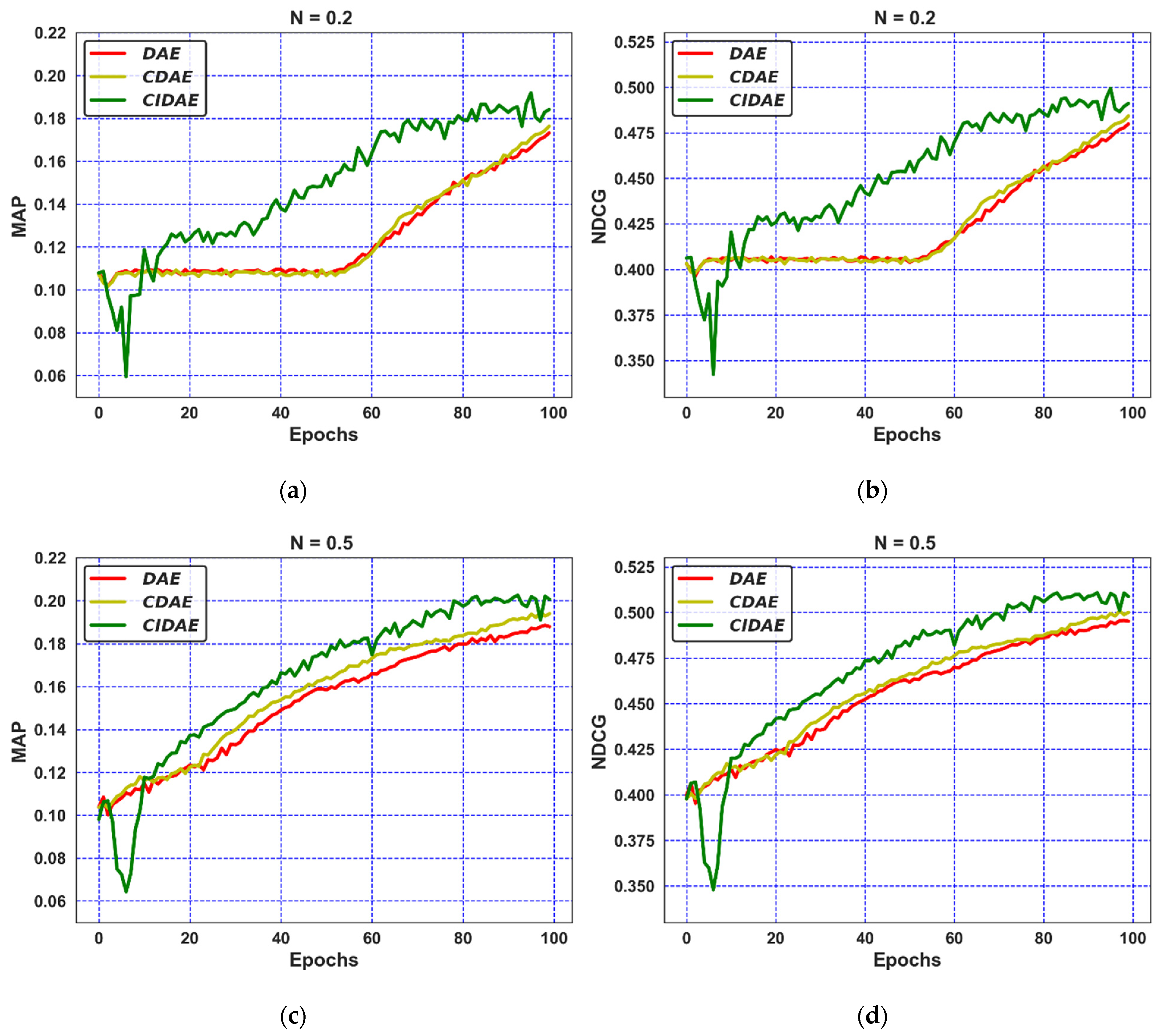
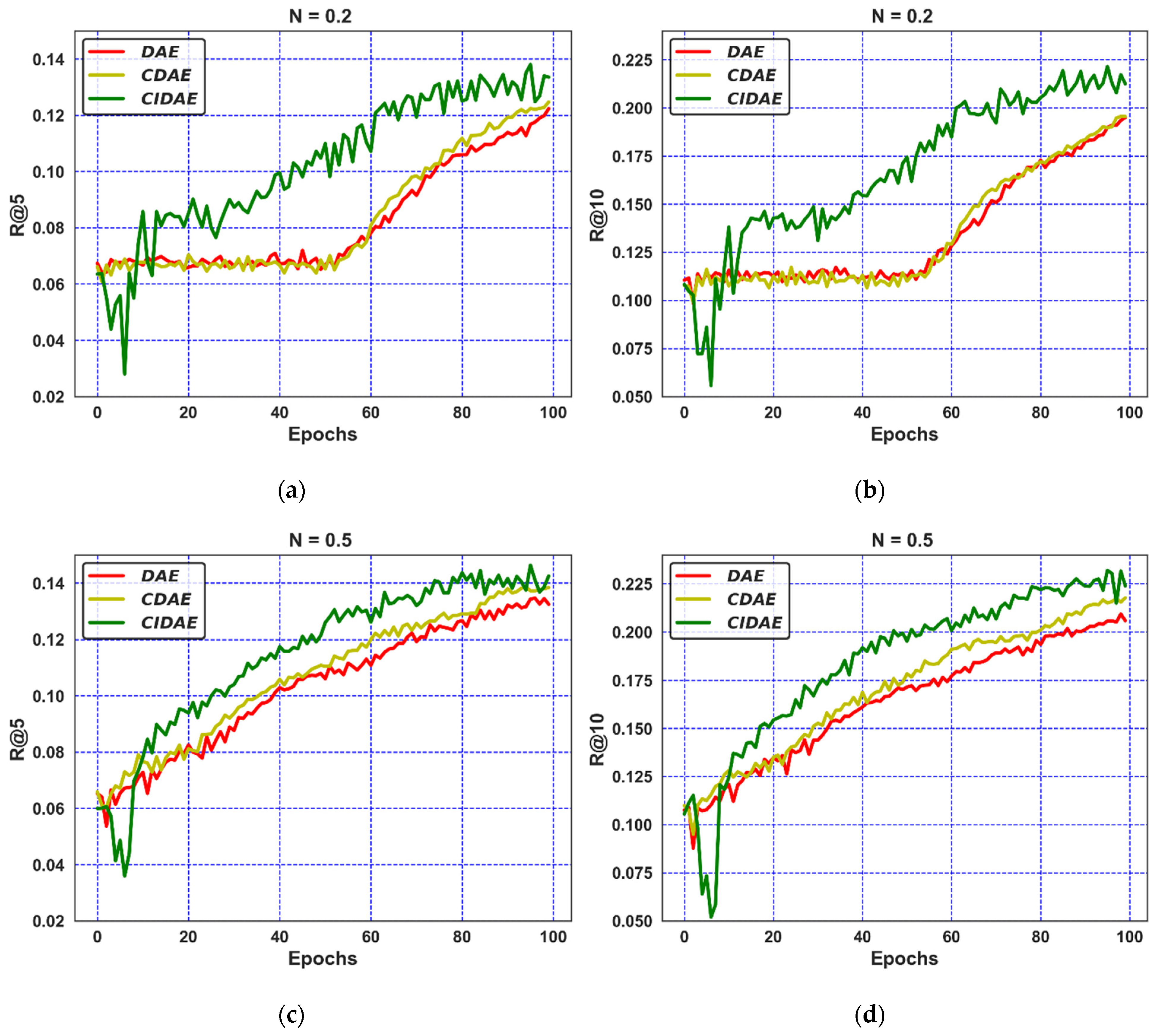
• The performance attained by the proposed CIDAE in fewer iterations for both noise variations indicates the improved speed for providing the top-N recommendations;
• The better steady-state performance, regardless of changes in noise levels, confirms the robustness and accuracy of the proposed CIDAE over its counterparts;
• The improved performance of the proposed CIDAE for both datasets verifies the scalability of the model when compared to the DAE and CDAE;
• A noticeable increase in performance in terms of all ranking-based measures is observed with $N$ = 0.5 compared to $N$ = 0.2 for the proposed CIDAE, which confirms that the CIDAE has the ability to perform better for more randomly overwritten zero values with the probability of $N$ = 0.5;
• The relative progress in the performance of the proposed CIDAE for iterations greater than 10 is considerably improved when compared to the two contending auto-encoder-based denoising techniques for noise variations ($N$);
• The CIDAE attains its enhanced, accurate, and speedy performance due to the presence of a confidence-integrated, weighted-objective function which associates the actual ratings (low or high) to a certain confidence value.

4.8. Implications

• Assigning the confidence values to the ratings highlights the importance of an explicit feedback (either high or low) given by a user with a particular state of mind;
• The prediction of missing feedback using higher (positive) and lower (negative) ratings;
• The proposed model provides an opportunity to utilize a full set of observed ratings rather than preferential ratings (positive-only feedback) to exploit the full information hidden in low, intermediate, and high ratings;
• The proposed confidence-aware strategy contributes as a significant addition to the e-commerce industry for increasing the potential of DAE-based recommendation models in term of the speed and accuracy of the recommendations.

5. Conclusions

The conclusions drawn from the study are stated as follows:

• We have suggested a confidence-aware denoising auto-encoder model (CIDAE) that exploits a complete set of observed ratings for an enhanced accuracy in providing top-N recommendations to users. The proposed CIDAE showed significantly improved results in terms of the recommendation speed over two denoising auto-encoder variants (DAE and CDAE) for smaller noise values, i.e., $N$ = 0.2. This is because a smaller noise value supports the maintenance of a noticeable proportion of users’ confidence with respect to the observed ratings in the dataset, providing useful information to the CIDAE for modeling confidence-aware top-N recommendations correctly;
• The comparison of the developed strategy (CIDAE) with state-of-the-art denoising auto-encoders (DAE and CDAE) with respect to standard, ranking-based evaluation metrics indicates a relatively improved performance of the CIDAE for suggesting top-N recommendations to the candidate users;
• The proposed CIDAE achieved a substantial steady-state performance for both noise levels with the ML-100K dataset, whereas the CIDAE attained improved results on the ML-1M dataset for a low noise level ($N$ = 0.2) and comparable results for a high noise level ($N$ = 0.5). Such behavior confirms the robustness and scalability of the proposed CIDAE over its counterparts.

Future research may consider investigating the application of the proposed methodology for solving MEMS problems [60,61,62,63,64,65].

References

1. Aggarwal, C.C. An Introduction to Recommender Systems. In Recommender Systems; Springer International Publishing: Cham, Switzerland, 2016; pp. 1–28. [Google Scholar]
2. Bobadilla, J.; Ortega, F.; Hernando, A.; Gutiérrez, A. Recommender systems survey. Knowl.-Based Syst. 2013, 46, 109–132. [Google Scholar] [CrossRef]
3. Konstan, J.A. Introduction to recommender systems. In Proceedings of the ACM SIGMOD International Conference on Management of Data; Springer US: Boston, MA, USA, 2008; p. 1373, ISBN 9781605581026. [Google Scholar]
4. Jayalakshmi, S.; Ganesh, N.; Čep, R.; Senthil Murugan, J. Movie Recommender Systems: Concepts, Methods, Challenges, and Future Directions. Sensors 2022, 22, 4904. [Google Scholar] [CrossRef]
5. Heimbach, I.; Gottschlich, J.; Hinz, O. The value of user’s Facebook profile data for product recommendation generation. Electron. Mark. 2015, 25, 125–138. [Google Scholar] [CrossRef]
6. Salau, L.; Hamada, M.; Prasad, R.; Hassan, M.; Mahendran, A.; Watanobe, Y. State-of-the-Art Survey on Deep Learning-Based Recommender Systems for E-Learning. Appl. Sci. 2022, 12, 11996. [Google Scholar] [CrossRef]
7. Alhijawi, B.; Kilani, Y. The recommender system: A survey. Int. J. Adv. Intell. Paradig. 2020, 15, 229. [Google Scholar] [CrossRef]
8. Venkatesan, R. Sabari A Issues in various recommender system in e-commerce—A survey. J. Crit. Rev. 2020, 7, 604–608. [Google Scholar]
9. Karimi, M.; Jannach, D.; Jugovac, M. News recommender systems—Survey and roads ahead. Inf. Process. Manag. 2018, 54, 1203–1227. [Google Scholar] [CrossRef]
10. Eirinaki, M.; Gao, J.; Varlamis, I.; Tserpes, K. Recommender Systems for Large-Scale Social Networks: A review of challenges and solutions. Future Gener. Comput. Syst. 2018, 78, 413–418. [Google Scholar] [CrossRef]
11. Amato, F.; Moscato, V.; Picariello, A.; Piccialli, F. SOS: A multimedia recommender System for Online Social networks. Future Gener. Comput. Syst. 2019, 93, 914–923. [Google Scholar] [CrossRef]
12. Chamoso, P.; Rivas, A.; Rodríguez, S.; Bajo, J. Relationship recommender system in a business and employment-oriented social network. Inf. Sci. 2018, 433–434, 204–220. [Google Scholar] [CrossRef]
13. Xiong, P.; Zhang, L.; Zhu, T.; Li, G.; Zhou, W. Private collaborative filtering under untrusted recommender server. Future Gener. Comput. Syst. 2020, 109, 511–520. [Google Scholar] [CrossRef]
14. Kaur, H.; Kumar, N.; Batra, S. An efficient multi-party scheme for privacy preserving collaborative filtering for healthcare recommender system. Future Gener. Comput. Syst. 2018, 86, 297–307. [Google Scholar] [CrossRef]
15. Hong, M.; Jung, J.J. Multi-Sided recommendation based on social tensor factorization. Inf. Sci. 2018, 447, 140–156. [Google Scholar] [CrossRef]
16. Yu, W.; Li, S. Recommender systems based on multiple social networks correlation. Future Gener. Comput. Syst. 2018, 87, 312–327. [Google Scholar] [CrossRef]
17. Meng, S.; Qi, L.; Li, Q.; Lin, W.; Xu, X.; Wan, S. Privacy-preserving and sparsity-aware location-based prediction method for collaborative recommender systems. Futur. Gener. Comput. Syst. 2019, 96, 324–335. [Google Scholar] [CrossRef]
18. Cui, C.; Qin, J.; Ren, Q. Deep Collaborative Recommendation Algorithm Based on Attention Mechanism. Appl. Sci. 2022, 12, 10594. [Google Scholar] [CrossRef]
19. Salter, J.; Antonopoulos, N. CinemaScreen Recommender Agent: Combining Collaborative and Content-Based Filtering. IEEE Intell. Syst. 2006, 21, 35–41. [Google Scholar] [CrossRef]
20. Mobasher, B. Data Mining for Web Personalization. In The Adaptive Web; Springer: Berlin/Heidelberg, Germany, 2007; Volume 4321 LNCS, pp. 90–135. ISBN 3540720782. [Google Scholar]
21. Aslanian, E.; Radmanesh, M.; Jalili, M. Hybrid Recommender Systems based on Content Feature Relationship. IEEE Trans. Ind. Inform. 2016, 1. [Google Scholar] [CrossRef]
22. Peng, D.; Yuan, W.; Liu, C. HARSAM: A Hybrid Model for Recommendation Supported by Self-Attention Mechanism. IEEE Access 2019, 7, 12620–12629. [Google Scholar] [CrossRef]
23. Köhler, S.; Wöhner, T.; Peters, R. The impact of consumer preferences on the accuracy of collaborative filtering recommender systems. Electron. Mark. 2016, 26, 369–379. [Google Scholar] [CrossRef]
24. He, C.; Parra, D.; Verbert, K. Interactive recommender systems: A survey of the state of the art and future research challenges and opportunities. Expert Syst. Appl. 2016, 56, 9–27. [Google Scholar] [CrossRef]
25. Chen, R.; Hua, Q.; Chang, Y.S.; Wang, B.; Zhang, L.; Kong, X. A survey of collaborative filtering-based recommender systems: From traditional methods to hybrid methods based on social networks. IEEE Access 2018, 6, 64301–64320. [Google Scholar] [CrossRef]
26. Cunha, T.; Soares, C.; de Carvalho, A.C.P.L.F. Metalearning and Recommender Systems: A literature review and empirical study on the algorithm selection problem for Collaborative Filtering. Inf. Sci. 2018, 423, 128–144. [Google Scholar] [CrossRef]
27. Li, J.; Zhang, K.; Yang, X.; Wei, P.; Wang, J.; Mitra, K.; Ranjan, R. Category Preferred Canopy–K-means based Collaborative Filtering algorithm. Futur. Gener. Comput. Syst. 2019, 93, 1046–1054. [Google Scholar] [CrossRef]
28. Hayakawa, M. MF Techniques. In Earthquake Prediction with Radio Techniques; Wiley: Hoboken, NJ, USA, 2015; pp. 199–207. [Google Scholar] [CrossRef]
29. Colace, F.; Conte, D.; De Santo, M.; Lombardi, M.; Santaniello, D.; Valentino, C. A content-based recommendation approach based on singular value decomposition. Conn. Sci. 2022, 34, 2158–2176. [Google Scholar] [CrossRef]
30. Ben Schafer, J.; Konstan, J.A.; Riedl, J. E-commerce recommendation applications. Data Min. Knowl. Discov. 2001, 5, 115–153. [Google Scholar] [CrossRef]
31. Wang, J.; de Vries, A.P.; Reinders, M.J.T. On Combining User-based and Item-based Collaborative Filtering. In Proceedings of the Twenty-Seventh Symposium on Information Theory in the Benelux, Noordwijk, The Netherlands, 8–9 June 2006; 2006; pp. 307–315. [Google Scholar]
32. Hernández-Lobato, J.M.; Houlsby, N.; Ghahramani, Z. Probabilistic matrix factorization with non-random missing data. In Proceedings of the International Conference on Machine Learning 2014, Beijing, China, 21–26 June 2014; 2014; Volume 4, pp. 3394–3436. [Google Scholar]
33. Wang, S.; Tang, J.; Wang, Y.; Liu, H. Exploring hierarchical structures for recommender systems. IEEE Trans. Knowl. Data Eng. 2018, 30, 1022–1035. [Google Scholar] [CrossRef]
34. Ning, X.; Desrosiers, C.; Karypis, G. A Comprehensive Survey of Neighborhood-Based Recommendation Methods. In Recommender Systems Handbook; Springer US: Boston, MA, USA, 2015; pp. 37–76. ISBN 9781489976376. [Google Scholar]
35. Pan, Y.; He, F.; Yu, H. A novel Enhanced Collaborative Autoencoder with knowledge distillation for top-N recommender systems. Neurocomputing 2019, 332, 137–148. [Google Scholar] [CrossRef]
36. Park, M.-H.; Hong, J.-H.; Cho, S.-B. Location-Based Recommendation System Using Bayesian User’s Preference Model in Mobile Devices. In Ubiquitous Intelligence and Computing; Springer: Berlin/Heidelberg, Germany, 2007; pp. 1130–1139. [Google Scholar]
37. Linqi, G.; Congdong, L. Hybrid personalized recommended model based on genetic algorithm. In Proceedings of the 2008 4th International Conference on Wireless Communications, Networking and Mobile Computing, Dalian, China, 12–14 October 2008; pp. 1–4. [Google Scholar] [CrossRef]
38. Luo, X.; Xia, Y.; Zhu, Q. Incremental Collaborative Filtering recommender based on Regularized Matrix Factorization. Knowl.-Based Syst. 2012, 27, 271–280. [Google Scholar] [CrossRef]
39. Casillo, M.; Gupta, B.B.; Lombardi, M.; Lorusso, A.; Santaniello, D.; Valentino, C. Context Aware Recommender Systems: A Novel Approach Based on Matrix Factorization and Contextual Bias. Electronics 2022, 11, 1003. [Google Scholar] [CrossRef]
40. Bokde, D.; Girase, S.; Mukhopadhyay, D. Matrix Factorization Model in Collaborative Filtering Algorithms: A Survey. Procedia Comput. Sci. 2015, 49, 136–146. [Google Scholar] [CrossRef]
41. Zhang, L.; Luo, T.; Zhang, F.; Wu, Y. A Recommendation Model Based on Deep Neural Network. IEEE Access 2018, 6, 9454–9463. [Google Scholar] [CrossRef]
42. Dong, X.; Yu, L.; Wu, Z.; Sun, Y.; Yuan, L.; Zhang, F. A Hybrid Collaborative Filtering Model with Deep Structure for Recommender Systems. In Proceedings of the Thirty-First AAAI Conference on Artificial Intelligence, San Francisco, CA, USA, 4–9 February 2017. [Google Scholar]
43. Kali, Y.; Linn, M. Science. In International Encyclopedia of Education; Elsevier: Amsterdam, The Netherlands, 2010; Volume 313, pp. 468–474. ISBN 9780080448947. [Google Scholar]
44. Chae, D.-K.; Shin, J.A.; Kim, S.-W. Collaborative Adversarial Autoencoders: An Effective Collaborative Filtering Model Under the GAN Framework. IEEE Access 2019, 7, 37650–37663. [Google Scholar] [CrossRef]
45. Alfarhood, M.; Cheng, J. Deep Learning-Based Recommender Systems. In Advances in Intelligent Systems and Computing; Springer: Berlin/Heidelberg, Germany, 2021; Volume 1232, pp. 1–23. [Google Scholar]
46. Batmaz, Z.; Yurekli, A.; Bilge, A.; Kaleli, C. A review on deep learning for recommender systems: Challenges and remedies. Artif. Intell. Rev 2018, 52, 1–37. [Google Scholar] [CrossRef]
47. Zhang, G.; Liu, Y.; Jin, X. A survey of autoencoder-based recommender systems. Front. Comput. Sci. 2020, 14, 430–450. [Google Scholar] [CrossRef]
48. He, M.; Meng, Q.; Zhang, S. Collaborative Additional Variational Autoencoder for Top-N Recommender Systems. IEEE Access 2019, 7, 5707–5713. [Google Scholar] [CrossRef]
49. Chen, M.; Xu, Z.; Weinberger, K.; Sha, F. Marginalized Denoising Autoencoders for Domain Adaptation. arXiv 2012, arXiv:1206.4683. [Google Scholar]
50. LeCun, Y.; Bengio, Y.; Hinton, G. Deep learning. Nature 2015, 521, 436–444. [Google Scholar] [CrossRef]
51. Sedhain, S.; Menony, A.K.; Sannery, S.; Xie, L. AutoRec: Autoencoders meet collaborative filtering. In Proceedings of the WWW’15 Companion: Proceedings of the 24th International Conference on World Wide Web, New York, NY, USA, 18–22 May 2015; pp. 111–112. [Google Scholar] [CrossRef]
52. Strub, F.; Gaudel, R.; Mary, J. Hybrid Recommender System based on Autoencoders. In Proceedings of the 1st Workshop on Deep Learning for Recommender Systems—DLRS 2016, Boston, MA, USA, 15 September 2016; pp. 11–16. [Google Scholar]
53. Sachdeva, N.; Manco, G.; Ritacco, E.; Pudi, V. Sequential Variational Autoencoders for Collaborative Filtering. In Proceedings of the Twelfth ACM International Conference on Web Search and Data Mining, Melbourne, VIC, Australia, 11–15 February 2019; ACM: New York, NY, USA, 2019; pp. 600–608. [Google Scholar]
54. Wu, Y.; DuBois, C.; Zheng, A.X.; Ester, M. Collaborative Denoising Auto-Encoders for Top-N Recommender Systems. In Proceedings of the Ninth ACM International Conference on Web Search and Data Mining, San Francisco, CA, USA, 22–25 February 2016; ACM: New York, NY, USA, 2016; pp. 153–162. [Google Scholar]
55. Khan, Z.A.; Zubair, S.; Imran, K.; Ahmad, R.; Butt, S.A.; Chaudhary, N.I. A New Users Rating-Trend Based Collaborative Denoising Auto-Encoder for Top-N Recommender Systems. IEEE Access 2019, 7, 141287–141310. [Google Scholar] [CrossRef]
56. Ouyang, Y.; Liu, W.; Rong, W.; Xiong, Z. Autoencoder-Based Collaborative Filtering. In Lecture Notes in Computer Science (including subseries Lecture Notes in Artificial Intelligence and Lecture Notes in Bioinformatics); Springer: Cham, Switzerland, 2014; Volume 8836, pp. 284–291. ISBN 9783319126425. [Google Scholar]
57. Wang, H.; Wang, N.; Yeung, D.-Y. Collaborative Deep Learning for Recommender Systems. In Proceedings of the 21th ACM SIGKDD International Conference on Knowledge Discovery and Data Mining, Sydney, NSW, Australia, 10–13 August 2015; ACM: New York, NY, USA, 2015; pp. 1235–1244. [Google Scholar]
58. Wang, H.; Shi, X.; Yeung, D.-Y. Relational Stacked Denoising Autoencoder for Tag Recommendation. In Proceedings of the Twenty-Ninth AAAI Conference on Artificial Intelligence; AAAI Press: Menlo Park, CA, USA, 2015. [Google Scholar]
59. Li, X.; She, J. Collaborative Variational Autoencoder for Recommender Systems. In Proceedings of the 23rd ACM SIGKDD International Conference on Knowledge Discovery and Data Mining, Halifax, NS, Canada, 13–17 August 2017; ACM: New York, NY, USA, 2017; pp. 305–314. [Google Scholar]
60. Zhang, S.; Yao, L.; Sun, A.; Tay, Y. Deep Learning Based Recommender System. ACM Comput. Surv. 2019, 52, 1–38. [Google Scholar] [CrossRef]
61. Loni, B.; Pagano, R.; Larson, M.; Hanjalic, A. Top-N Recommendation with Multi-Channel Positive Feedback using Factorization Machines. ACM Trans. Inf. Syst. 2019, 37, 15. [Google Scholar] [CrossRef]
62. VerstrepenKoen; BhaduriyKanishka; CuleBoris; GoethalsBart Collaborative Filtering for Binary, Positiveonly Data. ACM SIGKDD Explor. Newsl. 2017, 19, 1–21. [CrossRef]
63. Vincent, P.; Larochelle, H.; Bengio, Y.; Manzagol, P.-A. Extracting and composing robust features with denoising autoencoders. In Proceedings of the 25th international conference on Machine learning—ICML ’08, New York, NY, USA, 5–9 July 2008; ACM Press: New York, New York, USA, 2008; pp. 1096–1103. [Google Scholar]
64. Vincent, P.; Larochelle, H.; Lajoie, I.; Bengio, Y.; Manzagol, P.-A. Stacked Denoising Autoencoders: Learning Useful Representations in a Deep Network with a Local Denoising Criterion. J. Mach. Learn. Res. 2010, 11, 3371–3408. [Google Scholar]
65. Harper, F.M.; Konstan, J.A. The MovieLens Datasets. ACM Trans. Interact. Intell. Syst 2015, 5, 1–19. [Google Scholar] [CrossRef]
Figure 1. Hierarchical flow of the research problem.
Mathematics 11 00761 g001
Figure 2. Multi-neural architecture of a basic auto-encoder for an RS.
Mathematics 11 00761 g002
Figure 3. Neural network of a denoising auto-encoder for an RS.
Mathematics 11 00761 g003
Figure 4. Multi-neural architecture of the proposed CIDAE for an RS.
Mathematics 11 00761 g004
Figure 5. Graphical flow of the proposed CIDAE for top-N recommendations.
Mathematics 11 00761 g005
Figure 6. Performance comparison on ML-100K through MAP and NDCG metrics.
Mathematics 11 00761 g006
Figure 7. Performance comparison on ML-100K through Recall R@5 and R@10 metrics.
Mathematics 11 00761 g007
Figure 8. Performance comparison on ML-100K through P@10 and NDCG@10 metrics.
Mathematics 11 00761 g008
Figure 9. Comparison through R@5, R@10, P@10, NDCG@10, MAP, and NDCG metrics for ML-100K.
Mathematics 11 00761 g009aMathematics 11 00761 g009b
Figure 10. Performance comparison on ML-1M through Recall R@5 and R@10 metrics.
Mathematics 11 00761 g010aMathematics 11 00761 g010b
Figure 11. Performance comparisons of ML-1M through MAP and NDCG metrics.
Mathematics 11 00761 g011
Figure 12. Performance comparison of ML-1M through P@10 and NDCG@10 metrics.
Mathematics 11 00761 g012
Figure 13. Comparison of ML-1M for R@5, R@10, P@10, NDCG@10, MAP, and NDCG metrics.
Mathematics 11 00761 g013