New Fixed Point Results in Orthogonal B-Metric Spaces with Related Applications

Abstract

In this article, we present the concept of orthogonal $\alpha$-almost Istr$\breve{a}$tescu contraction of types $\mathbf{D}$ and ${\mathbf{D}}^{*}$ and prove some fixed point theorems on orthogonal b-metric spaces. We also provide an illustrative example to support our theorems. As an application, we establish the existence and uniqueness of the solution of the fractional differential equation and the solution of the integral equation using Elzaki transform.

1. Introduction

Around a century ago, the first fixed-point result was introduced. Banach [1] initially abstracted the successive approximation method for resolving differential equations, and he later defined it as a concept of contraction mapping. This Banach principle was not only succinctly stated, but it was also demonstrated by showing how to obtain the desired fixed point. The fixed point theory is extremely applicable to many qualitative sciences and is also particularly fascinating to researchers because of the simplicity with which equations in many research areas can be converted into fixed point problems. Banach’s fixed point result has been improved, expanded, and generalized by numerous authors in numerous ways [2,3,4,5,6]. Istr$\breve{a}$tescu [7,8] provided one of the most significant ideas of convex contraction and proved some fixed point results. Another interesting extension of the fixed point theory called “almost contraction map” was introduced by Berinde [9]. In contrast, the concept of metric was developed in a number of ways, and these contraction principles have been extended to these new contexts. The idea of the b-metric was initiated by Bakhtin [10] in 1989. Czerwik [11] gave an axiom that was weaker than the triangular inequality and formally defined a b-metric space with a view of generalizing “the Banach contraction mapping theorem”. Furthermore, Hussain et al. [12] improved the b-metric due to the modified triangle condition without a continuous function. Latif et al. [13] established some new results on the existence of fixed points for generalized multi-valued contractive mappings with respect to the $w_b$-distance in metric space. In 2022, Haghi and Bakhshi [14] proved some coupled fixed point results by using a without mixed monotone property. Yao et al. [15] presented a Tseng-type self-adaptive algorithm for solving a variational inequality and a fixed point problem involving pseudo-monotone and pseudo-contractive operators in Hilbert spaces.

Recently, the idea of orthogonality was introduced by Gordji et al. [16] and proved fixed point theorems in the setting of orthogonal complete metric spaces. In 2022, Aiman et al. [17] introduced the concept of an orthogonal L contraction map and proved some fixed point theorems. Furthermore, many researchers improved and generalized the concept of orthogonal metric spaces (see [18,19,20,21,22,23,24]). By motivating all the above the literature work, here we present the new notion of orthogonal $\alpha$-almost Istr$\breve{a}$tescu contraction of type $\mathbf{D}$ and ${\mathbf{D}}^{*}$ and prove some fixed point theorems in the setting of orthogonal complete b-metric spaces. As an application, we apply our main result to the Reiman–Liouville fractional differential equation and the solution of the second kind Volterra integral equation using Elzaki transform to strengthen and validate our main results.

2. Preliminaries

The concept of an “almost contraction map” was introduced by Berinde [9], as follows:

Definition 1.

[9] Let $(\mathcal{W},\mathcal{X})$ be a metric space. A mapping $\chi :\mathcal{W}\to \mathcal{W}$ is called an almost contraction if there exist a constant $\sigma \in (0,1)$ and some $\mathcal{P}\ge 0$ s.t

$$\begin{array}{c}\hfill \mathcal{X}(\chi \varrho ,\chi \iota )\le \sigma \mathcal{X}(\varrho ,\iota )+\mathcal{P}\mathcal{X}(\iota ,\chi \varrho ),\forall \varrho ,\iota \in \mathcal{W}.\end{array}$$

Bakhtin [10] introduced the notion of $\mathbf{b}$-metric space as below:

Definition 2.

[10] Let $\mathcal{W}$ be a nonempty set and $\mathfrak{g}\ge 1$. Suppose that the map $\mathcal{X}:\mathcal{W}\times \mathcal{W}\to [0,\infty )$ satisfies the following axioms:

(i) 

$\mathcal{X}(\varrho ,\iota )=0$ iff $\varrho =\iota ,\forall \varrho ,\iota \in \mathcal{W}$;

(ii) 

$\mathcal{X}(\varrho ,\iota )=\mathcal{X}(\iota ,\varrho ),\forall \varrho ,\iota \in \mathcal{W}$;

(iii) 

$\mathcal{X}(\varrho ,\iota )\le \mathfrak{g}\left[\mathcal{X}\right(\varrho ,\mathfrak{c})+\mathcal{X}(\mathfrak{c},\iota \left)\right],\forall \varrho ,\iota ,\mathfrak{c}\in \mathcal{W}$.

Then, $\mathcal{X}$ is called b-metric and $(\mathcal{W},\mathcal{X})$ is said to be a b-metric space.

In 2017, Miculescu et al. [25] explained the Cauchy criterion in the context of b-metric spaces.

Lemma 1.

[25] Every sequence $\left\{{\varrho }_{𝚥}\right\}$ of elements from a b-metric space $(\mathcal{W},\mathcal{X})$ of constant $\mathfrak{g}$ having property that there $\exists \mathfrak{p}\in [0,1)$ s.t

$$\begin{array}{c}\hfill \mathcal{X}({\varrho }_{𝚥},{\varrho }_{𝚥+1})\le \mathfrak{p}\mathcal{X}({\varrho }_{𝚥},{\varrho }_{𝚥-1}),\end{array}$$

(1)

for every $𝚥\in \mathbb{N}$ is Cauchy.

Popescu [26] demonstrated the concept of an $\alpha$-orbital admissible as below:

Definition 3.

[26] Let $\chi :\mathcal{W}\to \mathcal{W}$ be a map and $\alpha :\mathcal{W}\times \mathcal{W}\to [0,\infty )$ be a function. Then, χ is said to be α-orbital admissible if

$$\begin{array}{c}\hfill \alpha (\varrho ,\chi \varrho )\ge 1\Rightarrow \alpha (\chi \varrho ,{\chi }^2\varrho )\ge 1,\forall \varrho \in \mathcal{W}.\end{array}$$

Now, we recall some concepts of orthogonality, which will be needed in the sequel.

Definition 4.

[16] Let $\mathcal{W}$ be a non-void set and $\perp \subseteq \mathcal{W}\times \mathcal{W}$ be a binary relation. If ⊥ fulfilled the following axiom:

$$\begin{array}{c}\hfill \exists {\varrho }_0:\forall \iota ,\iota \perp {\varrho }_0\left(or\right)\forall \iota ,{\varrho }_0\perp \iota ,\end{array}$$

then $(\mathcal{W},\perp )$ is called an orthogonal set.

Gordji et al. [16] presented the definition of an orthogonal sequence in 2017 as follows:

Definition 5.

[16] Let $(\mathcal{W},\perp )$ be a orthogonal set. A sequence ${\left\{{\varrho }_{𝚥}\right\}}_{𝚥\in \mathbb{N}}$ is called an orthogonal sequence if

$$\begin{array}{c}\hfill (\forall 𝚥,{\varrho }_{𝚥}\perp {\varrho }_{𝚥+1})or(\forall 𝚥,{\varrho }_{𝚥+1}\perp {\varrho }_{𝚥}).\end{array}$$

Now, we initiated the new concepts of orthogonal b-metric space, convergent and Cauchy sequence as follows:

Definition 6.

A triplet $(\mathcal{W},\perp ,\mathcal{X})$ is called an orthogonal b-metric space if $(\mathcal{W},\perp )$ is an orthogonal set and $(\mathcal{W},\mathcal{X})$ is a b-metric space and $\mathfrak{g}\ge 1$.

Definition 7.

Let $(\mathcal{W},\perp ,\mathcal{X})$ be an orthogonal b-metric space and a map $\chi :\mathcal{W}\to \mathcal{W}$

1.

$\left\{{\iota }_{𝚥}\right\}$ is an orthogonal sequence in $\mathcal{W}$ that converges at a point ι if

$$\begin{array}{c}\hfill \underset{𝚥\to \infty }{lim}\left(\chi ({\iota }_{𝚥},\iota )\right)=0.\end{array}$$

2.

$\left\{{\iota }_{𝚥}\right\},\left\{{\iota }_m\right\}$ are two orthogonal sequences in $\mathcal{W}$ that are said to be an orthogonal Cauchy sequence if

$$\begin{array}{c}\hfill \underset{𝚥,m\to \infty }{lim}\left(\chi ({\iota }_{𝚥},{\iota }_m)\right)<\infty .\end{array}$$

Gordji et al. [27] introduced the concept of orthogonal continuous as below:

Definition 8.

[27] Let $(\mathcal{W},\perp ,\mathcal{X})$ be a orthogonal b-metric space. Then, $\chi :\mathcal{W}\to \mathcal{W}$ is said to be orthogonal continuous at $\iota \in \mathcal{W}$ if, for each orthogonal sequence ${\left\{{\iota }_{𝚥}\right\}}_{𝚥\in \mathbb{N}}$ in $\mathcal{W}$ with ${\iota }_{𝚥}\to \iota$. We have $\chi \left({\iota }_{𝚥}\right)\to \chi \left(\iota \right)$. Additionally, χ is said to be orthogonal continuous on $\mathcal{W}$ if χ is orthogonal continuous in each $\iota \in \mathcal{W}$.

Definition 9.

Let $(\mathcal{W},\perp ,\mathcal{X})$ be an orthogonal b-metric space. Then, ${\chi }^2:\mathcal{W}\to \mathcal{W}$ is said to be orthogonal continuous at $\iota \in \mathcal{W}$ if, for each orthogonal sequence ${\left\{{\iota }_{𝚥}\right\}}_{𝚥\in \mathbb{N}}$ in $\mathcal{W}$ with ${\iota }_{𝚥}\to \iota$. We have ${\chi }^2\left({\iota }_{𝚥}\right)\to {\chi }^2\left(\iota \right)$. Additionally, ${\chi }^2$ is said to be orthogonal continuous on $\mathcal{W}$ if ${\chi }^2$ is orthogonal continuous in each $\iota \in \mathcal{W}$.

The concept of orthogonal complete in metric spaces is defined by Gordji et al. [16] as follows.

Definition 10.

[16] Let $(\mathcal{W},\perp ,\mathcal{X})$ be an orthogonal metric space. Then, $\mathcal{W}$ is said to be orthogonal-complete if every orthogonal Cauchy sequence is convergent.

Definition 11.

[16] Let $(\mathcal{W},\perp )$ be an orthogonal set. A function $\chi :\mathcal{W}\to \mathcal{W}$ is called orthogonal-preserving if $\chi \varrho \perp \chi \iota$ whenever $\varrho \perp \iota$.

Ramezani [28] introduced the notion of orthogonal $\alpha$-admissible as follows:

Definition 12.

[28] Let $\chi :\mathcal{W}\to \mathcal{W}$ be a map and $\mathit{\alpha }:\mathcal{W}\times \mathcal{W}\to [0,\infty )$ be a function. Then, χ is said to be orthogonal-α-admissible if $\forall \varrho ,\iota \in \mathcal{W}$ with $\varrho \perp \iota$

$$\begin{array}{c}\hfill \mathit{\alpha }(\varrho ,\iota )\ge 1\Rightarrow \mathit{\alpha }(\chi \varrho ,\chi \iota )\ge 1.\end{array}$$

Inspired by the $\alpha$-almost Istr$\breve{a}$tescu contraction of types defined by Karapinar et al. [29], we implement a new orthogonally $\alpha$-almost Istr$\breve{a}$tescu contraction type mapping and present some fixed point results in an orthogonal CbMS (complete b-metric space) for this contraction map.

3. Main Results

First, we introduce the concept of an orthogonally $\alpha$-almost Istr$\breve{a}$tescu contraction of type $\mathbf{D}$.

Definition 13.

Let $(\mathcal{W},\perp ,\mathcal{X})$ be an orthogonal CbMS and $\alpha :\mathcal{W}\times \mathcal{W}\to [0,\infty )$ be a function. A map $\chi :\mathcal{W}\to \mathcal{W}$ is called an orthogonally α-almost Istr$\breve{a}$tescu contraction of type $\mathbf{D}$ if there exist $\mathfrak{r}\in [0,1)$, $\beta \ge 0$ s.t for any $\varrho ,\iota \in \mathcal{W}$ with $\varrho \perp \iota$

$$\begin{array}{c}\hfill \alpha (\varrho ,\iota )\mathcal{X}({\chi }^2\varrho ,{\chi }^2\iota )\le \mathfrak{r}\mathbf{D}(\varrho ,\iota )+\beta \mathit{N}(\varrho ,\iota ),\end{array}$$

(2)

where

$$\begin{array}{c}\hfill \mathbf{D}(\varrho ,\iota )=\mathcal{X}(\chi \varrho ,\chi \iota )+|\mathcal{X}(\chi \varrho ,{\chi }^2\varrho )-\mathcal{X}(\chi \iota ,{\chi }^2\iota )|,\end{array}$$

(3)

and

$$\begin{array}{c}\hfill \mathit{N}(\varrho ,\iota )=min\{\mathcal{X}(\varrho ,\chi \varrho ),\mathcal{X}(\iota ,\chi \iota ),\mathcal{X}(\varrho ,\chi \iota ),\mathcal{X}(\iota ,\chi \varrho )\mathcal{X}(\chi \varrho ,{\chi }^2\iota ),\mathcal{X}(\chi \iota ,{\chi }^2\varrho )\}.\end{array}$$

(4)

Definition 14.

Let $(\mathcal{W},\perp ,\mathcal{X})$ be an orthogonalCbMS. A map $\chi :\mathcal{W}\to \mathcal{W}$ is called an orthogonally α-almost Istr$\breve{a}$tescu contraction of type $\mathbf{D}$ if there exist $\mathfrak{r}\in [0,1)$, $\beta \ge 0$ s.t for any $\varrho ,\iota \in \mathcal{W}$ with $\varrho \perp \iota$

$$\begin{array}{c}\hfill \mathcal{X}({\chi }^2\varrho ,{\chi }^2\iota )\le \mathfrak{r}\mathbf{D}(\varrho ,\iota )+\beta .\mathit{N}(\varrho ,\iota ),\end{array}$$

(5)

where $\mathbf{D}(\varrho ,\iota )$ and $\mathit{N}(\varrho ,\iota )$ are defined by inequality (3) and (4), respectively.

Definition 15.

Let $(\mathcal{W},\perp ,\mathcal{X})$ be an orthogonal CbMS and $\alpha :\mathcal{W}\times \mathcal{W}\to [0,\infty )$ be a function. A map $\chi :\mathcal{W}\to \mathcal{W}$ is called an orthogonally α-almost Istr$\breve{a}$tescu contraction of type ${\mathbf{D}}^{*}$ if there exist $\mathfrak{r}\in [0,1)$, $\beta \ge 0$ s.t for any $\varrho ,\iota \in \mathcal{W}$ with $\varrho \perp \iota$

$$\begin{array}{c}\hfill \alpha (\varrho ,\iota )\mathcal{X}({\chi }^2\varrho ,{\chi }^2\iota )\le \mathfrak{r}{\mathbf{D}}^{*}(\varrho ,\iota )+\beta .\mathit{N}(\varrho ,\iota ),\end{array}$$

(6)

where

$$\begin{array}{c}\hfill {\mathbf{D}}^{*}(\varrho ,\iota )=|\mathcal{X}(\varrho ,\chi \varrho )-\mathcal{X}(\chi \iota ,{\chi }^2\iota )|+\mathcal{X}(\varrho ,\iota )+|\mathcal{X}(\iota ,\chi \iota )-\mathcal{X}(\chi \varrho ,{\chi }^2\varrho )|,\end{array}$$

(7)

and

$$\begin{array}{c}\hfill \mathit{N}(\varrho ,\iota )=min\{\mathcal{X}(\varrho ,\chi \varrho ),\mathcal{X}(\iota ,\chi \iota ),\mathcal{X}(\varrho ,\chi \iota ),\mathcal{X}(\iota ,\chi \varrho )\mathcal{X}(\chi \varrho ,{\chi }^2\iota ),\mathcal{X}(\chi \iota ,{\chi }^2\varrho )\}.\end{array}$$

(8)

Theorem 1.

Let $(\mathcal{W},\perp ,\mathcal{X})$ be an orthogonal CbMS, $\chi :\mathcal{W}\to \mathcal{W}$ be an orthogonally α-almost Istr$\breve{a}$tescu contraction of type $\mathbf{D}$ and $\alpha :\mathcal{W}\times \mathcal{W}\to [0,\infty )$, s.t the following conditions hold:

(i) 

χ is orthogonal preserving;

(ii) 

for any $\pi \in \mathcal{W}$, $\alpha (\kappa ,\pi )\ge 1$ with $\kappa \perp \pi$, where $\kappa \in Fi{x}_{\chi }\left(\mathcal{W}\right);$

(iii) 

χ is orthogonal continuous;

(iv) 

${\chi }^2$ is orthogonal continuous with $\chi \kappa \perp \kappa$ and $\alpha (\chi \kappa ,\kappa )\ge 1$, for any $\kappa \in \mathcal{W}.$

If χ is orthogonal $\alpha -OA$ and there exists ${\varrho }_0\in \mathcal{W}$ s.t ${\varrho }_0\perp \chi {\varrho }_0$ and $\alpha ({\varrho }_0,\chi {\varrho }_0)\ge 1$, then χ has a unique fixed point.

Proof. 

By the definition of orthogonality, we find that ${\varrho }_0\perp \chi {\varrho }_0$ or $\chi {\varrho }_0\perp {\varrho }_0$. Let

$$\begin{array}{c}\hfill {\varrho }_{𝚥}={\varrho }_{𝚥-1}=...={\chi }^{𝚥}{\varrho }_0,\end{array}$$

for all $𝚥\in \mathbb{N}$. If ${\varrho }_{𝚥}={\varrho }_{𝚥+1}$ for some ${𝚥}^{*}\in \mathbb{N}\cup \left\{0\right\}$, then ${𝚥}_{{𝚥}^{*}}$ is a fixed point of χ and so the proof is completed. Thus, we assume that ${\varrho }_{𝚥}\ne {\varrho }_{𝚥+1}$ for all $𝚥\in \mathbb{N}\cup \left\{0\right\}$.

So, we have $\mathcal{X}(\chi {\varrho }_{𝚥},\chi {\varrho }_{𝚥+1})>0$. Since χ is orthogonal-preserving, we obtain

$$\begin{array}{c}\hfill {\varrho }_{𝚥}\perp {\varrho }_{𝚥+1}\mathrm{or}{\varrho }_{𝚥+1}\perp {\varrho }_{𝚥},\forall 𝚥\in \mathbb{N},\end{array}$$

which implies that $\left\{{\varrho }_{𝚥}\right\}$ is an orthogonal sequence. Since χ is an orthogonally α-almost Istr$\breve{a}$tescu contraction of type $\mathbf{D}$, we have $\alpha (\chi {\varrho }_0,{\chi }^2{\varrho }_0)\ge 1$, and continuing this process, we obtain

$$\begin{array}{c}\hfill \alpha ({\chi }^{𝚥}{\varrho }_0,{\chi }^{𝚥+1}{\varrho }_0)\ge 1,\mathrm{for}𝚥\in \mathbb{N}.\end{array}$$

(9)

Replacing ϱ by ${\varrho }_0$ and ι by $\chi {\varrho }_0$ in (2), we have

$$\begin{array}{cc}\hfill \mathcal{X}({\chi }^2{\varrho }_0,{\chi }^3{\varrho }_0)& \le \alpha ({\varrho }_0,\chi {\varrho }_0)\mathcal{X}({\chi }^2{\varrho }_0,{\chi }^2\left(\chi {\varrho }_0\right))\hfill \\ & \le \mathfrak{r}\mathbf{D}({\varrho }_0,\chi {\varrho }_0)+\beta \mathit{N}({\varrho }_0,\chi {\varrho }_0)\hfill \\ \hfill & =\mathfrak{r}(\mathcal{X}(\chi {\varrho }_0,\chi \left(\chi {\varrho }_0\right))+|\mathcal{X}(\chi {\varrho }_0,{\chi }^2{\varrho }_0)-\mathcal{X}(\chi \left(\chi {\varrho }_0\right),{\chi }^2\left(\chi {\varrho }_0\right))\left|\right)\hfill \\ & +\beta min\{\mathcal{X}({\varrho }_0,\chi {\varrho }_0),\mathcal{X}(\chi {\varrho }_0,\chi \left(\chi {\varrho }_0\right)),\mathcal{X}({\varrho }_0,\chi \left(\chi {\varrho }_0\right)),\mathcal{X}(\chi {\varrho }_0,\chi {\varrho }_0)\hfill \\ & \mathcal{X}(\chi {\varrho }_0,{\chi }^2\left(\chi {\varrho }_0\right)),\mathcal{X}(\chi \left(\chi {\varrho }_0\right),{\chi }^2{\varrho }_0)\}\hfill \\ \hfill & \le \mathfrak{r}(\mathcal{X}(\chi {\varrho }_0,{\chi }^2\left({\varrho }_0\right))+|\mathcal{X}(\chi {\varrho }_0,{\chi }^2{\varrho }_0)-\mathcal{X}({\chi }^2{\varrho }_0,{\chi }^3{\varrho }_0)\left|\right)\hfill \\ & +\beta min\{\mathcal{X}({\varrho }_0,\chi {\varrho }_0),\mathcal{X}(\chi {\varrho }_0,{\chi }^2{\varrho }_0),\mathcal{X}({\varrho }_0,{\chi }^2{\varrho }_0),\mathcal{X}(\chi {\varrho }_0,\chi {\varrho }_0)\hfill \\ & \mathcal{X}(\chi {\varrho }_0,{\chi }^3{\varrho }_0),\mathcal{X}({\chi }^2{\varrho }_0,{\chi }^2{\varrho }_0)\}\hfill \\ \hfill & =\mathfrak{r}(\mathcal{X}(\chi {\varrho }_0,{\chi }^2\left({\varrho }_0\right))+|\mathcal{X}(\chi {\varrho }_0,{\chi }^2{\varrho }_0)-\mathcal{X}({\chi }^2{\varrho }_0,{\chi }^3{\varrho }_0)\left|\right).\hfill \end{array}$$

(10)

If $\mathcal{X}(\chi {\varrho }_0,{\chi }^2{\varrho }_0)\le \mathcal{X}({\chi }^2{\varrho }_0,{\chi }^3{\varrho }_0)$, then we have

$$\begin{array}{cc}\hfill \mathcal{X}({\chi }^2{\varrho }_0,{\chi }^3{\varrho }_0)& \le \mathfrak{r}(\mathcal{X}(\chi {\varrho }_0,{\chi }^2\left({\varrho }_0\right))+\mathcal{X}({\chi }^2{\varrho }_0,{\chi }^3{\varrho }_0)-\mathcal{X}(\chi {\varrho }_0,{\chi }^2{\varrho }_0))\hfill \\ & =\mathfrak{r}\mathcal{X}(\chi {\varrho }_0,{\chi }^2\left({\varrho }_0\right))<\mathcal{X}({\chi }^2{\varrho }_0,{\chi }^3{\varrho }_0),\hfill \end{array}$$

this is a contradiction. Thus, $\mathcal{X}(\chi {\varrho }_0,{\chi }^2{\varrho }_0)>\mathcal{X}({\chi }^2{\varrho }_0,{\chi }^3{\varrho }_0)$ and the inequality (10) becomes

$$\begin{array}{cc}\hfill \mathcal{X}({\chi }^2{\varrho }_0,{\chi }^3{\varrho }_0)& \le \mathfrak{r}(\mathcal{X}(\chi {\varrho }_0,{\chi }^2\left({\varrho }_0\right))+\mathcal{X}({\chi }^2{\varrho }_0,{\chi }^2{\varrho }_0)-\mathcal{X}({\chi }^2{\varrho }_0,{\chi }^3{\varrho }_0))\hfill \\ & =\mathfrak{r}(2\mathcal{X}(\chi {\varrho }_0,{\chi }^2\left({\varrho }_0\right))-\mathcal{X}({\chi }^2{\varrho }_0,{\chi }^3{\varrho }_0))\iff \hfill \\ \hfill \mathcal{X}({\chi }^2{\varrho }_0,{\chi }^3{\varrho }_0)& \le \frac{2\mathfrak{r}}{1+\mathfrak{r}}\mathcal{X}(\chi {\varrho }_0,{\chi }^2\left({\varrho }_0\right)).\hfill \end{array}$$

(11)

For $\varrho ={\varrho }_0,\iota =\chi {\varrho }_0$, taking Equation (9) into account,

$$\begin{array}{cc}\hfill \mathcal{X}({\chi }^3{\varrho }_0,{\chi }^4{\varrho }_0)& \le \alpha (\chi {\varrho }_0,{\chi }^2{\varrho }_0)\mathcal{X}({\chi }^2\left(\chi {\varrho }_0\right),{\chi }^2\left({\chi }^2{\varrho }_0\right))\le \mathfrak{r}\mathbf{D}(\chi {\varrho }_0,{\chi }^2{\varrho }_0)+\beta \mathit{N}(\chi {\varrho }_0,{\chi }^2{\varrho }_0)\hfill \\ \hfill & =\mathfrak{r}(\mathcal{X}(\chi \left(\chi {\varrho }_0\right),\chi \left({\chi }^2{\varrho }_0\right))+|\mathcal{X}(\chi \left(\chi {\varrho }_0\right),{\chi }^2\left(\chi {\varrho }_0\right))-\mathcal{X}(\chi \left({\chi }^2{\varrho }_0\right),{\chi }^2\left({\chi }^2{\varrho }_0\right))\left|\right)\hfill \\ \hfill & +\mathcal{P}min\{\mathcal{X}(\chi {\varrho }_0,\chi \left(\chi {\varrho }_0\right)),\mathcal{X}({\chi }^2{\varrho }_0,{\chi }^3{\varrho }_0),\mathcal{X}(\chi {\varrho }_0,{\chi }^3{\varrho }_0),\mathcal{X}(\chi {\varrho }_0,\chi {\varrho }_0)\hfill \\ \hfill & \mathcal{X}({\chi }^2{\varrho }_0,{\chi }^4{\varrho }_0),\mathcal{X}({\chi }^3{\varrho }_0,{\chi }^3{\varrho }_0)\}\hfill \\ \hfill & =\mathfrak{r}(\mathcal{X}({\chi }^2{\varrho }_0,{\chi }^3{\varrho }_0)+|\mathcal{X}({\chi }^2{\varrho }_0,{\chi }^3{\varrho }_0)-\mathcal{X}({\chi }^3{\varrho }_0,{\chi }^4{\varrho }_0)\left|\right)\hfill \\ \hfill & +\beta min\{\mathcal{X}({\varrho }_0,{\chi }^2{\varrho }_0),\mathcal{X}({\chi }^2{\varrho }_0,{\chi }^3{\varrho }_0),\mathcal{X}(\chi {\varrho }_0,{\chi }^3{\varrho }_0),\mathcal{X}(\chi {\varrho }_0,\chi {\varrho }_0)\hfill \\ \hfill & \mathcal{X}({\chi }^2{\varrho }_0,{\chi }^4{\varrho }_0),\mathcal{X}({\chi }^3{\varrho }_0,{\chi }^3{\varrho }_0)\}\hfill \\ \hfill & =\mathfrak{r}(\mathcal{X}({\chi }^2{\varrho }_0,{\chi }^3\left({\varrho }_0\right))+|\mathcal{X}({\chi }^2{\varrho }_0,{\chi }^3{\varrho }_0)-\mathcal{X}({\chi }^3{\varrho }_0,{\chi }^4{\varrho }_0)\left|\right).\hfill \end{array}$$

Since for the case $\mathcal{X}({\chi }^2{\varrho }_0,{\chi }^3{\varrho }_0)\le \mathcal{X}({\chi }^3{\varrho }_0,{\chi }^4{\varrho }_0)$, we get

$$\begin{array}{cc}\hfill \mathcal{X}({\chi }^3{\varrho }_0,{\chi }^4{\varrho }_0)& \le \mathfrak{r}(\mathcal{X}({\chi }^2{\varrho }_0,{\chi }^3\left({\varrho }_0\right))+\mathcal{X}({\chi }^3{\varrho }_0,{\chi }^4{\varrho }_0)-\mathcal{X}({\chi }^2{\varrho }_0,{\chi }^3{\varrho }_0))\hfill \\ & \le \mathfrak{r}\mathcal{X}({\chi }^3{\varrho }_0,{\chi }^4\left({\varrho }_0\right)),\hfill \end{array}$$

which is a contradiction. Thus, $\mathcal{X}({\chi }^2{\varrho }_0,{\chi }^3{\varrho }_0)>\mathcal{X}({\chi }^3{\varrho }_0,{\chi }^4{\varrho }_0)$ and

$$\begin{array}{cc}\hfill \mathcal{X}({\chi }^3{\varrho }_0,{\chi }^4{\varrho }_0)& \le \mathfrak{r}(\mathcal{X}({\chi }^2{\varrho }_0,{\chi }^3\left({\varrho }_0\right))+\mathcal{X}({\chi }^2{\varrho }_0,{\chi }^3{\varrho }_0)-\mathcal{X}({\chi }^3{\varrho }_0,{\chi }^4{\varrho }_0))\hfill \\ \hfill & =\mathfrak{r}(2\mathcal{X}({\chi }^2{\varrho }_0,{\chi }^3\left({\varrho }_0\right))-\mathcal{X}({\chi }^3{\varrho }_0,{\chi }^4{\varrho }_0)),\iff \hfill \\ \hfill \mathcal{X}({\chi }^3{\varrho }_0,{\chi }^4{\varrho }_0)& \le \frac{2\mathfrak{r}}{1+\mathfrak{r}}\mathcal{X}({\chi }^2{\varrho }_0,{\chi }^3\left({\varrho }_0\right)).\hfill \end{array}$$

(12)

By proceeding in this way,

$$\begin{array}{cc}\hfill \mathcal{X}({\chi }^{𝚥}{\varrho }_0,{\chi }^{𝚥+1}{\varrho }_0)& \le \left(\frac{2\mathfrak{r}}{1+\mathfrak{r}}\right)\mathcal{X}({\chi }^{𝚥-1}{\varrho }_0,{\chi }^{𝚥}\left({\varrho }_0\right))\hfill \\ & \le {\left(\frac{2\mathfrak{r}}{1+\mathfrak{r}}\right)}^{𝚥-1}\mathcal{X}(\chi {\varrho }_0,{\chi }^2\left({\varrho }_0\right))\to 0,\hfill \end{array}$$

(13)

$as𝚥\to \infty$, because $𝚥=\frac{2\mathfrak{r}}{1+\mathfrak{r}}<1.$

Instead, considering the orthogonal sequence ${\left\{{\varrho }_{𝚥}\right\}}_{𝚥\in \mathbb{N}}$ defined as

$$\begin{array}{c}\hfill {\varrho }_1=\chi {\varrho }_0,{\varrho }_2={\chi }^2{\varrho }_0,\cdots {\varrho }_{𝚥}={\chi }^{𝚥}{\varrho }_0,\end{array}$$

where ${\varrho }_0\in \mathcal{W}$, from Equation (13), we have

$$\begin{array}{c}\hfill \mathcal{X}({\varrho }_{𝚥},{\varrho }_{𝚥+1})\le 𝚥.\mathcal{X}({\varrho }_{𝚥-1},{\varrho }_{𝚥}),\end{array}$$

for $𝚥\in \mathbb{N}$. Therefore, from Lemma 1, we obtain ${\left\{{\varrho }_{𝚥}\right\}}_{𝚥\in \mathbb{N}}$ from an orthogonal Cauchy sequence on orthogonal CbMS. Therefore, the orthogonal sequence is convergent. Then, $\exists \kappa \in \mathcal{W}$ s.t

$$\begin{array}{c}\hfill \underset{𝚥\to \infty }{lim}\mathcal{X}({\varrho }_{𝚥},\kappa )=0.\end{array}$$

(14)

When the map χ is orthogonal continuous, it follows that

$$\begin{array}{c}\hfill \underset{𝚥\to \infty }{lim}\mathcal{X}({\varrho }_{𝚥},\chi \kappa )=\underset{𝚥\to \infty }{lim}\mathcal{X}({\varrho }_{𝚥-1},\chi \kappa )=0,\end{array}$$

and thus, we decide $\chi \kappa =\kappa$, that is κ forms a fixed point of χ.

Keeping the continuity of ${\chi }^2$, we obtain

$$\begin{array}{c}\hfill \underset{𝚥\to \infty }{lim}\mathcal{X}({\varrho }_{𝚥},{\chi }^2\kappa )=\underset{𝚥\to \infty }{lim}\mathcal{X}({\chi }^2{\varrho }_{𝚥-2},{\chi }^2\kappa )=0.\end{array}$$

Since each orthogonal sequence in $(\mathcal{W},\perp ,\mathcal{X})$ has a unique limit, we obtain ${\chi }^2\kappa =\kappa$, that is, κ forms a fixed point of ${\chi }^2$. In order to illustrate that κ also forms a fixed point of χ, we apply the method of reductio ad absurdum. We diminish the consequence and presume that $\chi \kappa \ne \kappa$. Therefore, from Equation (2), we obtain

$$\begin{array}{cc}\hfill 0<\mathcal{X}(\chi \kappa ,\kappa )& =\mathcal{X}({\chi }^2\left(\chi \kappa \right),{\chi }^2\kappa )\le \alpha (\mathfrak{q}\kappa ,\kappa ),\mathcal{X}({\chi }^2\left(\mathfrak{q}\kappa \right),{\chi }^2\kappa )\le \mathfrak{r}\mathbf{D}(\chi \kappa ,\kappa )+\beta \mathit{N}(\chi \kappa ,\kappa )\hfill \\ \hfill & =\mathfrak{r}(\mathcal{X}(\chi \kappa ,{\chi }^2\kappa )+|\mathcal{X}(\chi \kappa ,{\chi }^2\kappa )-\mathcal{X}({\chi }^2\kappa ,{\chi }^3\kappa )\left|\right)\hfill \\ \hfill & +\beta min\{\mathcal{X}(\kappa ,\chi \kappa ),\mathcal{X}(\chi \kappa ,{\chi }^2\kappa ),\mathcal{X}(\kappa ,{\chi }^2\kappa ),\mathcal{X}(\chi \kappa ,\chi \kappa ),\mathcal{X}(\chi \kappa ,{\chi }^3\kappa ),\mathcal{X}({\chi }^2\kappa ,{\chi }^2\kappa )\}\hfill \\ \hfill & =\mathfrak{r}\left(\mathcal{X}\right(\chi \kappa ,\kappa )+|\mathcal{X}(\chi \kappa ,\kappa )-\mathcal{X}(\kappa ,\chi \kappa )\left|\right)\hfill \\ \hfill & =\mathfrak{r}\left(\mathcal{X}\right(\chi \kappa ,\kappa \left)\right)<\mathcal{X}(\chi \kappa ,\kappa ).\hfill \end{array}$$

Hence, $\chi \kappa =\kappa$.

To prove the uniqueness of the fixed point, let $\pi \in \mathcal{W}$ be another fixed point of χ. Then, we have ${\chi }^{𝚥}\pi =\pi ,\forall 𝚥\in \mathbb{N}$. Given our choice of κ in the first part of the proof, we obtain

$$\begin{array}{c}\hfill \kappa \perp \pi \mathrm{or}\pi \perp \kappa .\end{array}$$

Since χ is orthogonal-preserving, we obtain

$$\begin{array}{c}\hfill {\chi }^{𝚥}\kappa \perp {\chi }^{𝚥}\pi \\ \hfill \mathrm{or}\\ \hfill {\chi }^{𝚥}\pi \perp {\chi }^{𝚥}\kappa ,\forall 𝚥\in \mathbb{N}.\end{array}$$

On the other hand, χ is an orthogonal α-almost Istr$\breve{a}$tescu contraction. Then, we obtain

$$\begin{array}{cc}\hfill \mathcal{X}(\kappa ,\pi )& =\mathcal{X}({\chi }^2\kappa ,{\chi }^2\pi )\le \alpha (\kappa ,\iota ),\mathcal{X}({\chi }^2\kappa ,{\chi }^2\pi )\le \mathfrak{r}.\mathbf{D}(\kappa ,\pi )+\beta .\mathit{N}(\kappa ,\pi )\hfill \\ \hfill & \le \mathfrak{r}(\mathcal{X}(\chi \kappa ,\chi \pi )+|\mathcal{X}(\chi \kappa ,{\chi }^2\kappa )-\mathcal{X}(\chi \pi ,{\chi }^2\pi )\left|\right)\hfill \\ \hfill & +\beta min\{\mathcal{X}(\kappa ,\chi \kappa ),\mathcal{X}(\pi ,\chi \pi ),\mathcal{X}(\kappa ,\chi \pi ),\mathcal{X}(\pi ,\chi \kappa ),\mathcal{X}(\chi \kappa ,{\chi }^2\pi ),\mathcal{X}(\chi \pi ,{\chi }^2\kappa )\}\hfill \\ \hfill & =\mathfrak{r}\left(\mathcal{X}\right(\kappa ,\pi )+|\mathcal{X}(\kappa ,\kappa )-\mathcal{X}(\pi ,\pi )\left|\right)+\beta min\left\{\mathcal{X}\right(\kappa ,\kappa ),\mathcal{X}(\pi ,\pi ),\mathcal{X}(\kappa ,\pi ),\mathcal{X}(\pi ,\kappa \left)\right\}\hfill \\ \hfill & =\mathfrak{r}\left(\mathcal{X}\right(\kappa ,\pi \left)\right)<\mathcal{X}(\kappa ,\pi ),\hfill \end{array}$$

which is a contradiction. Therefore, χ has a unique fixed point. □

Example 1.

Let $\mathcal{W}=[0,\infty )$ and the function $\mathcal{X}:\mathcal{W}\times \mathcal{W}\to [0,\infty )$ with $\mathcal{X}(\varrho ,\iota )={(\varrho -\iota )}^2$, for all $\varrho ,\iota \in \mathcal{W}$. $\mathcal{W}$ be the Euclidean metric. Define $\varrho \perp \iota$ if $\varrho \iota \le (\varrho \vee \iota )$ where $\varrho \vee \iota =\varrho$ or $\varrho \vee \iota =\iota$. Define a map $\chi :\mathcal{W}\to \mathcal{W}$ by

$$\begin{array}{c}\hfill \chi \varrho =\left\{\begin{array}{cc}{\varrho }^2,\hfill & if\varrho \in [0,1)\hfill \\ 1,\hfill & if\varrho \in [1,2)\hfill \\ {\displaystyle \frac{6{\varrho }^2+3\varrho +1}{4{\varrho }^2+4\varrho +6}},\hfill & if\varrho \in [2,\infty ).\hfill \end{array}\right.\end{array}$$

We can see that χ is discontinuous at $\varrho =2$, but ${\chi }^2$ is orthogonal continuous and ${\chi }^2$ is orthogonal preserving on $\mathcal{W}$, since

$$\begin{array}{c}\hfill {\chi }^2\varrho =\left\{\begin{array}{cc}{\varrho }^4,\hfill & if\varrho \in [0,1)\hfill \\ 1,\hfill & if\varrho \in [1,\infty ).\hfill \end{array}\right.\end{array}$$

Let the map $\alpha :\mathcal{W}\times \mathcal{W}\to [0,\infty )$ with $\varrho \perp \iota$ be given by

$$\begin{array}{c}\hfill \alpha (\varrho ,\iota )=\left\{\begin{array}{cc}3,\hfill & if\varrho ,\iota \in [1,\infty )\hfill \\ 0,\hfill & \mathrm{if}\mathit{otherwise}.\hfill \end{array}\right.\end{array}$$

It is clear that χ is an orthogonally α-almost Istr$\breve{a}$tescu contraction of type $\mathbf{D}$. In fact, based on the definition of the function α, the only case we find interesting is $\varrho ,\iota \in [1,\infty )$; we obtain for $\mathfrak{r}\in [0,1)$

$$\begin{array}{c}\hfill 0=3\mathcal{X}(1,1)=\alpha (\varrho ,\iota )\mathcal{X}({\chi }^2\varrho ,{\chi }^2\iota )\le \mathfrak{r}\mathbf{D}(\varrho ,\iota )+\beta \mathit{N}(\varrho ,\iota ).\end{array}$$

We can conclude that for any $\varrho ,\iota \in \mathcal{W}$, all the conditions of Theorem 1 are satisfied, and $Fi{x}_{\chi }\mathcal{W}=\{0,1\}$.

Corollary 1.

Suppose that a self-map χ, on orthogonal CbMS $(\mathcal{W},\perp ,\mathcal{X})$ fulfills

$$\begin{array}{c}\hfill \mathcal{X}({\chi }^2\varrho ,{\chi }^2\iota )\le \mathfrak{r}\mathbf{D}(\varrho ,\iota ),\end{array}$$

(15)

for all $\varrho ,\iota \in \mathcal{W}$. If either χ or ${\chi }^2$ is orthogonal continuous. Then, χ has a unique fixed point.

Proof. 

It is sufficient to set $\alpha (\varrho ,\iota )=1$ and put $\beta =0$ in Theorem 1. □

Theorem 2.

Let $(\mathcal{W},\perp ,\mathcal{X})$ be an orthogonal CbMS and $\chi :\mathcal{W}\to \mathcal{W}$ be an orthogonally α-almost Istr$\breve{a}$tescu contraction of type ${\mathbf{D}}^{*}$ with $\beta \ge 0$, $\alpha :\mathsf{W}\times \mathsf{W}\to [0,\infty )$ s.t the following conditions hold:

(i) 

χ is orthogonal preserving;

(ii) 

for any $\pi \in \mathcal{W}$, $\alpha (\kappa ,\pi )\ge 1$ with $\kappa \perp \pi$, where $\kappa \in Fi{x}_{\chi }\left(\mathcal{W}\right);$

(iii) 

χ is orthogonal continuous;

(iv) 

${\chi }^2$ is orthogonal continuous with $\mathfrak{q}\kappa \perp \kappa$ and $\alpha (\mathfrak{q}\kappa ,\kappa )\ge 1$ for any $\kappa \in Fi{x}_{{\chi }^2}\left(\mathcal{W}\right).$

If χ is orthogonal $\alpha -OA$ and $\exists {\varrho }_0\in \mathcal{W}$ s.t ${\varrho }_0\perp \chi {\varrho }_0$ and $\alpha ({\varrho }_0,\chi {\varrho }_0)\ge 1$, then it has a unique fixed point in χ.

Proof. 

Let ${\varrho }_0\in \mathcal{W}$ and we assume the orthogonal sequence $\left\{{\varrho }_{𝚥}\right\}$ follows from Theorem 1. Then, for each $𝚥\in \mathbb{N}$, we obtain

$$\begin{array}{cc}\hfill {\mathbf{D}}^{*}({\varrho }_{𝚥-1},{\varrho }_{𝚥})& =|\mathcal{X}({\varrho }_{𝚥-1},\chi {\varrho }_{𝚥-1})-\mathcal{X}(\chi {\varrho }_{𝚥},{\chi }^2{\varrho }_{𝚥})|+\mathcal{X}({\varrho }_{𝚥-1},{\varrho }_{𝚥})+|\mathcal{X}({\varrho }_{𝚥},\chi {\varrho }_{𝚥})\hfill \\ & -\mathcal{X}(\chi {\varrho }_{𝚥-1},{\chi }^2{\varrho }_{𝚥-1})|\hfill \\ \hfill & =|\mathcal{X}({\varrho }_{𝚥-1},{\varrho }_{𝚥})-\mathcal{X}({\varrho }_{𝚥+1},{\varrho }_{𝚥+2})|+\mathcal{X}({\varrho }_{𝚥-1},{\varrho }_{𝚥})+|\mathcal{X}({\varrho }_{𝚥},{\varrho }_{𝚥+1})-\mathcal{X}({\varrho }_{𝚥},{\varrho }_{𝚥+1})|\hfill \\ \hfill & =|\mathcal{X}({\varrho }_{𝚥-1},{\varrho }_{𝚥})-\mathcal{X}({\varrho }_{𝚥+1},{\varrho }_{𝚥+2})|+\mathcal{X}({\varrho }_{𝚥-1},{\varrho }_{𝚥}),\hfill \end{array}$$

and

$$\begin{array}{cc}\hfill \mathit{N}({\varrho }_{𝚥-1},{\varrho }_{𝚥})& =min\{\mathcal{X}({\varrho }_{𝚥-1},\chi {\varrho }_{𝚥-1}),\mathcal{X}({\varrho }_{𝚥},\chi {\varrho }_{𝚥}),\mathcal{X}({\varrho }_{𝚥-1},\chi {\varrho }_{𝚥}),\mathcal{X}({\varrho }_{𝚥},\chi {\varrho }_{𝚥-1})\hfill \\ & \mathcal{X}(\chi {\varrho }_{𝚥-1},{\chi }^2{\varrho }_{𝚥}),\mathcal{X}(\chi {\varrho }_{𝚥},{\chi }^2{\varrho }_{𝚥-1})\}\hfill \\ \hfill & =min\{\mathcal{X}({\varrho }_{𝚥-1},{\varrho }_{𝚥}),\mathcal{X}({\varrho }_{𝚥},{\varrho }_{𝚥+1}),\mathcal{X}({\varrho }_{𝚥-1},{\varrho }_{𝚥+1}),\mathcal{X}({\varrho }_{𝚥},{\varrho }_{𝚥})\hfill \\ & \mathcal{X}({\varrho }_{𝚥},{\varrho }_{𝚥+2}),\mathcal{X}({\varrho }_{𝚥+1},{\varrho }_{𝚥+1})\}=0.\hfill \end{array}$$

Taking Equation (9), by Equation (6), we obtain

$$\begin{array}{cc}\hfill \mathcal{X}({\varrho }_{𝚥+1},{\varrho }_{𝚥+2})& =\mathcal{X}({\chi }^2{\varrho }_{𝚥-1},{\chi }^2{\varrho }_{𝚥})\le \alpha ({\varrho }_{𝚥-1},{\varrho }_{𝚥})\mathcal{X}({\chi }^2{\varrho }_{𝚥-1},{\chi }^2{\varrho }_{𝚥})\hfill \\ & \le \mathfrak{r}{\mathbf{D}}^{*}({\varrho }_{𝚥-1},{\varrho }_{𝚥})+\beta .\mathit{N}({\varrho }_{𝚥-1},{\varrho }_{𝚥})\hfill \\ & =\mathfrak{r}.(\mathcal{X}({\varrho }_{𝚥-1},{\varrho }_{𝚥})+|\mathcal{X}({\varrho }_{𝚥-1},{\varrho }_{𝚥})-\mathcal{X}({\varrho }_{𝚥+1},{\varrho }_{𝚥+2})\left|\right).\hfill \end{array}$$

(16)

If we suppose that $\mathcal{X}({\varrho }_{𝚥-1},{\varrho }_{𝚥})\le \mathcal{X}({\varrho }_{𝚥+1},{\varrho }_{𝚥+2})$, by Equation (16), we obtain

$$\begin{array}{c}\hfill \mathcal{X}({\varrho }_{𝚥+1},{\varrho }_{𝚥+2})\le \mathfrak{r}\left(\mathcal{X}({\varrho }_{𝚥+1},{\varrho }_{𝚥+2})\right)<\mathcal{X}({\varrho }_{𝚥+1},{\varrho }_{𝚥+2}),\end{array}$$

this is a contradiction. If $\mathcal{X}({\varrho }_{𝚥-1},{\varrho }_{𝚥})>\mathcal{X}({\varrho }_{𝚥+1},{\varrho }_{𝚥+2})$, then

$$\begin{array}{c}\hfill \mathcal{X}({\varrho }_{𝚥+1},{\varrho }_{𝚥+2})\le \mathfrak{r}\left(2\mathcal{X}({\varrho }_{𝚥-1},{\varrho }_{𝚥})\right)-\mathcal{X}({\varrho }_{𝚥+1},{\varrho }_{𝚥+2}),\end{array}$$

which turns into

$$\begin{array}{c}\hfill \mathcal{X}({\varrho }_{𝚥+1},{\varrho }_{𝚥+2})\le \frac{2\mathfrak{r}}{\mathfrak{r}+1}\left(2\mathcal{X}({\varrho }_{𝚥-1},{\varrho }_{𝚥})\right),\mathrm{for}𝚥\in \mathbb{N}.\end{array}$$

(17)

Denoting by $\mathfrak{p}={\displaystyle \frac{2\mathfrak{r}}{\mathfrak{r}+1}}<1,\xi =max\{\mathcal{X}({\varrho }_0,{\varrho }_1),\mathcal{X}({\varrho }_1,{\varrho }_2)\}$, respectively, and continuing in the process, we have

$$\begin{array}{cc}\hfill \mathcal{X}({\varrho }_{𝚥+1},{\varrho }_{𝚥+2})& \le \mathfrak{p}\mathcal{X}({\varrho }_{𝚥-1},{\varrho }_{𝚥})\hfill \\ & \le \mathfrak{p}\mathcal{X}({\varrho }_{𝚥-3},{\varrho }_{𝚥-2})\hfill \\ & .\hfill \\ & .\hfill \\ & \le {\mathfrak{p}}^{\left[\frac{𝚥}{2}\right]}max\{\mathcal{X}({\varrho }_0,{\varrho }_1),\mathcal{X}({\varrho }_1,{\varrho }_2)\}\hfill \\ & ={\mathfrak{p}}^{\left[\frac{𝚥}{2}\right]}\xi .\hfill \end{array}$$

Therefore,

$$\begin{array}{c}\hfill \mathcal{X}({\varrho }_{𝚥+1},{\varrho }_{𝚥+2})\le {\mathfrak{p}}^{\left[\frac{𝚥}{2}\right]}\xi \mathrm{for}𝚥\in \mathbb{N}\end{array}$$

(18)

and

$$\begin{array}{c}\hfill \underset{𝚥\to \infty }{lim}\mathcal{X}({\varrho }_{𝚥},{\varrho }_{𝚥+1})=0.\end{array}$$

(19)

From Lemma 1, the orthogonal sequence $\left\{{\varrho }_{𝚥}\right\}$ is an orthogonal Cauchy sequence in orthogonal CbMS, so there exists κ s.t

$$\begin{array}{c}\hfill \underset{𝚥\to \infty }{lim}\mathcal{X}({\varrho }_{𝚥},\kappa )=0.\end{array}$$

If we consider that (i) holds, we obtain $\chi \kappa =\kappa$.

Instead, if we use hypotheses (ii), we have ${\chi }^2\kappa =\kappa$ and $\alpha (\chi \kappa ,\kappa )\ge 1$. We apply the method of reductio ad absurdum and suppose that $\chi \kappa \ne \kappa$, so by Equation (6), we have

$$\begin{array}{cc}\hfill \mathcal{X}(\chi \kappa ,\kappa )& =\mathcal{X}({\chi }^2\left(\chi \kappa \right),{\chi }^2\kappa )\le \alpha (\chi \kappa ,\kappa )\mathcal{X}({\chi }^2\left(\chi \kappa \right),{\chi }^2\kappa )\le \mathfrak{r}·{\mathbf{D}}^{*}(\chi \kappa ,\kappa )+\beta ·\mathit{N}(\chi \kappa ,\kappa )\hfill \\ \hfill & =\mathfrak{r}(\mathcal{X}(\chi \kappa ,\kappa )+|\mathcal{X}(\chi \kappa ,{\chi }^2\kappa )-\mathcal{X}(\chi \kappa ,{\chi }^2\kappa )|+|\mathcal{X}(\kappa ,\chi \kappa )-\mathcal{X}({\chi }^2\kappa ,{\chi }^3\kappa )\left|\right)\hfill \\ \hfill & =\mathfrak{r}\mathcal{X}(\chi \kappa ,\kappa )<\mathcal{X}(\chi \kappa ,\kappa ),\hfill \end{array}$$

which is a contradiction. Therefore, $\chi \kappa =\kappa$.

Now, we prove the unique fixed point, let $\pi \in \mathcal{W}$ be another fixed point of χ. Then, we have ${\chi }^{𝚥}\pi =\pi ,\forall 𝚥\in \mathbb{N}$. Given our choice of κ in the proof of the first part, we obtain

$$\begin{array}{c}\hfill \kappa \perp \pi \mathrm{or}\pi \perp \kappa .\end{array}$$

Since χ is orthogonal-preserving, we obtain

$$\begin{array}{c}\hfill {\chi }^{𝚥}\kappa \perp {\chi }^{𝚥}\pi \\ \hfill \mathrm{or}\\ \hfill {\chi }^{𝚥}\pi \perp {\chi }^{𝚥}\kappa ,\forall 𝚥\in \mathbb{N}.\end{array}$$

On the other hand, χ is an orthogonal α-almost Istr$\breve{a}$tescu contraction. Then, we obtain

$$\begin{array}{cc}\hfill \mathcal{X}(\kappa ,\pi )& =\mathcal{X}({\chi }^2\kappa ,{\chi }^2\pi )\hfill \\ & \le \alpha (\kappa ,\pi )\mathcal{X}({\chi }^2\kappa ,{\chi }^2\pi )\hfill \\ & \le \mathfrak{r}·{\mathbf{D}}^{*}(\kappa ,\pi )+\beta ·\mathit{N}(\kappa ,\pi )\hfill \\ \hfill & =\mathfrak{r}\mathcal{X}(\kappa ,\pi )<\mathcal{X}(\kappa ,\pi ).\hfill \end{array}$$

This is a contradiction, so that $\mathcal{X}(\kappa ,\pi )=0$ then χ has a unique fixed point. □

Example 2.

Let $(\mathcal{W},\perp ,\mathcal{X})$ be an orthogonalCbMS, where $\mathcal{W}=[0,\infty )$ and the mapping $\mathcal{X}:\mathcal{W}\times \mathcal{W}\to [0,\infty )$ is defined as $\mathcal{X}(\varrho ,\iota )={(\varrho -\iota )}^2$, for every $\varrho ,\iota \in \mathcal{W}$.

Consider the binary relation ⊥ on $\mathcal{W}$ by $\varrho \perp \iota$ if $\varrho \iota \le (\varrho \vee \iota )$ where $\varrho \vee \iota =\varrho$ or $\varrho \vee \iota =\iota$.

Let $\chi :\mathcal{W}\to \mathcal{W}$ be an orthogonal continuous map, defined by

$$\begin{array}{c}\hfill \chi \varrho =\left\{\begin{array}{cc}-{\displaystyle \frac{\varrho }{2}},\hfill & if\varrho \in [-1,0)\hfill \\ 2\varrho ,\hfill & if\varrho \ge 0.\hfill \end{array}\right.\end{array}$$

Then,

$$\begin{array}{c}\hfill {\chi }^2\varrho =\left\{\begin{array}{cc}-\varrho ,\hfill & if\varrho \in [-1,0)\hfill \\ 4\varrho ,\hfill & if\varrho \ge 0.\hfill \end{array}\right.\end{array}$$

In addition, let the map $\alpha :\mathcal{W}\times \mathcal{W}\to [0,\infty )$,

$$\begin{array}{c}\hfill \alpha (\varrho ,\iota )=\left\{\begin{array}{cc}1,\hfill & if\varrho ,\iota \in [-1,0)\hfill \\ 0,\hfill & \mathit{otherwise}.\hfill \end{array}\right.\end{array}$$

Of course, χ is orthogonal $\alpha -OA$ and $\alpha (0,\chi 0)=\alpha (\chi 0,0)=\alpha (0,0)=1$.

If $\varrho ,\iota \in [-1,0]$, then we obtain $\mathcal{X}({\chi }^2\varrho ,{\chi }^2\iota )={(\varrho -\iota )}^2$ and

$$\begin{array}{cc}\hfill {\mathbf{D}}^{*}(\varrho ,\iota )& =\mathcal{X}(\varrho ,\iota )+|\mathcal{X}(\varrho ,\chi \varrho )-\mathcal{X}(\chi \iota ,{\chi }^2\iota )|+|\mathcal{X}(\iota ,\chi \iota -\mathcal{X}(\chi \varrho ,{\chi }^2\varrho ))|\hfill \\ & ={(\varrho -\iota )}^2+|{(\varrho +\frac{\varrho }{2})}^2-{(\iota -\frac{\iota }{2})}^2|+|{(\iota +\frac{\iota }{2})}^2-{(\varrho -\frac{\varrho }{2})}^2|\hfill \\ & ={(\varrho -\iota )}^2+|{\left(\frac{3\varrho }{2}\right)}^2-{\left(\frac{\iota }{2}\right)}^2|+|{\left(\frac{3\iota }{2}\right)}^2-{\left(\frac{\varrho }{2}\right)}^2|\hfill \\ & ={(\varrho -\iota )}^2+\left|\frac{9{\varrho }^2-{\iota }^2}{4}\right|+\left|\frac{9{\iota }^2-{\varrho }^2}{4}\right|.\hfill \end{array}$$

Thus, we can find $\mathfrak{r}\in [0,1)$ s.t

$$\begin{array}{cc}\hfill \alpha (\varrho ,\iota )\mathcal{X}({\chi }^2\varrho ,{\chi }^2\iota )& ={(\varrho -\iota )}^2\hfill \\ & \le \mathfrak{r}\left({(\varrho -\iota )}^2+\left|\frac{9{\varrho }^2-{\iota }^2}{4}\right|+\left|\frac{9{\iota }^2-{\varrho }^2}{4}\right|\right)\hfill \\ & =\mathfrak{r}{\mathbf{D}}^{*}(\varrho ,\iota ).\hfill \end{array}$$

Otherwise, we obtain $\alpha (\varrho ,\iota )=0$.

Clearly, χ is orthogonal continuous. Consequently, from Theorem 2, the map χ has a fixed point.

4. Applications

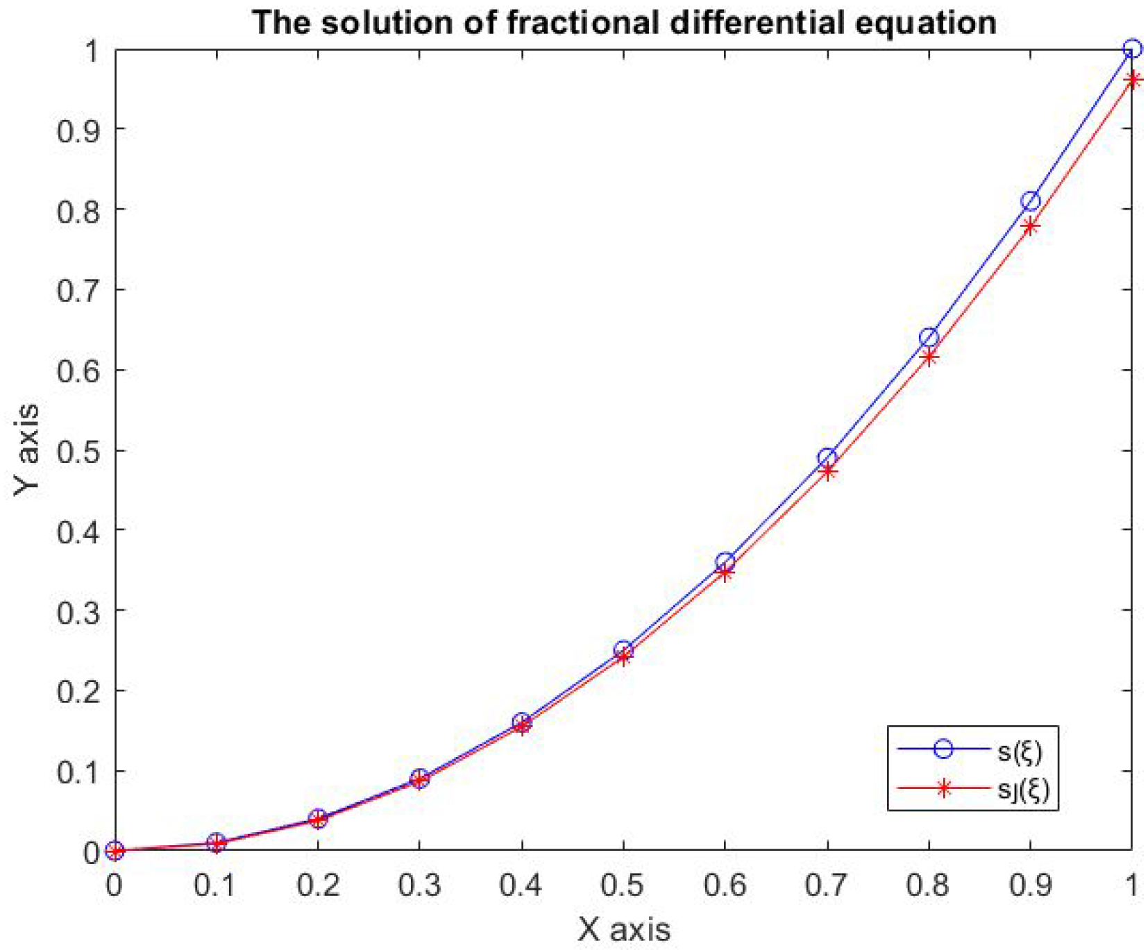
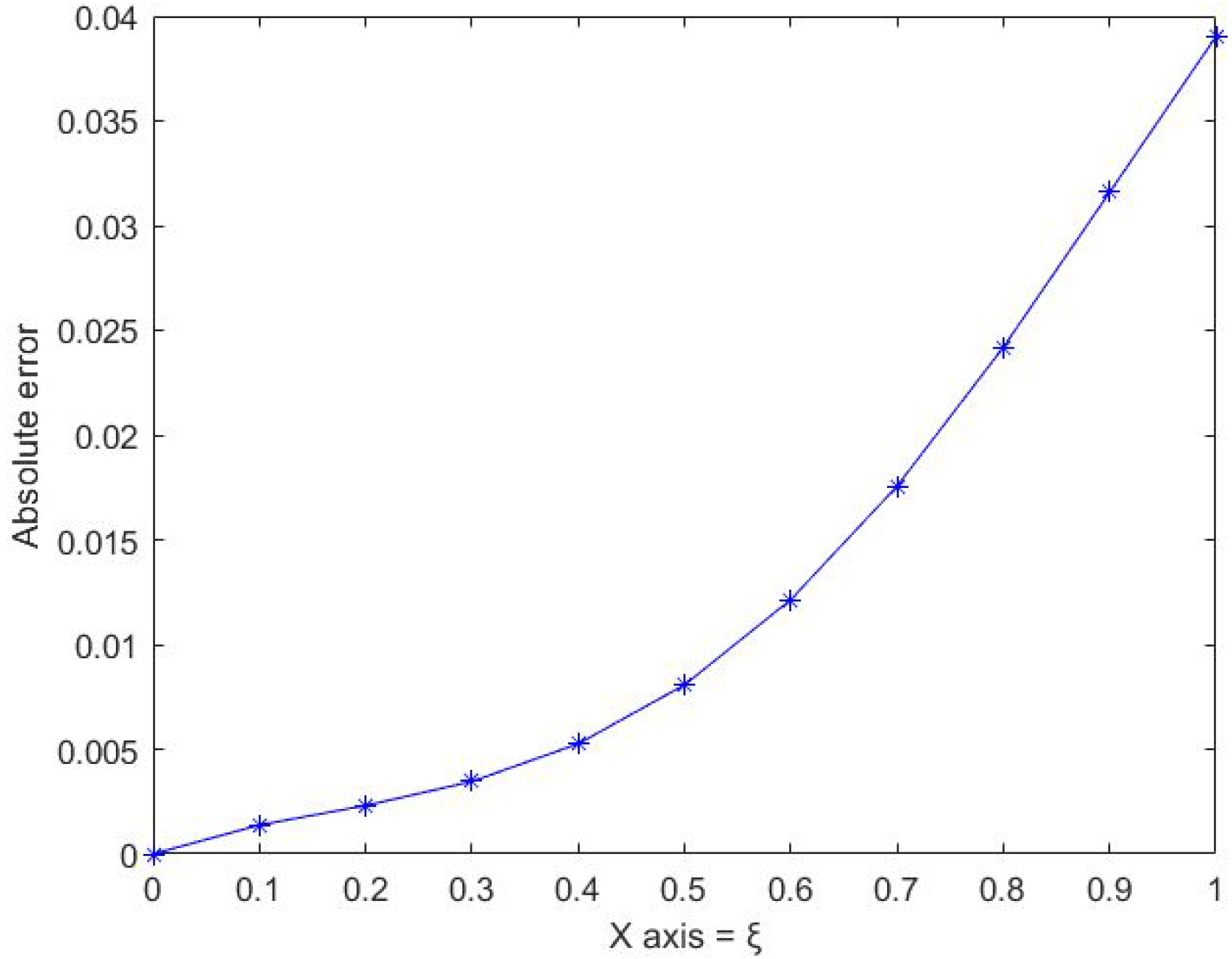
4.1. Fractional Differential Equations

For a function $\mathfrak{s}\in \mathcal{C}[0,1]$, the Riemann–Liouville fractional derivative of order $\delta >0,𝚥-1\le \delta \le 𝚥\in \mathbb{N}$ is given by

$$\begin{array}{c}\hfill \frac{1}{\mathsf{\Gamma }(𝚥-\delta )}\frac{d^{𝚥}}{d{\xi }^{𝚥}}{\int }_0^{\xi }\frac{\mathfrak{s}\left(\pi \right)d\pi }{{(\xi -\pi )}^{\delta -𝚥+1}}={\mathcal{D}}^{\delta }\mathfrak{s}\left(\xi \right),\end{array}$$

$\mathsf{\Gamma }$ is the Euler gamma function, given that the right-hand side is defined point-wise on [0, 1], where $\left[\delta \right]$ is the integer component of $\delta ,\mathsf{\Gamma }$. Consider the fractional differential equation as follows:

$$\begin{array}{cc}\hfill & {}^{\pi }{\mathcal{D}}^{\sigma }\mathfrak{s}\left(\xi \right)+\mathcal{X}(\xi ,\mathfrak{s}\left(\xi \right))=0,0\le \xi \le 1,0\le \sigma \le 1;\hfill \\ \hfill & \mathfrak{s}\left(0\right)=\mathfrak{s}\left(1\right)=0,\hfill \end{array}$$

(20)

where $\mathcal{X}:[0,1]\times \mathbb{R}\to \mathbb{R}$ is a continuous function and ${}^{\pi }{\mathcal{D}}^{\sigma }$ represents the Caputo fractional derivative of order $\sigma$ and is defined by

$$\begin{array}{c}\hfill {}^{\pi }{\mathcal{D}}^{\sigma }=\frac{1}{\mathsf{\Gamma }(𝚥-\sigma )}{\int }_0^{\zeta }\frac{{\mathfrak{s}}^{𝚥}\left(\pi \right)d\pi }{{(\xi -\pi )}^{\sigma -𝚥+1}},\end{array}$$

where $𝚥-1\le \sigma \le 𝚥\in \mathbb{N},\sigma \in \mathbb{R}$. Let $\mathcal{P},\mathcal{S}=\left(\mathcal{C}\right[0,1],[0,\infty \left)\right)$ be the set of all the continuous functions defined on $[0,1]$ with $[0,\infty )$. Consider $\phi :\mathcal{P}\times \mathcal{S}\to {\mathbb{R}}^{+}$ to be defined by

$$\begin{array}{c}\hfill \phi (\mathfrak{s},{\mathfrak{s}}^{\prime })=\underset{\xi \in [0,1]}{sup}{|\mathfrak{s}\left(\xi \right)-{\mathfrak{s}}^{\prime }\left(\xi \right)|}^2\end{array}$$

and $\mathsf{\Omega }(\mathfrak{s},{\mathfrak{s}}^{\prime })=3$ for all $(\mathfrak{s},{\mathfrak{s}}^{\prime })\in \mathcal{P}\times \mathcal{S}$. Then, $(\mathcal{P},\mathcal{S},\phi )$ is a complete bipolar controlled metric space.

Theorem 3.

Assume the nonlinear fractional differential equation (20). Suppose that the following conditions are satisfied:

1.

$\exists \xi \in [0,1]$,$\chi \in (0,1)$ and $(\mathfrak{s},{\mathfrak{s}}^{\prime })\in \mathcal{P}\times \mathcal{S}$ s.t

$$\begin{array}{c}\hfill |\mathcal{X}(\xi ,\mathfrak{s})-\mathcal{X}(\xi ,{\mathfrak{s}}^{\prime })|\le \sqrt{\chi }|\mathfrak{s}\left(\xi \right)-{\mathfrak{s}}^{\prime }\left(\xi \right)|;\end{array}$$

2.

$$\begin{array}{c}\hfill \underset{\xi \in [0,1]}{sup}{\int }_0^1{\left|\mathcal{G}(\xi ,\pi )\right|}^{2}d\pi \le 1.\end{array}$$

Then, the Equation (20) has a unique solution in $\mathcal{P}\cup \mathcal{S}$.

Proof. 

The given fractional differential equation (20) is equivalent to the succeeding integral equation with the orthogonal set $(\mathcal{W},\perp )$,

$$\begin{array}{c}\hfill \mathfrak{s}\left(\xi \right)={\int }_0^1\mathcal{G}(\xi ,\pi )\mathcal{X}(\mathfrak{q},\mathfrak{s}\left(\pi \right))d\pi ,\forall \xi ,\pi \in \mathcal{W}.\end{array}$$

Take the orthogonal function $\mathcal{G}(\xi ,\pi )$ with $\xi \perp \pi$,

$$\begin{array}{c}\hfill \mathcal{G}(\xi ,\pi )=\left\{\begin{array}{cc}\frac{{\left[\xi (1-\pi )\right]}^{\sigma -1}-{(\xi -\pi )}^{\sigma -1}}{\mathsf{\Gamma }\left(\sigma \right)},\hfill & 0\le \pi \le \xi \le 1,\hfill \\ \frac{{\left[\xi (1-\pi )\right]}^{\sigma -1}}{\mathsf{\Gamma }\left(\sigma \right)},\hfill & 0\le \xi \le \pi \le 1.\hfill \end{array}\right.\end{array}$$

Define the covariant mapping $\mathcal{T}:\mathcal{P}\cup \mathcal{S}\to \mathcal{P}\cup \mathcal{S}$ and $\mathcal{T}$ is orthogonal preserving. For each $\xi ,\pi \in \mathcal{W}$ with $\xi \perp \pi$ as defined by

$$\begin{array}{c}\hfill \mathcal{T}\mathfrak{s}\left(\xi \right)={\int }_0^1\mathcal{G}(\xi ,\pi )\mathcal{X}(\mathfrak{q},\mathfrak{s}\left(\pi \right))d\pi .\end{array}$$

It is easy to note that if ${\mathfrak{s}}^{*}\in \mathcal{T}$ is a fixed point then ${\mathfrak{s}}^{*}$ is a solution of the problem (20).

Let $\mathfrak{s},\mathfrak{s}\prime \in \mathcal{P}\times \mathcal{S}$ with $\mathfrak{s}\perp {\mathfrak{s}}^{\prime }$. Now,

$$\begin{array}{cc}\hfill |\mathcal{T}\mathfrak{s}\left(\xi \right)-\mathcal{T}{\mathfrak{s}}^{\prime }{\left(\xi \right)|}^2& =|{\int }_0^1\mathcal{G}(\xi ,\pi )\mathcal{X}(\mathfrak{q},\mathfrak{s}\left(\pi \right))d\pi -{\int }_o^1\mathcal{G}(\xi ,\pi )\mathcal{X}(\mathfrak{q},{\mathfrak{s}}^{\prime }\left(\pi \right))d\pi {|}^2\hfill \\ \hfill & \le {\int }_0^1{\left|\mathcal{G}(\xi ,\pi )\right|}^{2}d\pi ·{\int }_0^1|\mathcal{X}(\mathfrak{q},\mathfrak{s}\left(\pi \right))-\mathcal{X}(\mathfrak{q},{\mathfrak{s}}^{\prime }\left(\pi \right)){|}^{2}d\pi \hfill \\ \hfill & \le \chi |\mathfrak{s}\left(\xi \right)-{\mathfrak{s}}^{\prime }\left(\xi \right){|}^2.\hfill \end{array}$$

Taking the supremum on both sides, we obtain

$$\begin{array}{c}\hfill \phi (\mathcal{T}\mathfrak{s},\mathcal{T}{\mathfrak{s}}^{\prime })\le \chi \phi (\mathfrak{s},{\mathfrak{s}}^{\prime }).\end{array}$$

Hence, all the hypotheses of Theorem 1 are verified, and consequently, the fractional differential Equation (20) has a unique solution. □

Example 3.

The linear fractional differential equation is as follows:

$$\begin{array}{c}\hfill {}^{\pi }{\mathcal{D}}^{\sigma }\mathfrak{s}\left(\xi \right)+\mathfrak{s}\left(\xi \right)={\displaystyle \frac{2}{\mathsf{\Gamma }(3-\sigma )}}{\xi }^{2-\sigma }+{\xi }^3,\end{array}$$

(21)

where ${}^{\pi }{\mathcal{D}}^{\sigma }$ represents the Caputo fractional derivative of order σ with the initial condition: $\mathfrak{s}\left(0\right)=0,{\mathfrak{s}}^{\prime }\left(\mathfrak{0}\right)=0$.

The exact solution of Equation (21) with $\sigma =1.9$:

$$\begin{array}{c}\hfill \mathfrak{s}\left(\xi \right)={\xi }^2.\end{array}$$

Clearly, $\mathfrak{s}\left(\xi \right)$ is an orthogonal continuous function on [0, 1]. In virtue of Equation (20), we can write Equation (21) in the homotopy form;

$$\begin{array}{c}\hfill {\mathcal{D}}^{\sigma }\mathfrak{s}\left(\xi \right)+\mathfrak{p}\mathfrak{s}\left(\xi \right)-{\displaystyle \frac{2}{\mathsf{\Gamma }(3-\sigma )}}{\xi }^{2-\sigma }-{\xi }^3=0,\end{array}$$

(22)

the solution of Equation (21) is:

$$\begin{array}{c}\hfill \mathfrak{s}\left(\xi \right)={\mathfrak{s}}_0\left(\xi \right)+\mathfrak{p}{\mathfrak{s}}_1\left(\xi \right)+{\mathfrak{p}}^2{\mathfrak{s}}_2\left(\xi \right)+\cdots .\end{array}$$

(23)

Substituting Equation (23) into (22) and collecting terms with the power of $\mathfrak{p}$, we obtain

$$\left\{\begin{array}{cc}{\mathfrak{p}}^0:\hfill & {\mathcal{D}}^{\sigma }{\mathfrak{s}}_0\left(\xi \right)=0\hfill \\ {\mathfrak{p}}^1:\hfill & {\mathcal{D}}^{\sigma }{\mathfrak{s}}_1\left(\xi \right)=-{\mathfrak{s}}_0\left(\xi \right)+\mathfrak{X}\left(\xi \right)\hfill \\ {\mathfrak{p}}^2:\hfill & {\mathcal{D}}^{\sigma }{\mathfrak{s}}_2\left(\xi \right)=-{\mathfrak{s}}_1\left(\xi \right)\hfill \\ {\mathfrak{p}}^3:\hfill & {\mathcal{D}}^{\sigma }{\mathfrak{s}}_3\left(\xi \right)=-{\mathfrak{s}}_2\left(\xi \right)\hfill \\ & ⋮\hspace{1em}\hspace{1em}\hspace{1em}\hspace{1em}\hspace{1em}\hspace{1em}\hspace{1em}.\hfill \end{array}\right.$$

(24)

Applying ${\mathsf{\Omega }}^{\sigma }$ and the inverse operation of ${\mathcal{D}}^{\sigma }$, on both sides of Equation (24) and fractional integral operation $\left({\mathsf{\Omega }}^{\sigma }\right)$ of order $\sigma >0$, we have

$$\begin{array}{cc}\hfill {\mathfrak{s}}_0\left(\xi \right)& =\sum _{\mathfrak{i}=0}^1{\mathfrak{s}}^{\mathfrak{i}}\left(0\right){\displaystyle \frac{{\xi }^{\mathfrak{i}}}{\mathfrak{i}!}}\hfill \\ & =\mathfrak{s}\left(0\right){\displaystyle \frac{{\xi }^0}{0!}}+{\mathfrak{s}}^{\prime }\left(0\right){\displaystyle \frac{{\xi }^1}{1!}}\hfill \\ \hfill {\mathfrak{s}}_1\left(\xi \right)& =-{\mathsf{\Omega }}^{\sigma }\left[{\mathfrak{s}}_0\left(\xi \right)+{\mathsf{\Omega }}^{\sigma }\left[\mathfrak{X}\left(\xi \right)\right]\right]\hfill \\ & ={\xi }^2+{\displaystyle \frac{\mathsf{\Gamma }\left(4\right)}{\mathsf{\Gamma }(4+\sigma )}}{\xi }^{3+\sigma },\hfill \\ \hfill {\mathfrak{s}}_2\left(\xi \right)& =-{\mathsf{\Omega }}^{\sigma }\left[{\mathfrak{s}}_1\left(\xi \right)\right]\hfill \\ & ={\displaystyle \frac{2}{\mathsf{\Gamma }(3+\sigma )}}{\xi }^{2+\sigma }-{\displaystyle \frac{6}{\mathsf{\Gamma }(3+2\sigma )}}{\xi }^{3+2\sigma },\hfill \\ \hfill {\mathfrak{s}}_3\left(\xi \right)& =-{\mathsf{\Omega }}^{\sigma }\left[{\mathfrak{s}}_2\left(\xi \right)\right]\hfill \\ & ={\displaystyle \frac{2}{\mathsf{\Gamma }(3+2\sigma )}}{\xi }^{2+2\sigma }-{\displaystyle \frac{6}{\mathsf{\Gamma }(3+3\sigma )}}{\xi }^{3+3\sigma }.\hfill \end{array}$$

Hence, the solution of Equation (21) is

$$\begin{array}{cc}\mathfrak{s}\left(\xi \right)\hfill & ={\mathfrak{s}}_0\left(\xi \right)+{\mathfrak{s}}_1\left(\xi \right)+{\mathfrak{s}}_2\left(\xi \right)+\cdots \hfill \end{array}$$

(25)

$$\begin{array}{cc}\hfill \mathfrak{s}\left(\xi \right)& ={\xi }^2+{\displaystyle \frac{\mathsf{\Gamma }\left(4\right)}{\mathsf{\Gamma }(4+\sigma )}}{\xi }^{(3+\sigma )}-{\displaystyle \frac{2}{\mathsf{\Gamma }(3+\sigma )}}{\xi }^{(2+\sigma )}-{\displaystyle \frac{6}{\mathsf{\Gamma }(4+2\sigma )}}{\xi }^{(3+2\sigma )}+\cdots ,\hfill \end{array}$$

(26)

when $\sigma =1.9$

$$\begin{array}{cc}\hfill \mathfrak{s}\left(\xi \right)& ={\xi }^2+{\displaystyle \frac{6}{\mathsf{\Gamma }\left(5.9\right)}}{\xi }^{\left(4.9\right)}-{\displaystyle \frac{2}{\mathsf{\Gamma }\left(4.9\right)}}{\xi }^{\left(3.9\right)}-{\displaystyle \frac{6}{\mathsf{\Gamma }\left(7.8\right)}}{\xi }^{\left(6.8\right)}+\cdots \hfill \\ & ={\xi }^2-\mathit{small}\mathit{terms}\hfill \\ & \approx {\xi }^2.\hfill \end{array}$$

Table 1. The numerical and exact solution using the matrix approach method.

$\mathit{\xi }$	$\mathfrak{s}\left(\mathit{\xi }\right)$	${\mathfrak{s}}_{𝚥}\left(\mathit{\xi }\right)$	$|\mathfrak{s}\left(\mathit{\xi }\right)-{\mathfrak{s}}_{𝚥}\left(\mathit{\xi }\right)|$
0.00000	0.00000	0.00000	0.00000
0.10000	0.01000	0.00862	0.00138
0.20000	0.04000	0.03769	0.00231
0.30000	0.09000	0.08654	0.00346
0.40000	0.16000	0.15474	0.00526
0.50000	0.25000	0.24193	0.00807
0.60000	0.36000	0.34786	0.01214
0.70000	0.49000	0.47244	0.01756
0.80000	0.64000	0.61581	0.02419
0.90000	0.81000	0.77841	0.03159
1.00000	1.00000	0.96098	0.03902

displays the numerical and exact results using the matrix approach method with $\sigma =1.9$ and $\mathcal{N}=51$.

Figure 1 compares both the numerical and exact solutions for the fractional differential Equation (21). Moreover, Figure 2 shows the absolute error between the numerical and exact solutions.

The exact and absolute solution is an equal value of 0 in this case. Therefore, the unique solution to this problem is 0. Hence the unique fixed point at 0.

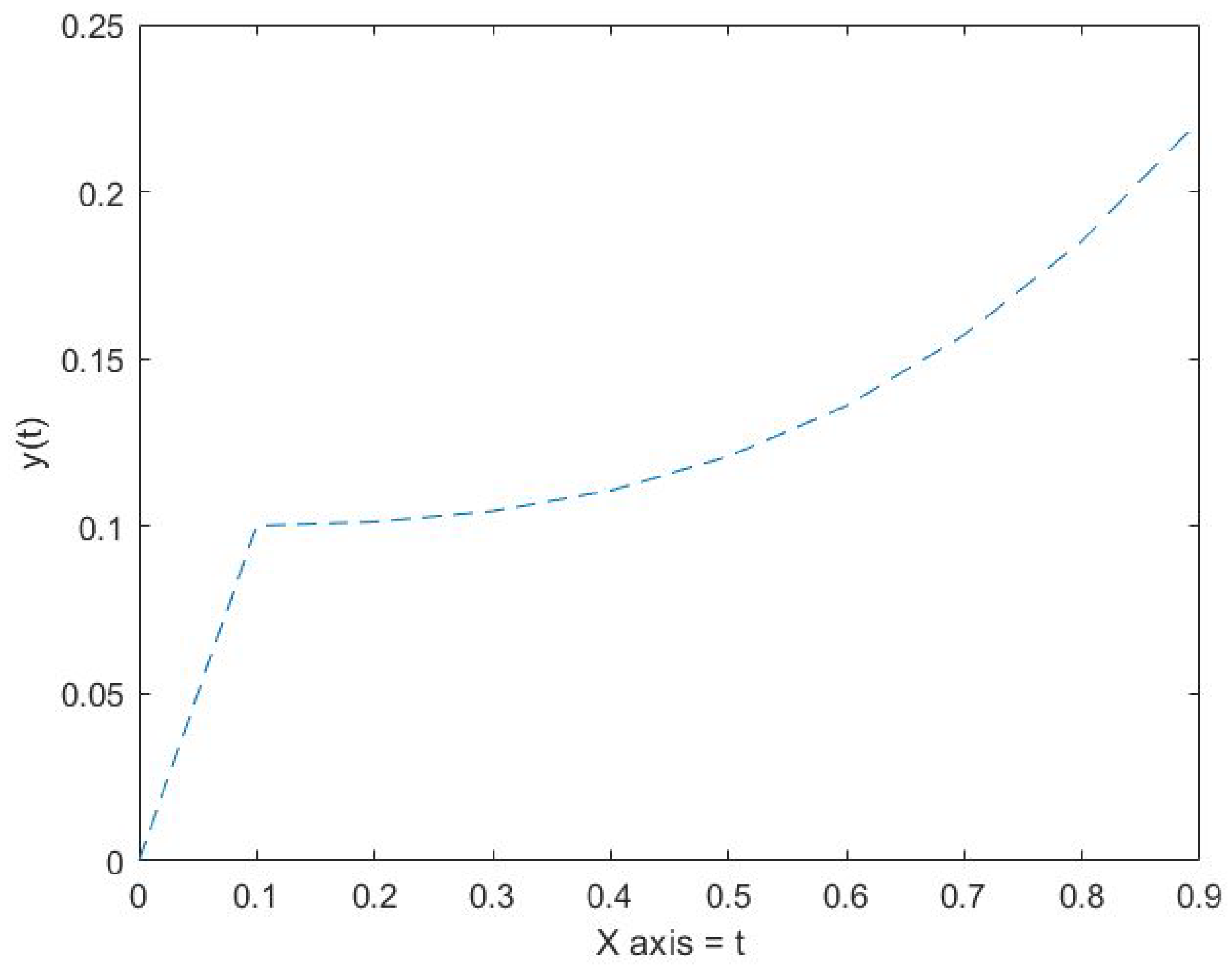
4.2. Application of Elzaki Transformation

We prove the convolution of the Elzaki transform by a different method with Elzaki.

$$\begin{array}{c}\hfill E(\mathfrak{X}★\mathfrak{g})={\displaystyle \frac{1}{\mathfrak{a}}}E\left(\mathfrak{X}\right)E\left(\mathfrak{g}\right)\end{array}$$

for $E\left(\mathfrak{X}\right)$ is the Elzaki transform of $\mathfrak{X}$. In general, we can find the solution by using the Elzaki transform as follows:

Theorem 4.

Let us consider the Volterra integral equation of the second kind as follows:

$$\begin{array}{c}\hfill \iota (\ell )=\varrho (\ell )+{\int }_a^{\ell }\mathit{K}(\ell -t)\iota \left(t\right)dt.\end{array}$$

(27)

It can be expressed as

$$\begin{array}{c}\hfill \iota (\ell )=E^{-1}\left(\mathcal{T}\left(\mathfrak{a}\right)\right)=E^{-1}\left({\displaystyle \frac{\mathfrak{a}\mathcal{X}}{\mathfrak{a}-\mathit{K}}}\right),\end{array}$$

where $\mathit{K}$ is the kernel and $E\left[\iota \right(\ell \left)\right]=\mathcal{T}\left(\mathfrak{a}\right)$.

Proof. 

Let $E\left[\iota \right(\ell \left)\right]=\mathcal{T}\left(\mathfrak{a}\right),E\left(\mathfrak{r}\right)=\mathcal{L}$ and $E\left(\mathfrak{q}\right)=\mathcal{T}$. If $\mathfrak{X}\left(\iota \right(\ell \left)\right)=\mathfrak{r}(\ell )$ is given, define the orthogonal relation ⊥ on $\mathcal{W}$ by

$$\begin{array}{c}\hfill \mathfrak{r}\perp \mathfrak{q}\mathrm{or}\mathfrak{q}\perp \mathfrak{r}.\end{array}$$

let us take both sides on the Elzaki transform; we have

$$\begin{array}{c}\hfill \mathcal{T}\left(\mathfrak{a}\right)={\displaystyle \frac{1}{\mathfrak{a}}}E\left(\mathfrak{r}\right)E\left(\mathfrak{q}\right)={\displaystyle \frac{1}{\mathfrak{a}}}\mathcal{L}\mathcal{T},\end{array}$$

for $\mathcal{T}$ is the transfer function. If we take the inverse Elzaki transform, we obtain

$$\begin{array}{c}\hfill \iota ={\mathcal{T}}^{-1}\left(\mathfrak{a}\right)=\mathfrak{r}★\mathfrak{q}={\mathcal{T}}^{-1}\left({\displaystyle \frac{1}{\mathfrak{a}}}\mathcal{L}\mathcal{T}\right),\forall \mathfrak{r}\perp \mathfrak{q},\end{array}$$

for ★ is the standard notation of convolution.

Let us take the Elzaki transform on Equation (27). Then we obtain

$$\begin{array}{c}\hfill \mathcal{T}\left(\mathfrak{a}\right)=\mathcal{X}=E(\iota ★\mathfrak{r})=\mathcal{X}+{\displaystyle \frac{1}{\mathfrak{a}}}\mathcal{T}\left(\mathfrak{a}\right)\mathit{K},\forall \iota \perp \mathfrak{r},\end{array}$$

for $\mathcal{X}=E\left(\varrho \right)$ and for $\mathit{K}=E\left(\mathfrak{r}\right)$ is orthogonal continuous. Organizing the equality, we obtain

$$\begin{array}{c}\hfill \mathcal{T}\left(\mathfrak{a}\right)={\displaystyle \frac{\mathfrak{a}\mathcal{X}}{\mathfrak{a}-\mathit{K}}},\end{array}$$

for the kernel. Therefore, we obtain

$$\begin{array}{c}\hfill \iota (\ell )=E^{-1}\left(\mathcal{T}\left(\mathfrak{a}\right)\right)=E^{-1}\left({\displaystyle \frac{\mathfrak{a}\mathcal{X}}{\mathfrak{a}-\mathit{K}}}\right).\end{array}$$

□

Example 4.

Let us consider the Volterra integral equation

$$\begin{array}{c}\hfill \iota (\ell )-{\int }_0^{\ell }t\iota (\ell -t)dt=1.\end{array}$$

(28)

Solution.Writing

$$\begin{array}{c}\hfill \iota -\ell ★\iota =1,\end{array}$$

for $\iota \perp \ell$, we obtain

$$\begin{array}{c}\hfill \mathcal{T}\left(\mathfrak{a}\right)-{\displaystyle \frac{1}{\mathfrak{a}}}E(\ell )\mathcal{T}\left(\mathfrak{a}\right)=E\left(1\right),\end{array}$$

for $E\left[\iota \right(\ell \left)\right]=\mathcal{T}\left(\mathfrak{a}\right)$. From the table of the Elzaki transform

Table A1. Elzaki transform of some functions.

t	$\mathit{\chi }\left(\mathfrak{a}\right)$
1	${\mathfrak{a}}^2$
t	${\mathfrak{a}}^3$
${\displaystyle \frac{t^3}{6}}$	${\mathfrak{a}}^5$
$t^{𝚥}$	$𝚥!{\mathfrak{a}}^{𝚥+2}$
$e^{bt}$	${\displaystyle \frac{{\mathfrak{a}}^2}{1-b\mathfrak{a}}}$
$sin\left(bt\right)$	${\displaystyle \frac{b{\mathfrak{a}}^3}{1+b^2{\mathfrak{a}}^2}}$

in Appendix A, we obtain

$$\begin{array}{c}\hfill \mathcal{T}\left(\mathfrak{a}\right)-{\displaystyle \frac{1}{\mathfrak{a}}}{\mathfrak{a}}^3\mathcal{T}\left(\mathfrak{a}\right)={\mathfrak{a}}^2.\end{array}$$

Arranging the inequality, we obtain

$$\begin{array}{c}\hfill \mathcal{T}\left(\mathfrak{a}\right)={\displaystyle \frac{{\mathfrak{a}}^2}{1-{\mathfrak{a}}^2}}.\end{array}$$

Taking the inverse Elzaki transform, we obtain

$$\begin{array}{c}\hfill \iota (\ell )=cos(h\ell ),\end{array}$$

for h is a hyperbolic function.

It is a well-known fact that the first order ODE

$$\begin{array}{c}\hfill {\displaystyle \frac{d\iota }{d\varrho }}=\mathfrak{X}(\varrho ,\iota ),\forall \varrho \perp \iota ,\end{array}$$

with the condition $\iota \left(a\right)={\iota }_0$ is rewritten to

$$\begin{array}{c}\hfill \varphi \left(\varrho \right)={\iota }_0+{\int }_a^{\varrho }\mathfrak{X}(\ell ,\varphi (\ell ))d\ell ,\end{array}$$

where $\mathfrak{X}$ is orthogonal continuous and contains the point $(a,{\iota }_0)$. Similarly, an initial value problem

$$\begin{array}{c}\hfill {\iota }^{″}+A(\ell ){\iota }^{\prime }+B(\ell )\iota =0\end{array}$$

with the condition $\iota \left(a\right)={\iota }_0,{\iota }^{\prime }\left(a\right)={\iota }_1$ is rewritten to the Volterra integral equation of the second kind

$$\begin{array}{c}\hfill \iota (\ell )=\mathfrak{X}(\ell )+{\int }_a^{\ell }K(\ell ,t)\iota \left(t\right)dt,\end{array}$$

(29)

where $K(\ell ,t)=-A\left(t\right)+(t-\ell )(B\left(t\right)-A^{\prime }\left(t\right)).$ Additionally, the above $\mathfrak{X}(\ell )$ is orthogonal continuous on $[a,b]$ and the kernel K is orthogonal continuous on the triangular region R in the $\ell t$-plane given by $a\le t\le \ell ,a\le \ell \le b$. Then we know that (29) has a unique solution ι on $[a,b]$.

Example 5.

Solve the Volterra integral equation

$$\begin{array}{c}\hfill \iota (\ell )={\int }_0^{\ell }\iota \left(t\right)sin(\ell -t)dt=\ell .\end{array}$$

Solution.The given equation can be written by

$$\begin{array}{c}\hfill \iota -\iota ★sin\ell =\ell ,\end{array}$$

for $\ell \perp t,\ell \in [0,1]$. Let us write $E\left[\iota \right(\ell \left)\right]=\mathcal{T}\left(\mathfrak{a}\right)$ and apply the convolution theorem. Then, we obtain

$$\begin{array}{c}\hfill \mathcal{T}\left(\mathfrak{a}\right)-{\displaystyle \frac{1}{\mathfrak{a}}}\mathcal{T}\left(\mathfrak{a}\right){\displaystyle \frac{{\mathfrak{a}}^3}{1+{\mathfrak{a}}^2}}={\mathfrak{a}}^3.\end{array}$$

We obtain

$$\begin{array}{cc}\hfill \mathcal{T}\left(\mathfrak{a}\right)& ={\mathfrak{a}}^3(1+{\mathfrak{a}}^2)\hfill \\ & ={\mathfrak{a}}^3+{\mathfrak{a}}^5\hfill \end{array}$$

As we scan a table of Elzaki transformations Table A1, we obtain

$$\begin{array}{c}\hfill \iota (\ell )=\ell +{\displaystyle \frac{{\ell }^3}{6}}.\end{array}$$

It is clear that $\iota (\ell )$ is orthogonal continuous on $[0,1]$. Its shown in Figure 3 as follow:

5. Conclusions

In this paper, we proved some fixed point theorems for an orthogonal Istr$\breve{a}$tescu type contraction of maps in an orthogonal CbMS. Furthermore, we presented examples that elaborated on the usability of our results. Meanwhile, we provided applications to the existence of a solution for a fractional differential equation and second kind Volterra integral equation through an Elzaki transform by using our main results.

References

1. Banach, S. Sur les operations dans les ensembles abstraits et leurs applications aux equations integrales. Fundam. Math. 1992, 3, 133–181. [Google Scholar] [CrossRef]
2. Shatanawi, W. On w-compatible mappings and common coupled coincidence point in cone metric spaces. Appl. Math. Lett. 2012, 25, 925–931. [Google Scholar] [CrossRef] [Green Version]
3. Shatanawi, W.; Rajic, R.V.; Radenovic, S.; Al-Rawashhdeh, A. Mizoguchi-Takahashi-type theorems in tvs-cone metric spaces. Fixed Point Theory Appl. 2012, 11, 106. [Google Scholar] [CrossRef] [Green Version]
4. Al-Rawashdeh, A.; Hassen, A.; Abdelbasset, F.; Sehmim, S.; Shatanawi, W. On common fixed points for α-F-contractions and applications. J. Nonlinear Sci. Appl. 2016, 9, 3445–3458. [Google Scholar] [CrossRef] [Green Version]
5. Shatanawi, W.; Mustafa, Z.; Tahat, N. Some coincidence point theorems for nonlinear contraction in ordered metric spaces. Fixed Point Theory Appl. 2011, 2011, 68. [Google Scholar] [CrossRef] [Green Version]
6. Shatanawi, W. Some fixed point results for a generalized Ψ-weak contraction mappings in orbitally metric spaces. Chaos Solitons Fractals 2012, 45, 520–526. [Google Scholar] [CrossRef]
7. Istrătescu, V. Some fixed point theorems for convex contraction mappings and mappings with convex diminishing diameters (I). Ann. Mat. Pura Appl. 1982, 130, 89–104. [Google Scholar]
8. Istrătescu, V. Some fixed point theorems for convex contraction mappings and mappings with convex diminishing diameters (II). Ann. Mat. Pura Appl. 1983, 134, 327–362. [Google Scholar]
9. Berinde, V. Approximating fixed points of weak contractions using the Picard iteration. Nonlinear Anal. Forum 2004, 9, 43–53. [Google Scholar]
10. Bakhtin, I.A. The contraction mapping principle in quasimetric spaces. J. Funct. Anal. 1989, 30, 26–37. [Google Scholar]
11. Czerwik, S. Nonlinear set-valued contraction mappings in b-metric spaces. Atti Del Semin. Mat. Fis. Dell’Universita Modena 1998, 46, 263–276. [Google Scholar]
12. Hussain, N.; Doric, D.; Kadelburg, Z.; Radenovi´c, S. Suzuki-type fixed point results in metric type spaces. J. Inequalities Appl. 2014, 2014, 229. [Google Scholar] [CrossRef] [Green Version]
13. Latif, A.; Al Subaie, R.F.; Alansari, M.O. Fixed points of generalized multi-valued contractive mappings in metric type spaces. J. Nonlinear Var. Anal. 2022, 6, 123–138. [Google Scholar]
14. Haghi, R.H.; Bakhshi, N. Some coupled fixed point results without mixed monotone property. J. Adv. Math. Stud. 2022, 15, 456–463. [Google Scholar]
15. Yao, Y.; Shahzad, N.; Yao, J.C. Convergence of Tseng-type self-adaptive al-gorithms for variational inequalities and fixed point problems. Carpathian J. Math. 2021, 37, 541–550. [Google Scholar] [CrossRef]
16. Gordji, M.E.; Habibi, H. Fixed point theory in generalized orthogonal metric space. J. Linear Topol. Algebra 2017, 6, 251–260. [Google Scholar]
17. Aiman, M.; Arul Joseph, G.; Absar, U.H.; Senthil Kumar, P.; Gunaseelan, M.; Imran, A.B. Solving an Integral Equation via Orthogonal Brianciari Metric Spaces. J. Funct. Spaces 2022, 2022, 7251823. [Google Scholar]
18. Gnanaprakasam, A.J.; Mani, G.; Lee, J.R.; Park, C. Solving a nonlinear integral equation via orthogonal metric space. AIMS Math. 2022, 7, 1198–1210. [Google Scholar] [CrossRef]
19. Mani, G.; Gnanaprakasam, A.J.; Kausar, N.; Munir, M. Orthogonal F-Contraction mapping on O-Complete Metric Space with Applications. Int. J. Fuzzy Log. Intell. Syst. 2021, 21, 243–250. [Google Scholar] [CrossRef]
20. Arul Joseph, G.; Gunaseelan, M.; Vahid, P.; Hassen, A. Solving a Nonlinear Fredholm Integral Equation via an Orthogonal Metric. Adv. Math. Phys. 2021, 2021, 8. [Google Scholar]
21. Prakasam, S.K.; Gnanaprakasam, A.J.; Kausar, N.; Mani, G.; Munir, M. Solution of Integral Equation via Orthogonally Modified F-Contraction Mappings on O-Complete Metric-Like Space. Int. J. Fuzzy Log. Intell. Syst. 2022, 22, 287–295. [Google Scholar] [CrossRef]
22. Senthil Kumar, P.; Arul Joseph, G.; Ege, O.; Gunaseelan, M.; Haque, S.; Mlaiki, N. Fixed point for an 𝕆g𝔗-c in 𝕆-complete b-metric-like spaces. AIMS Math. 2022, 8, 1022–1039. [Google Scholar]
23. Gnanaprakasam, A.J.; Nallaselli, G.; Haq, A.U.; Mani, G.; Baloch, I.A.; Nonlaopon, K. Common Fixed-Points Technique for the Existence of a Solution to Fractional Integro-Differential Equations via Orthogonal Branciari Metric Spaces. Symmetry 2022, 14, 1859. [Google Scholar] [CrossRef]
24. Mani, G.; Prakasam, S.K.; Gnanaprakasam, A.J.; Ramaswamy, R.; Abdelnaby, O.A.A.; Khan, K.H.; Radenović, S. Common Fixed Point Theorems on Orthogonal Branciari Metric Spaces with an Application. Symmetry 2022, 14, 2420. [Google Scholar] [CrossRef]
25. Miculescu, R.; Mihail, A. New fixed point theorems for set-valued contractions in b-metric spaces. J. Fixed Point Theory Appl. 2017, 19, 2153–2163. [Google Scholar] [CrossRef]
26. Popescu, O. Some new fixed point theorems for a α Geraghty-contraction type maps in metric spaces. Fixed Point Theory Appl. 2014, 2014, 190. [Google Scholar] [CrossRef]
27. Gordji, M.E.; Ramezani, M.; De La Sen, M.; Cho, Y.J. On orthogonal sets and Banach fixed point theorem. Fixed Point Theory 2017, 18, 569–578. [Google Scholar] [CrossRef]
28. Ramezani, M. Orthogonal metric space and convex contractions. Int. J. Nonlinear Anal. Appl. 2015, 6, 127–132. [Google Scholar]
29. Karapinar, E.; Fulga, A.; Petrusel, A. On Istr a ˘ tescu Type contraction in b-Metric Space. Mathematics 2020, 8, 388. [Google Scholar] [CrossRef] [Green Version]
Figure 1. The convergence between an approximate and exact solution with an interval difference of 0.1 for Example 3.
Mathematics 11 00677 g001
Figure 2. The absolute error with an interval difference of 0.1 for Example 3.
Mathematics 11 00677 g002
Figure 3. Graph of ι ( ) with an interval difference of 0.1 for Example 5.
Mathematics 11 00677 g003