Exploring the Contagion Effect from Developed to Emerging CEE Financial Markets

Abstract

The paper aims to analyze the contagion effect coming from the developed stock markets of the US and Germany to the emerging CEE stock markets of Romania, Czech Republic, Hungary, and Poland using daily data for the period April 2005–April 2021. The paper also captures the level of integration of these emerging stock markets by analyzing the volatility spillover phenomenon. The quantification of the contagion effect coming from the developed to the emerging stock markets consisted of an empirical analysis based on the DCC-GARCH (Dynamic Conditional Correlation) model. Through this multivariate model, the time-varying conditional correlations were analyzed, both in periods of normal economic development and in times of economic instability, when there was a significant increase in the correlation coefficients between developed and emerging stock market indices. Furthermore, the level of connectedness between these markets has been analyzed using the volatility spillover index developed by Diebold and Yilmaz. The empirical results surprised the high level of integration of the analyzed stock markets in Central and Eastern Europe, with the intensity of volatility transmission between these markets increasing significantly during times of crisis. All stock market indices analyzed show periods during which they transmit net volatility and periods during which they receive net volatility, indicating a bidirectional volatility spillover phenomenon. Mostly, the BET, PX, and WIG indices are net transmitters of volatilities, whereas the BUX index is net recipient, except during the COVID-19 crisis, when it transmitted net volatility to the other three indices. Finally, using a Markov switching-regime VAR approach with two regimes, we explored the contagion effect between emerging CEE and developed stock markets during the COVID-19 pandemic. The empirical results proved a shift around the outbreak of the health crisis, after which the high volatility regime dominates the CEE markets. The contagion effects from developed stock markets to emerging CEE markets significantly increased during the first stage of the health crisis.

1. Introduction

In recent decades, interconnections between countries have increased substantially worldwide due to intensifying integration and globalisation. On the one hand, this has had a positive impact on economic development, but on the other hand, the strengthening of these links has made integrated countries more prone to external shocks, thus observing the phenomenon of financial contagion.

Decision-makers would be better equipped to respond quickly to financial shocks through appropriate policies if they were aware of the time-varying nature of stock market correlations, particularly during tumultuous times when financial markets are under pressure. Co-movements between asset returns that are more pronounced might reduce the benefit of globally diversified investment portfolios.

According to [1,2], the foundation of a global portfolio diversification approach is a low international correlation across markets. Losses in one stock are likely followed by losses in other stocks if there is a significant correlation between stock returns. Diversification benefits are larger when there is no connection between stock return trends. An increased correlation of stock market returns can be seen as the existence of the contagion effect.

The global scale of the stock market crash in October 1987, the Asian crisis in 1997, and the Russian default in 1998 have fueled a growing interest among researchers and policymakers in investigating the various aspects of international stock market relations, as the findings are essential both in the application of passive and active international in- vestment strategies and the identification of shock transmission channels.

As a result of the financial crisis of 2007–2009, the topic of stock market contagion has resurfaced. The events that began in the US subprime mortgage market and subsequently erupted into credit and the financial crisis have had a significant impact on the CEE nations. As a result of the financial crisis of 2007–2009, investors in over-leveraged speculative hedge funds and private equity, as well as other institutional investors, have pulled practically all their money out of developing countries, particularly the CEE stock markets. Faced with bankruptcy, these institutional investors sold most of their CEE and other emerging market equities, bonds, and currencies and replaced them with safer assets, such as US government bonds. According to the definition given by [3] Dornbusch, Park, and Claessens (2000), contagion refers to the spread of market disturbances—especially those with negative impact—from one country to another, a process observed through co-movements in exchange rates, stock, and bond prices and capital flows, while [4] Forbes and Rigobon (2002) defined it as an increase in the intensity of market connections after a shock.

Although there is comprehensive literature exploring the links among developed stock markets, there are a relatively limited number of studies in the literature analyzing the linkages between emerging and developed countries([5], Yang, 2005; [6], Chiang, Jeon, & Li, 2007; [7] Phylaktis & Ravazzolo, 2005; [8] Syllignakis & Kouretas, 2011; [9] Grabowski, 2011; or [10] Horvath et al., 2017), with differences and similarities in terms of the period span, the sample of countries, and the methods applied to capture the contagion effect, which are all intended to capture a multilateral image of the same phenomenon.

Syllignakis and Kouretas (2011) [8] provided evidence of contagion effects among the US, German, and Russian stock markets and the CEE stock markets, using a sample of 7 emerging countries from 1997–2009.

Grabowski (2019) [11] used the period May 2004–June 2019 to analyse co-movements between the stock markets of Poland, the Czech Republic, Hungary, and the three developed nations (the US, Germany, and Spain). The empirical findings demonstrated that the CEE nations had been receivers of volatility from Germany, the US, and Spain during the euro area sovereign debt crisis between 2004 and 2019. Volatility transmission to Poland, the Czech Republic, and Hungary drastically decreased after 2012.

Using the definition of [12] Bae, Karolyi, and Stulz (2003), [11] Horvath et al. (2017) examined the contagion from the US stock market to six CEE stock markets using a novel measure of contagion, proving the existence of financial contagion and revealing that unexpected adverse events in the US market are followed by higher co-exceedance between US and Central and Eastern European stock markets. Even though contagion is stronger during the financial crisis, it also occurs in quiet times.

Samarakoon (2011) [13] investigates the transmission of the financial crisis from the US stock market to 62 developing and frontier stock markets, including those of the CEE area, demonstrating the lack of contagion and rather high sensitivity of emerging markets to developments in the US market. In their 2015 study on time-varying dependency across multiple CEE markets (Hungary, the Czech Republic, Poland, and Romania), Reboredo, Tiwari, and Albulescu demonstrate that this dependence grew during the most recent financial crisis.

The relevance of stressing the existence of contagion effects increases if we recognize the importance of monitoring the stock markets’ performance related to the domestic stock market even more during the COVID-19 epidemic. The industrialized and developing world economies, notably the financial markets, have been altered by the COVID-19 pandemic ([14], Siddiqui et al., 2022). Pandemics affect financial systems through huge economic costs ([15], Goodell, 2020). However, research that examines the effects of pandemics on financial markets is rather limited. According to So et al. (2020) [16], the COVID-19 epidemic impacts the level of correlation in stock returns in the Hong Kong market.

In contrast to earlier financial crises, the COVID-19 epidemic has resulted in a significant increase in the network connectivity of financial networks. Albulescu (2021) [17] investigates how the public disclosure of new confirmed cases and the mortality rate affects the volatility of US stock markets. As a result of COVID-19, the S&P 500 stock volatility has increased, according to their findings.

Although the number of studies that treat the contagion effect in Eastern European countries or the effects of pandemics in relation to the CEE financial markets are increasing, the body of literature needs to be expanded overall. It is, therefore, worthwhile to analyze the contagion effect among CEE stock markets, including the major shock of the sanitary crisis.

The study aims to add to the body of knowledge on contagion by looking at shocks that occurred during the last decades (the financial crisis 2008–2009, the European sovereign debt crisis, the US–China trade war, and the health crisis caused by COVID-19) in developed markets and developing economies. Therefore, this paper aims to identify the impact of crisis periods on the evolution of correlation coefficients between the developed stock markets (such as Germany and the US) and the stock markets in Central and Eastern Europe (Romania, Czech Republic, Hungary, and Poland). Furthermore, the contagion between the stock indices of the CEEC countries is analyzed through the effect of volatility spillover, thereby demonstrating the interconnections between these markets. In order to achieve all these, the DCC-GARCH (Dynamic Conditional Correlation) model and Diebold–Yilmaz (2012) methodology are applied in combination with the Markov switching regime approach.

This paper makes several contributions to the relevant literature. Firstly, longer time series have been used in this empirical analysis, capturing the volatilities of the first year of pandemics. The period April 2004–April 2021 has been considered. Second, previous research studies have concentrated either on the impact of the EU accession, US subprime crisis, the financial crisis, or the euro area sovereign debt crisis on stock markets or either from the relatively few ones that target the COVID pandemic in emerging countries that are not part of the CEE ([14], Siddiqui et al., 2022; [18], Nguyen et al. 2022). Therefore, there is still a critical gap addressed in this paper, quantifying the contagion effect from developed stock markets to CEE countries, chronologically accounting for a succession of crises, including the specificities of the last major crisis: the health crisis. Third, we employed the Dynamic Conditional Correlation (DCC) multivariate GARCH models to investigate the short-run interdependencies pattern and examine potential channels of contagion effects between the CEE and the US and German stock markets. An advantage of the multivariate DCC–GARCH model is that we can obtain all possible pair-wise correlation coefficients for the index returns in the sample and study their behaviour during periods of particular interest, such as the sanitary crisis. In the estimation of multivariate models, we have incorporated the different time zones in which the European and the US stock markets are traded, considering that largely cross-correlations are registered when the European market returns are taken one calendar day delayed relative to the US market. Therefore, we have also estimated the German stock market models without delay and compared the results.

Fourth, an important contribution within the paper regards quantifying the contagion effect in times of crisis based on the dummy variable approach of [8] Syllignakis and Kouretas (2011); three crises are considered, with the health crisis being the one that has the greatest element of novelty. It is worth mentioning that the crisis periods have been determined based on economic events with a major impact on the stock market and by analyzing the VIX index and the Composite Indicator of Systemic Stress (CISS). Six, this paper utilizes the spillover index approach of [19] Diebold and Yilmaz (2012) to assess the magnitude and direction of connectedness between stock markets, taking into account the recent sanitary crisis. The main advantage of this technique is that it offers information on the direction and magnitude of risk spillover, helping investors to make appropriate investment decisions. The rolling sample approach also allows us to examine the risk spillovers over time without using a cutoff date to create subsamples.

Finally, using a Markov switching-regime VAR approach with two regimes, we explored the contagion effect between CEE stock markets and developed stock markets during the COVID-19 pandemic, assuming that the effects of shocks may occasionally lead to regime transitions. Based on the generalized impulse response functions and variance decomposition analysis, the effects of a shock from the developed stock markets to the CEE stock markets have been isolated.

This paper is structured as follows. The literature review section highlights the effect of financial contagion in literature, including the papers that capture this phenomenon in the stock markets of Central and Eastern Europe. Section 3 summarizes the main characteristics of the CEEC stock markets included in the analysis. The data section illustrates the main data used and the associated descriptive statistics. The next three sessions describe the DCC-GARCH methodology, the volatility spillover index implemented by Diebold-Yilmaz (2012), and the Markov switching regime approach together with the empirical results. Finally, the paper ends with major conclusions, implications for investors and policy makers, and future research directions.

2. Exploring the Financial Contagion Phenomenon within the Literature

The literature on the contagion between international stock markets is extensive. It is thoroughly documented that, over time, the correlation between stock indices has varied significantly, especially in times of crisis. The October 1987 stock market crash in the US, the 1997 Asian financial crisis, and the 1998 Russian financial crisis gave rise to numerous empirical analyses on how shocks are transmitted to global financial markets.

One of the first papers on contagion in the stock markets was written by [20] King and Wadhwani (1990). They analyzed stock indices (high-frequency data) in the United States, the United Kingdom, and Japan over eight months (July 1987–February 1988). As a result, the authors identified significant increases in correlation coefficients between these markets as early as October 1987, when the Dow Jones index recorded the highest decline (of 22.6%) (US stock market crash, 1987). Lee and Kim (1993) [21] extended this analysis to 12 stock market indices for the period 1985–1990 and found other evidence of contagion: the average weekly correlations between stock markets increased from 0.22 (before the collapse of the 1987 US stock market) to 0.38 after the crisis.

Numerous studies have looked at conditional correlations to study financial market contagion ([22], Akhtaruzzaman et al., 2021; [6], Chiang et al., 2007; [23], Dimitriou et al., 2013; [24], Hwang et al., 2013; [25] Min and Hwang, 2012; [26] Yousfi et al., 2021). However, it is not always easy to separate contagion from correlation dynamics. [4] Forbes and Rigobon (2002) analyzed the correlations between stock markets in different countries during both tranquil periods and in times of crisis such as the 1987 stock market crash, the East Asian crisis of 1997, and the Mexican peso crisis of 1994. The authors used heteroskedasticity-adjusted correlation coefficients and showed that there is no significant increase in correlation between the stock indices of the countries affected by the crisis. In those turbulent periods, the authors argued that only interdependence was present, not the contagion effect. In contrast to other crises, Luchtenberg and Vu (2015) [27] analyzed the global financial crisis of 2008 using the heteroscedasticity-adjusted correlation test that Forbes and Rigobon introduced in 2002 and found compelling evidence of contagion.

Cappiello, Engle, and Sheppard (2006) [28] created an asymmetrical version of the DCC-GARCH (dynamic conditional correlation) to analyze the links between stock and bond markets in Europe, the euro area, the US, Australia, and New Zealand. They found solid evidence of asymmetry (volatility increases more after a negative shock than after a positive one of the same magnitude) in both markets, both in conditional variances and in conditional correlation coefficients. The authors concluded that during periods of financial turbulence, such as the US stock market crash in 1987 and the beginning of the Gulf War (1990), the conditional correlation coefficients on stock markets increased significantly compared to bond markets. The correlation in markets from countries such as France, Germany, and Italy also increased after they joined the Eurozone.

Another extensive component of empirical literature analyses, through GARCH models (univariate or multivariate), is the interdependence of emerging stock markets (the most widely used being those in Asia or Central and Eastern Europe) with the developed ones.

Chiang, Jeon, and Li (2007) [2] conducted an analysis using the DCC-GARCH model of eight Asian stock indices, together with the S&P500 index (considered as an exogenous global factor), between 1990 and 2003 using daily frequency data. Thus, the authors pro- vide evidence of the contagion effect during the 1997 Asian crisis, solving the puzzle of [4] Forbes and Rigobon (2002): “No contagion, only interdependence”. By using dummy variables, two phases of the Asian financial crisis were identified. The first phase corresponded to the beginning of the crisis when the volatility of the stock indices increased because of the spread of contagion from countries previously affected by the crisis. At this stage, the trading activities of the investors were mainly guided by local (country) information. However, in the second phase, from the end of 1997 to 1998, as information and public awareness related to this crisis increased, the correlations between indices and their volatility also increased. This reflects the herding behavior of investors and questions the benefit of diversification of international portfolios during crises. The authors also found that these correlation coefficients responded easily to changes in credit ratings, indicating that both market participants and credit rating agencies have roles in shaping correlation coefficients in Asian markets.

Through an asymmetric BEKK-GARCH model (named after Baba–Engle–Kraft–Kroner), Li and Majerowska (2008) [29] used daily returns to analyze the links between the stock markets in Poland and Hungary with the developed markets in Germany and the US between 1998 and 2005. The authors found evidence supporting the spillover effect of volatility coming from mature markets to emerging markets. It was also noted that the analyzed CEEC emerging markets are interconnected in terms of volatility spillovers from one market to another.

Through a trivariate VAR-GARCH (1,1) model (vector autoregressive—GARCH (1,1)), Caporale and Spagnolo (2011) [30] studied the level of integration between three capital markets from Central and Eastern Europe (Poland, Hungary, and the Czech Republic) with markets in the United Kingdom and Russia between 1996 and 2008. The authors found that there was a volatility spillover effect coming from the UK and Russia to the CEEC countries, but not the other way around. Furthermore, although the introduction of the euro in the three CEEC countries had mixed effects on the conditional correlation coefficient, after they acceded to the EU (after 2004), there was a significant increase in the volatility spillover effect between the three CEEC countries and the United Kingdom.

Syllignakis and Kouretas (2011) [8] used a DCC-GARCH model for weekly data from 1997 to 2009 to investigate correlations between the Central and Eastern European stock markets (Czech Republic, Estonia, Hungary, Poland, Romania, Slovakia, and Slovenia) with the US, Germany, and Russia. The analysis of the conditional correlation coefficients in this article provides evidence in favor of spillover effects due to herd behavior in emerging financial markets in the CEEC, with correlations increasing during turbulent periods, such as the 2007–2009 financial crisis. The authors argue that this increase in correlations reduces the benefits of portfolio diversification in the CEEC markets and can be explained mainly by a great degree of financial openness, followed by an increased number of foreign investors in the region, and, ultimately, by the accession to the European Union (EU). This is consistent with the results of [29,30] Li and Majerowska (2008) and Caporale and Spagnolo (2011).

Kenourgios, Samitas and Paltalidis (2011) [31] used a AG-DCC (asymmetric generalized dynamic conditional correlation) model for the period 1995–2006 to capture non-linear correlations and contagion effect from the crisis country (US and UK) to four emerging markets (Brazil, China, India, and Russia). The authors confirmed the contagion effect between crisis countries to emerging countries and also suggested that the emerging markets are more prone to financial contagion.

Gjika and Horvath (2013) [32] used an ADCC-GARCH model (asymmetric dynamic conditional correlation) to study the interdependence between three stock markets in Central and Eastern Europe (the Czech Republic, Hungary, and Poland) and between them and the euro area, from 2001 to 2011. The authors observed significant increases in the conditional correlations between the CEEC stock markets and between them and the eurozone, most of which were noticed after they acceded to the European Union. Conditional correlations also remained at a high level during the financial crisis of 2008–2009, known in the literature as the Great Recession.

Using the BEKK-GARCH model, Beirne et al. (2013) [33] analyzed the volatility transmission mechanism from mature stock markets to 41 emerging stock markets in Latin America, North Africa, Asia, the Middle East, and Europe (including Romania), between 1996 and 2008. The results suggested that the spillover effect from mature capital markets influences the dynamics of the conditional variance of the stock returns in most local and regional emerging stock markets. The authors also find evidence for the transmission of volatility during turbulent periods, such as the 1997 Asian financial crisis, the dot-com crisis, and the beginning of the Great Recession. For some emerging economies, the contagion effect of volatility is only present in times of financial crisis.

Dimitriou, Kenourgios and Simos (2013) [23] investigated the contagion effects of global financial markets with a FIAPARCH-DCC (fractionally integrated asymmetric power ARCH) approach from 1997 to 2012 with a focus on five emerging equity markets, i.e., Brazil, China, India, Russia and South Africa, along with different phases of crisis in the US. The results did not confirm a contagion effect for most countries during the incipient stages of the crisis, but starting with 2009, all the countries and US correlations increased, implying dependence between markets.

Muharam, Wisnu, and Arfinto (2019) [34] applied univariate and multivariate GARCH models to investigate the phenomenon of volatility transmission between 10 stock markets (5 in Asia and 5 in Central and Eastern Europe, including Romania) with the MSCI ACWI global index. The analysis was conducted between May 2002 and March 2018 using weekly frequency data. The contagion effect during the Great Recession was also analyzed, using daily data from 1 May 2008 to 29 May 2009. For the first period, the results suggest that volatility spread from the world market to all stock markets examined other than Pakistan; in the Asian region, volatility spread only from China to the stock markets of Malaysia; and in Eastern Europe, volatility only spread from Russia to the Czech Republic, Poland, and Romania. These results differ from those during the 2008–2009 financial crisis, which suggest that global market volatility is spreading across all stock markets except China, Paki- stan, and the Philippines; in the Asian region, there was no transfer of volatility from China, and in Eastern Europe, the phenomenon of volatility contagion was transmitted from Russia to all four markets in its region.

While earlier work has mostly concentrated on smaller groups of nations that are related economically or geographically, Sabkha et al. (2019) [35] emphasized the relevance of taking a wide international sample of countries into account when conducting a contagion study. In fact, the majority of the research on contagion discussed in this literature review considers a pre-selected sample of nations, such as the BRICS bloc or the Asian economy, in accordance with the specific crisis being studied.

Hung (2019) [36] uses multivariate GARCH models (BEKK, CCC, and DCC) to analyze conditional correlations and spillover effects of volatility in the stock markets of Central and Eastern Europe (Croatia, Czech Republic, Romania, Poland, and Hungary). The author uses daily data from September 2008 to September 2017 and observes a remarkable persistence of the spillover effect between the five stock markets during the considered period, starting with the 2008–2009 financial crisis.

Researchers, decision-makers, and risk managers have given the COVID-19 pandemic a lot of attention since it is a devastating occurrence that only happens once in a 100 years ([37] Cheng et al., 2022, [38] Duan et al., 2021, [39] Polyzos et al., 2021, [40] Samitas, Kampouris et al., 2022a, [41] Samitas et al., 2022b, [42] Samitas et al., 2022c). Until recently, there has not been much research on the financial contagion brought on by pandemic events (like SARS in 2003, Ebola in 2014, etc.), but there has lately been a rise in interest following the COVID-19 pandemic ([22] Akhtaruzzaman et al., 2021, [43] Aslam et al., 2020, [38] Duan et al., 2021, [44] Guo et al., 2021, [45] Liao et al., 2021).

Wang, Yuan, and Wang (2021) [46] examined the financial spillover between the oil and stock markets during COVID-19 and demonstrate that the spillover was more severe at that time than it was during the 2008 financial crisis. Although it is crucial for risk managers to create effective strategies to reduce risk from the pandemic shock, little attention has been paid to the influencing elements of the pandemic-driven financial contagion.

Abduraimova (2022) [47] proposed new measures based on heavy-tailed distributions and networks using the copula theory to study global stock market contagion effects during the crisis in 2008 by using daily data from 2001 to 2019 and considering 30 emerging and 30 developed countries worldwide. Authors revealed that even if the contagion effect declines post-crisis, the risk remains above pre-crisis level for both types of economies. The paper also takes into account the endogeneity issue using an instrumental variable approach; the results are statistically significant and suggested that the countries which are more contagion centered tend to be less prone to tail risk.

Yuan, Wang, and Jin (2022) [48] studied the financial contagion during the COVID-19 pandemic using an extreme value theory model for a sample of 26 major stock markets around the world. The authors took into account three types of direct behavior measurements based on Google search volumes, and the results suggested that the behavior plays an important role in explaining health-driven financial contagion, even if the contagion effects are heterogenous.

Pineda, Cortes and Perote (2022) [49] used a DCC-GARCH approach and weekly data from January 2005 to December 2020 for a sample of countries, such as Germany, UK, China, US, Spain, France, and Italy, along with the MSCI indices, converging on the subprime, European and COVID-19 crises. The results suggested that VIX acts as a main contagion driver, text-based indices explain the contagion effect, especially during the COVID-19 pandemic, as well as the herd behavior that was detected mainly after the pandemic outbreak.

Diebold and Yilmaz (2009, 2012) [19,50] developed a method of measuring the interdependence of asset returns and their volatilities by using the forecast error variance decomposition (FEVD). In their first work, Diebold and Yilmaz (2009) [50] defined contagion based on the assessment of the forecast error variance of a variable, which is due to a shock transmitted by another variable in the same system. Their framework facilitated the study of interdependence or, more precisely, contagion, through an analysis of asset returns and their volatilities from 19 capital markets, from 1993 to 2007. This period includes both moments of tranquility (normal evolution of the economy) and turbulent episodes (financial crisis), thus revealing various trends and sudden increases in the field of contagion. Regarding the methodology, the two authors measured the level of contagion between the returns and volatilities through the vector autoregressive model (“VAR”), proposed by [51] Sims (1980). Diebold and Yilmaz, however, used an approach that relies more on the variance decomposition, which helps them gather the effects of contagion along with the markets.

In [19], Diebold and Yilmaz eliminated the limitation in their 2009 methodology whereby ie was dependent on the order of variables in the model. The 2012 methodology can also be used to determine the total contagion in a system that was sent and received by each market/asset in the system, as well as the net contagion between pairs of two markets/assets. In their paper, Diebold and Yilmaz analyzed the contagion of volatility on four US markets (stock market, bonds, foreign exchange, and commodity markets) between 1999 and 2010. The authors focused on the period of the Great Recession of 2008–2009, when, as the crisis intensified, so did the influences of volatility. A significant spillover effect was observed in September 2008 from the US stock market to the other markets after the collapse of Lehman Brothers.

Grabowski (2019) [11] analyzed the interconnections of stock markets in Central and Eastern Europe (Poland, the Czech Republic, and Hungary) with those in Spain, Germany, and the US, both during normal economic development and in times of crisis. Using the VAR-ADCC-GARCH model, the author captured the spillover effect transmitted by developed stock markets, i.e., those in Germany and the US, to the CEEC markets. Using the volatility spillover index implemented by [19] Diebold and Yilmaz (2012), the author also captured the transmission of volatility between the stock markets in Poland, the Czech Republic, and Hungary, in all directions, with the magnitude of the effect increasing during the Great Recession and the European sovereign debt crisis. However, the findings of Bein and Tuna [52] showed that all of the studied stock markets began to exhibit the same degree of volatility, having equivalent reactions to both good and negative news after the announcement of the CEE-3 nations’ admission in the EU. This outcome has been seen as an improvement in investor confidence following the announcement of CEEC countries’ membership in the European Union. Many investors who had previously been hesitant about investing in these countries because of political, corporate governance, and liquidity issues became interested in them when the nations became members of the European Union 1 May 2004 [53]. Benefits from employing the portfolio diversification technique were found to decline significantly at increasing levels of integration [54].

Aslam et al. (2021) [43] used the methodology from [19] Diebold and Yilmaz (2012) to estimate the total and net contagion that was caused by the COVID-19 crisis in 12 European stock markets. The analysis was conducted using high-frequency data (intraday) between December 2019 and May 2020. By dividing the interval in two: pre-and post-COVID-19 (11 March 2020), the authors found significant evidence in favor of the volatility spillover effect between the stock indices, starting from 11 March 2020. During the pandemic, 77.80% of intraday volatility forecast error variance in these markets comes from the spillover phenomenon. These findings reveal important information about the interdependence of European stock markets during the COVID-19 crisis, which could be beneficial to both practitioners and policymakers.

3. Characteristics of the Central and Eastern European Stock Market

Currently, the majority of research focuses on the relationships between developed stock markets ([55], Hamao, Masulis, & Ng, 1990; [56] Theodossiou & Lee, 1993; [57] Longin & Solnik, 1995; [58] Meric & Meric, 1997; [59] Goetzmann, Li, & Rouwenhorst, 2001; [28] Cappiello, Engle, & Sheppard, 2006). However, although the majority of the research described above has concentrated on developing markets in Asia and Latin America, there is still only a small amount of data on stock market links in emerging countries in Central and Eastern Europe.

Romania, Hungary, the Czech Republic, and Poland represent some countries in Central and Eastern Europe (CEEC) that are interconnected culturally, historically, and economically. The history of the national stock exchanges in the CEEC area dates to the 19th century. The Warsaw Stock Exchange (WSE) was the first stock exchange established in the region, followed by the Budapest Stock Exchange (BSE) in 1864, the Prague Stock Exchange (PSE) in 1872 and, finally, the Bucharest Stock Exchange in 1882. However, the activities of these stock exchanges were interrupted during the two World Wars and, with the rise of the communist regime, the stock exchanges in the CEEC area ceased their activity.

As a result of the change in the political regime in the early 1990s, a key element in the transition from a socialist economy to a market economy was the restoration of the capital markets in these countries. This re-establishment was carried out to obtain economic reforms, restructuring, and privatization of companies, and large capital investments was reacquired. Among the first stock markets to reopen in the CEEC area, after the fall of the communist regime, was the Budapest Stock Exchange (on 21 June 1990), the Warsaw Stock Exchange (12 April 1991), and the Prague Stock Exchange (6 April 1993).

The Bucharest Stock Exchange was re-established on 21 April 1995, after almost 50 years of inactivity. Following the completion of the procedural framework for the operation of the Stock Exchange, the first trading session took place on 20 November 1995. At this session, shares issued by 6 companies were traded, two of which are still being traded today. In 1997, the first index of the Bucharest Stock Exchange, the BET reference index, was launched. The BET includes 17 blue-chip companies and tracks the performance of the most liquid and traded companies on the Bucharest Stock Exchange.

The accession of these Central and Eastern European countries to the European Union on 1 May 2004 (Poland, Hungary, and Czech Republic) and 1 January 2007 (Romania) created new opportunities for these markets by attracting a new wave of investors. After the accession of these countries to the EU, stock exchanges from Poland, the Czech Republic, Hungary, and Romania also became members of the European Federation of Stock Exchanges (FESE). This favorable post-accession period, characterized by the development of these capital markets, saw a significant increase in stock indices and market capitalization that was then interrupted by the financial crisis of 2008–2009.

Appendix A lists some important features of the four CEEC stock markets, such as market capitalization (billion USD), the number of listed companies (domestic and foreign), and the number of initial public offerings (IPOs). The table captures the evolution of these characteristics between 2005 and 2020, thus capturing the effects of The Great Recession on these stock markets.

At the end of 2020, Poland had the largest stock market, with a market capitalization of around 178 billion USD. The other stock markets in CEEC are roughly equal, with each recording values between 25–28 billion USD. There was a downward trend in market capitalization for all four countries after 2007 (the year in which the highest values were recorded), with the outbreak of the Great Recession in 2008–2009 leading to significant decreases in this indicator. The size of the Polish stock market is also highlighted by the number of listed companies; 806 companies were registered at the end of 2020, while in Hungary, Romania, and the Czech Republic, there are only 45, 83, and 55 listed companies, respectively. In terms of the structure of listed companies (domestic/foreign), in the period 2018–2020, the share of foreign listed companies is the most pronounced in the case of the Czech Republic (more than 50% of the total). For the other CEEC stock markets, foreign companies represent the minority. Furthermore, it can be concluded that the stock markets in Budapest, Bucharest, and Prague are almost inactive in terms of initial public offerings compared to the WSE, which launched more than 800 IPOs between 2005 and 2020.

In the last row of the table (Appendix A), the important characteristics of The Frankfurt Stock Exchange are presented; which is the largest stock exchange in Germany and is also ranked 12th in the world in terms of market capitalization. The Deutsche Börse AG group owns the Frankfurt Stock Exchange, having as its main stock index—DAX (Deutscher Aktien Index). DAX is a blue-chip index, which tracks the performance of the 30 largest and most liquid German companies that trade on the Frankfurt Stock Exchange.

Analyzing the CEEC stock exchanges compared to the German stock exchange, it can be noted that Deutsche Boerse was 12.7 times higher than the WSE in terms of market capitalization at the end of 2020. However, at the end of the analyzed period, there were a significantly higher number of companies listed on the Warsaw Stock Exchange compared to the Frankfurt Stock Exchange, which indicated that smaller companies were being traded on the Polish Stock Exchange. In contrast, many more IPOs were launched on the WSE compared to the Deutsche Boerse, particularly in the period 2007–2012.

4. Data and Descriptive Statistics

The data used in this paper are daily stock market indices from 1 April 2005 to 1 April 2021 for four Central and Eastern European markets as well as two developed markets, i.e., the US and Germany. The data set consists of the main stock market indices of Romania (BET), the Czech Republic (PX), Hungary (BUX), and Poland (WIG). The S&P500 index represented the US stock market, while the DAX index was the German market. Using the 2015–2021 data from the World Bank database (World Development Indicators) on Market Capitalization, among the 18 CEE markets (excluding Russia and including all the Balkan states), the four markets correspond to about 85% of overall capitalization in the region (with Poland accruing for approximately 60%). We considered the sample to be sufficiently capitalized and representative of the CEE region. Hungary was the most affected by the crisis, and it suffered serious economic and financial difficulties. Almost all the other CEE economies were experiencing serious difficulties. Estonia also experienced a recession, while the Romanian currency depreciated from May to November 2008 because of a significant increase in the country’s budget deficit, current account deficit, and external debt, prompting Standard and Poor’s and Fitch to downgrade the country’s credit ratings. Even the currencies of Poland and the Czech Republic, which had been relatively stable in recent years, were subjected to significant pressure because of capital flight, resulting in a drop in their values against the euro. In this new context of the sanitary crisis, we have investigated the contagion effect, using at least two different major crises.

The German and US markets were included in the sample since they serve as regional and global factors, respectively, in the area.

All national indices are expressed in local currency and are based on daily closing prices for each market (Local currencies were chosen as in [8], to ensure that their changes were limited to the stock prices movements and to avoid the distortions produced by the numerous exchange rate devaluations that took place in the CEE region. When data were unavailable because of national holidays or other reasons, stock indices were assumed to remain the same as those of the previous day). These indices are converted into daily rates of return, by using the first difference of the natural logarithm of each stock market index. The data source is the Bloomberg database.

The series of the daily stock market indices considered are presented in Appendix B. To better capture the simultaneous evolution of the 6 indices, the series were normalized and multiplied by 100, with 2005 as the base year. In addition, the series of the daily rates of return on these stock market indices are presented in Appendix C. They vary around 0, highlighting the phenomenon of clustering volatility (significant changes in prices tend to cluster together, resulting in the persistence of the amplitudes of price changes) in the period 2008–2009 and around 2020. Clustering volatility is a widely recognized phenomenon successfully captured in the literature through GARCH models.

Figure 1 shows the fluctuation of these stock market indices, along with some of the major economic events that affected the stock markets between 2005 and 2021. Overall, the series followed almost the same trend over the period analyzed, registering a downward trend in times of crisis, such as the Lehman Brothers collapse, the European sovereign debt crisis, and the recent COVID-19 crisis.

The descriptive statistics for the daily rates of return on these stock market indices are presented in Appendix D. These statistics refer to the central moments of the series, standard deviation, as well as statistics on normality (Jarque–Bera), heteroskedasticity (Arch-LM), as well as stationarity (augmented Dickey–Fuller).

Germany has the highest average return (4.1%), followed by the US (3.8%), while the Czech Republic registered the lowest value (0.70%). According to the standard deviation, the stock returns in Romania and Hungary present the largest volatility (almost 1.5), which implies that there is a greater risk for investors in these two markets than the others.

All series illustrate a positive kurtosis and negative skewness, while their distributions are leptokurtic. The normality hypothesis was rejected for all stock indices, with the Jarque–Bera (JB) statistic recording very high and statistically significant values.

The results of the augmented Dickey–Fuller (ADF) test confirmed the presence of the unit root in the series of the stock market indices, while the same test, re-applied to the daily rates of return, rejects the null hypothesis (the presence of the unit root), with these series being stationary at the 1% significance level.

Furthermore, the presence of autocorrelation in data up to lag 12 is supported by the Ljung–Box test, the null hypothesis (no autocorrelation) being rejected for all countries except for Germany.

Finally, the ARCH-LM test presents the problem of conditional heteroskedasticity in data, with the null hypothesis (no ARCH effects) being rejected for all stock markets at a 1% significance level. This suggests the need to develop models with stochastic volatility—such as GARCH models—to study the phenomenon of contagion moving from developed to emerging stock markets in Central and Eastern Europe.

The Pearson correlation coefficients (non-conditional correlations) are presented in Appendix E between the rates of return on the stock market indices that were analyzed. It is noted that, between the CEEC and the US stock markets, the non-conditional correlation coefficient is low to medium, recording values between 0.27 and 0.42. In contrast, the correlation between the four stock markets of Central and Eastern Europe and Germany is higher, with the coefficient for the Polish stock market having the highest value (0.63) and the Romanian stock market having the lowest value (0.41). Starting from the study of Drożdż et al. (2001, p. 230) [60] that “DAX returns to be taken one day advanced relative to the DJ returns”, and proving that “if the time-zone delays are properly accounted for the two distant markets largely merge into one, stipulating that the Dow Jones which dictates the trend”, we have considered the German market as contemporary in our models; the other European markets and the US market were considered with a one day delay. We then re-estimated our DCC-GARCH model for the DAX index.

We first analyzed the Pearson correlation coefficients (non-conditional correlations) between the rates of return on the stock market indices, as presented in

Table A3. The Pearson Correlations of European and US Stock Market Index.

	rBET	rPX	rBUX	rWIG	rSP	rDAX
rBET	1.000	0.512	0.399	0.427	0.278	0.001
rPX		1.000	0.590	0.630	0.378	−0.022
rBUX			1.000	0.598	0.390	−0.014
rWIG				1.000	0.429	−0.006
rSP					1.000	0.167
rDAX						1.000

from the Appendix E.

It is worth mentioning that now, considering the different time zones in which the European and the US stock markets are traded, the initial weakening of correlations with the US market was apparent, and the new way of assessing the correlations (first the European and then the American one day later) resulted in a weaker correlation with the German market and a higher correlation with the US market.

However, considering that this weakening of correlations may be apparent, a much higher correlation may lie between 0.69 and 0.86. Appendix F lists the results of the Zivot–Andrews test, which demonstrates the presence of the unit root even during structural breaks, meaning that it has the same null hypothesis as the ADF test. Therefore, the series of the daily rates of return are stationary (the null hypothesis was rejected for all stock markets), and the impact of the Great Recession was highlighted by the potential structural breaks suggested by this test.

5. DCC-GARCH Model

5.1. Model Description

In this paper, the multivariate DCC-GARCH models proposed by [61] Engle and Kevin Sheppard (2002) were used to estimate the dynamic conditional correlations between the stock returns of four emerging CEEC countries and the ones from the US and Germany.

The DCC-GARCH model has many advantages, such as estimating the standardized residuals’ correlation coefficients, and this directly accounts for heteroskedasticity. Additional explanatory variables can be added to the mean equation of the model to measure a common factor. Moreover, this model estimated parameters that increased linearly with the number of stock returns, so the model is relatively parsimonious.

The DCC-GARCH model requires a two-step estimation, thus, the number of simultaneously estimated parameters is small. In the first step, univariate GARCH models are fitted to each stock return, while in the second step, the residuals of the returns are trans- formed by their estimated standard deviations (obtained in the first step). These standardized residuals are further used to estimate the correlation coefficients. The time-varying correlation coefficients estimates provide dynamic trajectories of correlation behavior for the stock indices’ return rates, both in times of normal economic evolution and in times of financial crisis.

The stock market returns are assumed to follow this process:

r_t = μ + γ₁ r_t−1 + γ2r^USA,DE + ε_t

(1)

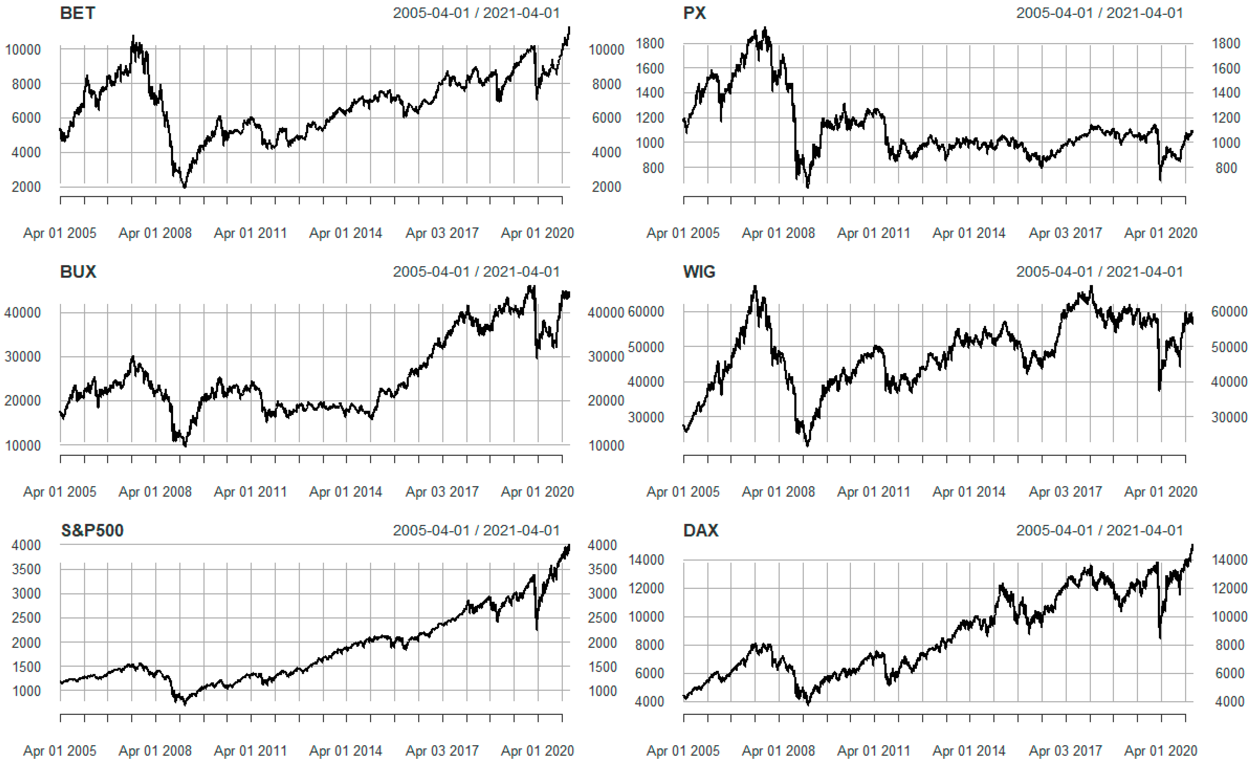
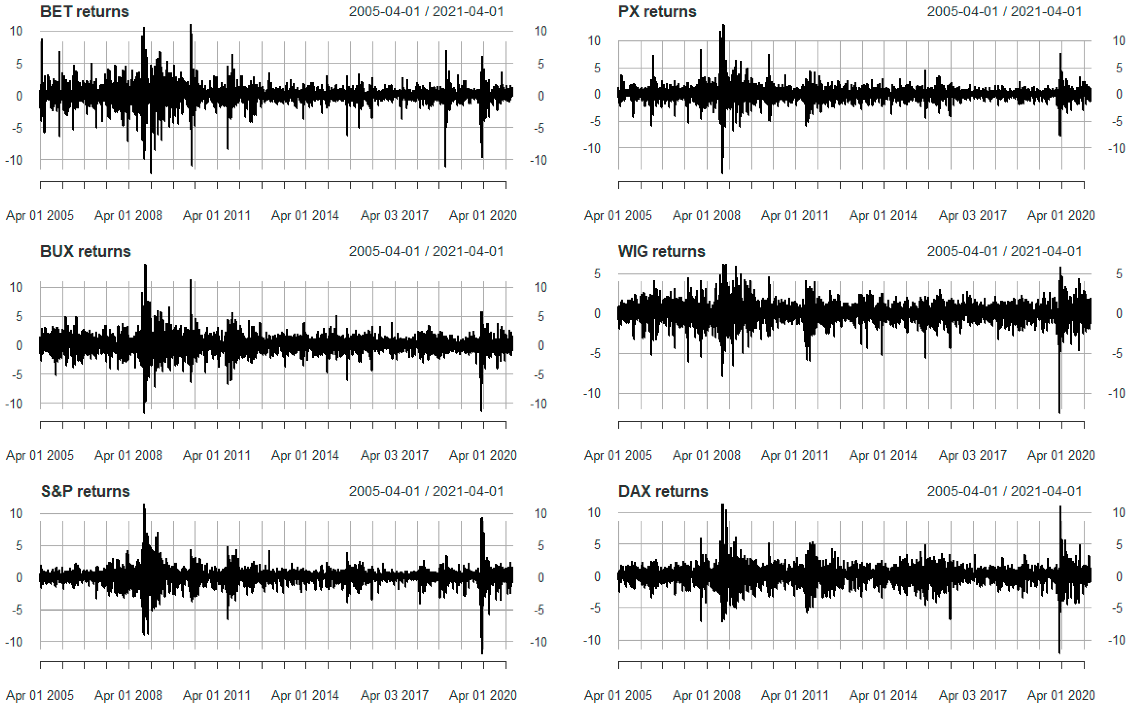
where $r_t={\left(r_{1,t},r_{2,t},\dots ,r_{n,t}\right)}^{\prime }$, ${\epsilon }_t={\left({\epsilon }_{1,t},{\epsilon }_{2,t},\dots ,{\epsilon }_{n,t}\right)}^{\prime }$ and ${\epsilon }_t|I_{t-1}~N\left(0,H\right)$. $r_t$ is a (n × 1) vector of stock market returns and ε_t is a (n × 1) vector of conditional residuals. In this study, the vector r_t consists of the returns on the four CEEC stock indices (BET, PX, BUX, WIG), as well as the rates of return on stock indices from the two developed countries considered (S&P500 and DAX). We initially considered both developed markets (US and German markets) with one day delay.

Potential motivation for the inclusion of the developed stock markets in the mean equation is that they serve as global (US) and regional (Germany) factors, playing a crucial role in determining the rates of return on stock indices from Central and Eastern Europe, [6] (Chiang et al., 2007).

Within the analysis, we have also incorporated the different time zones (Drożdż et al., 2001 [60]) in which the European and the US stock markets are traded, additionally estimating a new DCC-GARCH model for DAX index without delay.

The conditional variance–covariance matrix is further specified as follows:

$$H_t=D_t{R}_t{D}_t$$

(2)

where $D_t$ is a diagonal matrix of size (n × n), which contains time-varying standard deviations that are obtained from univariate GARCH models. $D_t$ presents the terms $\sqrt{h_{ii,t}}$ on the ith diagonal, i = 1, 2, …, n (The univariate GARCH(1,1) model is specified as: $h_{ii,t}={\omega }_i+{\alpha }_{i,1}{\epsilon }_{i,t-1}^2+{\beta }_{i,1}{h}_{ii,t-1}$, for i = 1, 2, …, n), and $R_t$ is the time-varying correlation matrix of size (n × n).

The DCC-GARCH model proposed by [61] Engle and Sheppard (2002) involve two stages of estimation of the conditional variance–covariance matrix $H_t$:

-

in the first stage, univariate volatility models are fitted for each rate of return and estimates for $\sqrt{h_{ii,t}}$ are obtained.

-

in the second stage, stock return residuals are transformed by their estimated standard deviations, (obtained in the first stage), as follows: $u_{i,t}={\epsilon }_{i,t}/\sqrt{h_{ii,t}}$, then $u_{i,t}$ is used to estimate the parameters of the conditional correlation.

The expression gives the evolution of the correlation in the DCC-GARCH model:

$$Q_t=\left(1-a-b\right)Q+a{u}_{t-1}{u}_{t-1}{}^{\prime }+b{Q}_{t-1}$$

(3)

where $Q_t=\left(q_{ij,t}\right)$ is the (n × n) time-varying variance–covariance matrix of $u_t$, $Q=\overline{E}\left[u_t{u}_t{}^{\prime }\right]$ is the (n × n) unconditional variance–covariance matrix of $u_t$, while $a \mathrm{and} b$ are non-negative scalar parameters that satisfy the expression $\left(a+b\right)<1$. (A typical element of $Q_t$ is: $q_{ij,t}=\left(1-a-b\right){\rho }_{ij}+a{u}_{i,t-1}{u}_{j,t-1}{}^{\prime }+b{q}_{ij,t-1}$, where ${\rho }_{ij}$ represents the unconditional correlations of $u_{i,t}{u}_{j,t}$).

Because the matrix $Q_t$ is a variance–covariance matrix, it generally does not have the value 1 on the diagonal; therefore, it is adjusted to obtain an appropriate correlation matrix $R_t$. Thus:

$$R_t={\left(Q_t^{*}\right)}^{-1}{Q}_t {\left(Q_t^{*}\right)}^{-1}$$

(4)

where $Q_t^{*}$ is a diagonal matrix containing the elements $\sqrt{q_{ii,t}}$ … $\sqrt{q_{nn,t}}$. Matrix $Q_t^{*}$ resizes the items in the $Q_t$ matrix, so that $|{\rho }_{ij,t}\left|=\right|\frac{q_{ij,t}}{\sqrt{q_{ii,t}{q}_{jj,t}}}|$ $\le$ 1.

Now $R_t$ from Equation (4) is a correlation matrix with the value 1 on the diagonal and off-diagonal elements smaller than 1 in absolute value, if $Q_t$ is positively definite.

$${\rho }_{ij,t}=q_{ij,t}/\sqrt{q_{ii,t}{q}_{jj,t}}, i,j=1,2\dots \dots .., n and i\ne j$$

(5)

5.2. Empirical Results and Discussions

In the first stage of the model, the volatilities of the returns on the four CEEC stock market indices were analyzed through univariate GARCH models, which highlighted, for all series, a first-order autoregressive structure, AR (1). This shows that the stock returns from the previous day significantly influence the returns of the current day. The empirical results unanimously reveal that the GARCH (1,1) model is optimal for all stock indices.

In the second phase of the analysis, the dynamic structure of the four emerging stock markets and the potential contagion effect from the two developed markets were explored. This was achieved by estimating two DCC-GARCH models in which S&P500 and DAX function as exogenous variables.

The results of the multivariate DCC-GARCH models are presented in

Table 1. Estimation results from the DCC-GARCH models (CEEC-USA).

	BET	PX	BUX	WIG	S&P500t−1
Panel A: Mean equations
µ	0.079 ***	0.029 **	0.052 ***	0.028 **	0.07 ***
${\gamma }_1$	0.044 **	−0.090 ***	−0.024	−0.035 *	−0.035
${\gamma }_2$	0.152 ***	0.280 ***	0.220 ***	0.240 ***	-
Panel B: Variance equations
Ω	0.053 ***	0.022 ***	0.037 ***	0.019 ***	0.029 ***
${\alpha }_i$	0.204 ***	0.145 ***	0.097 ***	0.069 ***	0.138 ***
βi	0.788 ***	0.851 ***	0.884 ***	0.916 ***	0.840 ***
Persistence	0.992	0.996	0.981	0.985	0.978
Panel C: DCC equation
a	0.012 ***
b	0.967 ***

Note: ***, **, * means statistically significant at the 1%, 5% and 10% levels, respectively.

and

Table 2. Estimation results from the DCC-GARCH models (CEEC-Germany).

	BET	PX	BUX	WIG	DAXt−1
Panel A: Mean equations
µ	0.081 ***	0.036 ***	0.062 ***	0.042 ***	0.089 ***
${\gamma }_1$	0.047 ***	0.055 ***	0.006 *	0.035 *	0.042
${\gamma }_2$	0.052 ***	0.117 ***	0.057 **	0.036 **	-
Panel B: Variance equations
Ω	0.044 ***	0.024 ***	0.037 ***	0.019 ***	0.029 ***
${\alpha }_i$	0.200 ***	0.143 ***	0.095 ***	0.069 ***	0.095 ***
${\beta }_i$	0.797 ***	0.846 ***	0.886 ***	0.917 ***	0.887 ***
Persistence	0.997	0.989	0.981	0.986	0.982
Panel C: DCC equation
a	0.014 ***
b	0.967 ***

Note: ***, **, * means statistically significant at the 1%, 5% and 10% levels, respectively.

. The models were run, one at a time, for each stock return on the four CEEC indices, first with the returns on the S&P500 index (as a global exogenous factor), and subsequently with the returns on the DAX index (as a regional exogenous factor).

Each table contains three sections, presenting the estimates of the coefficients from the following equations:

• Panel A: Mean equation

  $$\begin{gathered} r_t=\mu +{\gamma }_1{r}_{t-1}+{\gamma }_2{r}_{t-1}^{USA,DE }{\epsilon }_t, \\ {r}_t={\left(r_{1,t},r_{2,t},\dots ,r_{5,t}\right)}^{\prime } {\epsilon }_t={\left({\epsilon }_{1,t},{\epsilon }_{2,t},\dots ,{\epsilon }_{5,t}\right)}^{\prime } \mathrm{and} {\epsilon }_t|I_{t-1}~N\left(0,H\right) \end{gathered}$$
• Panel B: Variance equation:

  $$h_{ii,t}={\omega }_i+{\alpha }_{i,1}{\epsilon }_{i,t-1}^2+{\beta }_{i,1}{h}_{ii,t-1}, \mathrm{for} i = 1.2,\dots ,5$$
• Panel C: DCC equation:

  $$\begin{gathered} q_{ij,t}=\left(1-a-b\right){\rho }_{ij}+a{u}_{i,t-1}{u}_{j,t-1}{}^{\prime }+b{q}_{ij,t-1} \\ {\rho }_{ij,t}=q_{ij,t}/\sqrt{q_{ii,t}{q}_{jj,t}}, where i,j=1,2\dots ,5, and i\ne j \end{gathered}$$

Panel A, from both tables, indicates that the intercept in the mean equation (Equation (1)) is statistically significant for all stock markets, while the term AR (1), ${\gamma }_1$, is statistically significant and negative for the Czech Republic and Poland and statistically significant and positive for Romania.

In Table 1, the influence of the US stock market over the markets from the CEEC is highlighted by the term ${\gamma }_2$, which is statistically significant for all Central and Eastern European stock markets at the 1% level. In Table 2, the same coefficient is also significant at the 5% level, suggesting that the DAX index also influences the stock markets in Romania, the Czech Republic, Hungary, and Poland. These results are consistent with those in the literature [6] (Chiang et al., 2007), which argue that the US and Germany play an important role in the evolution of emerging markets at both the global and regional level; in this case, the influence is observed on the stock markets in Central and Eastern Europe. Similar results have been obtained by [11] Grabowski (2019), highlighting the significant impact of the US stock market on the euro area and transition countries.

Panel B contains the estimators in the variance equation. The coefficients ${\alpha }_i$ (of the ARCH term—${\epsilon }_{i,t-1}^2$) and ${\beta }_i$ (of the GARCH term—$h_{ii,t-1}$) are statistically significant, justifying the use of the GARCH (1,1) model to capture the contagion effect in the analyzed markets. Furthermore, the persistence of volatility, measured by the sum of the coefficients ${\alpha }_i$ and ${\beta }_i$, is very close to 1 for all the stock markets examined. This indicates that volatility in the GARCH models is highly persistent.

The two rows in panel C represent the estimators of the DCC (1,1) parameters, a and b. Both parameters are statistically significant in correlation with the S&P500 and the DAX indices, revealing a substantial co-movement that varies over time between these stock returns. Furthermore, the conditional correlation coefficients also show high persistence, with the sum of the two coefficients (a + b) being more than 0.90 during the period considered.

We also tested the implications of different time zones in which the European and the US stock markets are traded, building a new DCCC-GARCH model that considers the German market as a benchmark and where the returns on the DAX index are considered as a regional exogenous factor (

Table 3. Estimation results from the DCC-GARCH models (CEEC-Germany).

	BET	PX	BUX	WIG	DAX
Panel A: Mean equations
µ	0.070 ***	0.005	0.029 *	0.005	0.090 ***
${\gamma }_1$	0.044 ***	0.059 ***	0.004 **	0.024 **	0.045 *
${\gamma }_2$	0.244 ***	0.448**	0.523 ***	0.524 **	-
Panel B: Variance equations
Ω	0.044 **	0.022 ***	0.024 ***	0.014 ***	0.029 ***
${\alpha }_i$	0.203 ***	0.113 ***	0.068 ***	0.070 ***	0.096 ***
${\beta }_i$	0.790 ***	0.864 ***	0.914 ***	0.913 ***	0.887 ***
Persistence	0.993	0.977	0.982	0.983	0.982
Panel C: DCC equation
a	0.045 **
b	0.987 ***

Note: ***, **, * means statistically significant at the 1%, 5% and 10% levels, respectively.

.).

In each table, Panel A indicates that the intercept in the mean equation (Equation (1)) is statistically significant for all stock markets, while the term AR (1), γ₁, is statistically significant and negative for the Czech Republic and Poland and statistically significant and positive for Romania. In Table 3, the influence of the German stock market over the markets from the CEEC is highlighted by the term γ₂, which is statistically significant for all Central and Eastern European stock markets at the 5% level, suggesting that the DAX index influences, as well, the stock markets in Romania, the Czech Republic, Hungary and Poland. These results are consistent with those in the literature [8] (Chiang et al., 2007), which argue that the US and Germany play an important role at the global and regional levels.

In Panel B, which contains the estimators in the variance equation, the coefficients α_i are statistically significant, justifying the use of the GARCH (1,1) model to capture the contagion effect in the analyzed markets. Furthermore, the persistence of volatility, measured by the sum of the coefficients α_i and β_i, is very close to 1 for all the stock markets examined. This indicates that volatility in the GARCH models is highly persistent. The two rows in panel C represent the estimators of the DCC (1,1) parameters, a and b. Furthermore, the conditional correlation coefficients also show high persistence, with the sum of the two coefficients (a + b) being more than 0.90 during the period considered.

One of the most essential advantages of the DCC-GARCH model is obtaining all the possible correlations between the examined variables, allowing for study of coefficient behavior during periods of particular interest, such as economic crises.

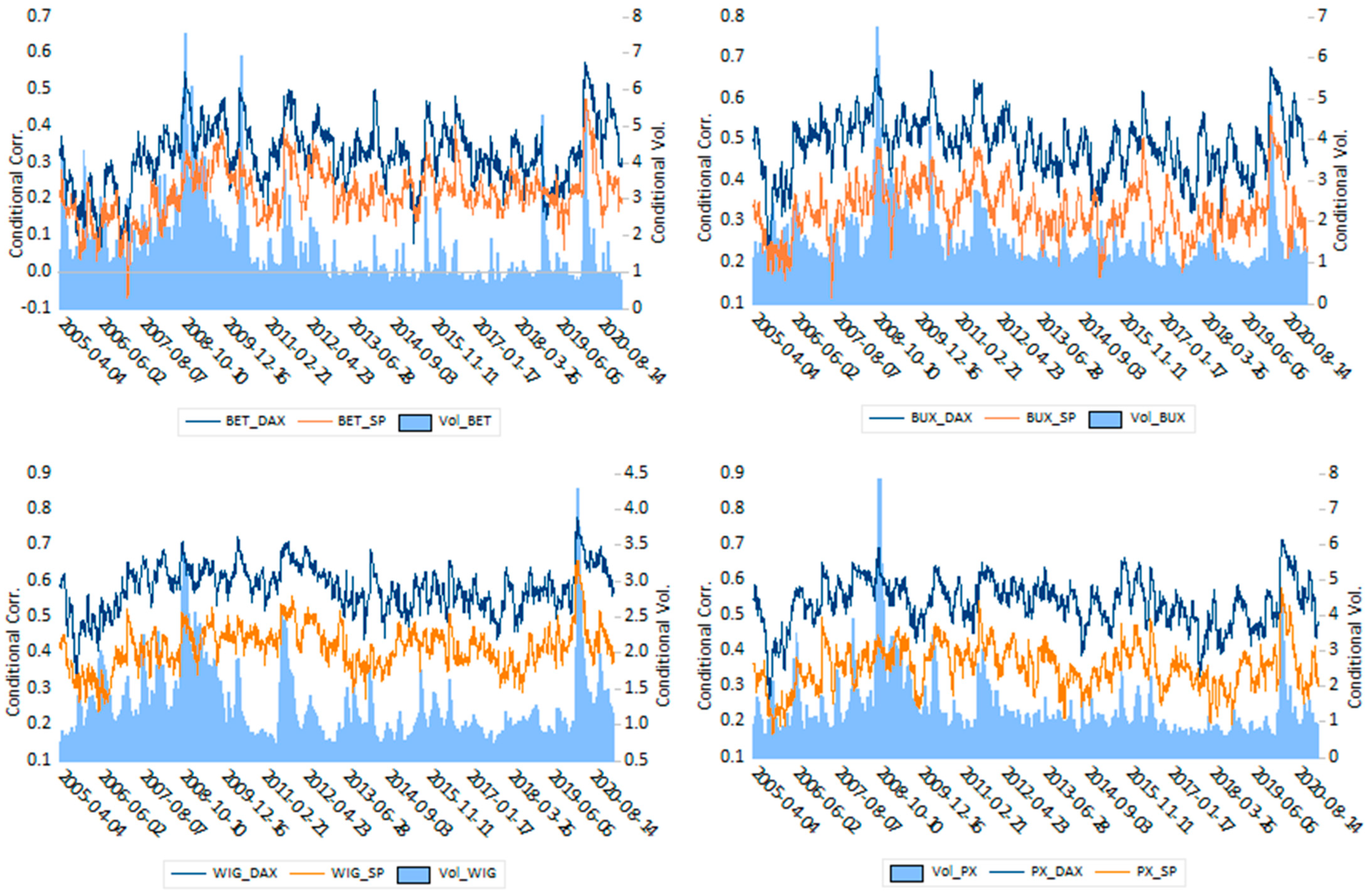
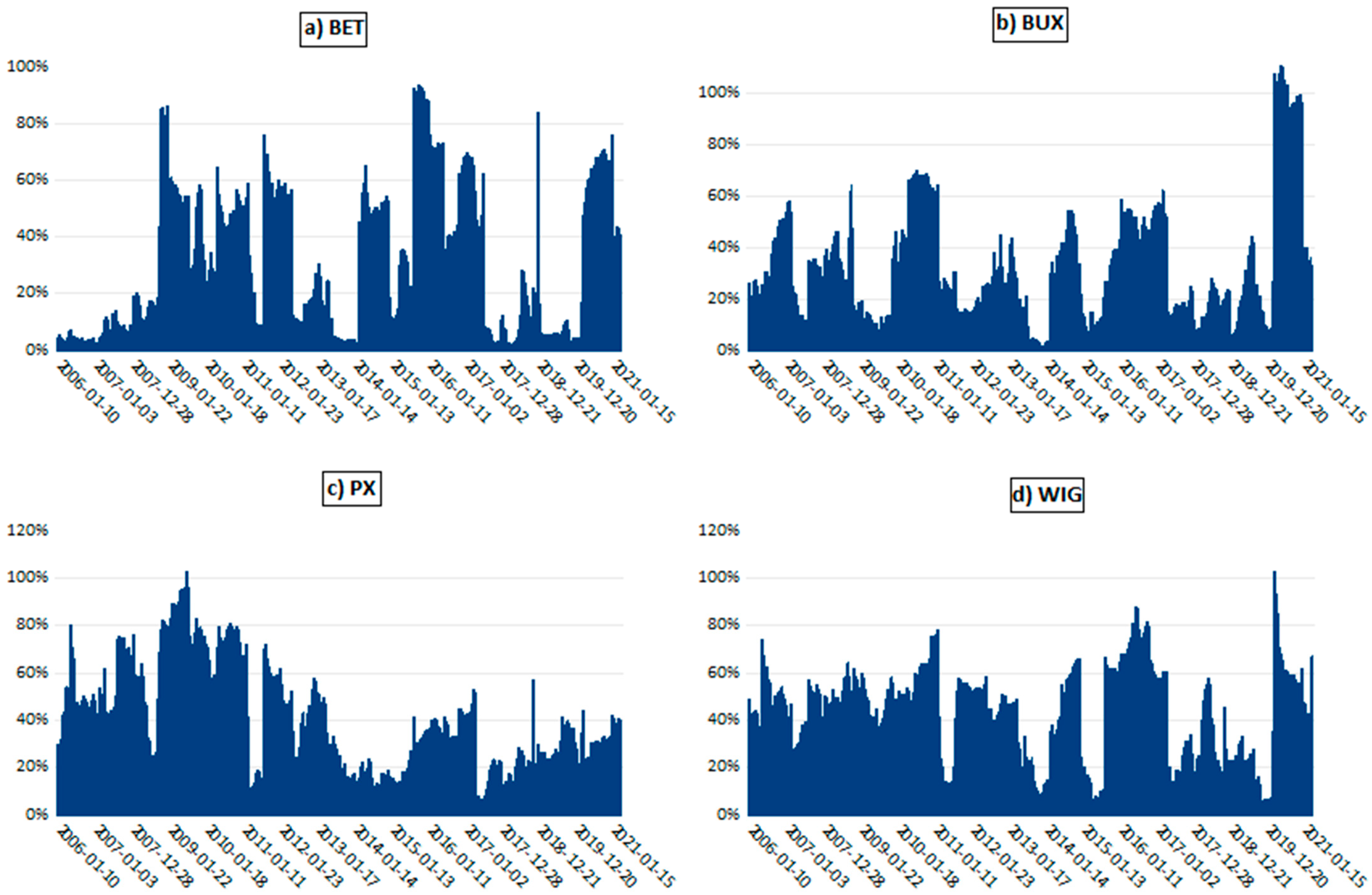
Therefore, the conditional correlation coefficients between the four CEEC stock indices and the S&P500 index, followed by the DAX index, were estimated, their graphic representations are shown in Figure 2 and Figure 3. In both models, we have considered one day delay for both markets (US and German). In Appendix G, for each CEEC index, conditional correlations are presented along with the conditional volatilities, which were calculated in the first stage of the DCC-GARCH model.

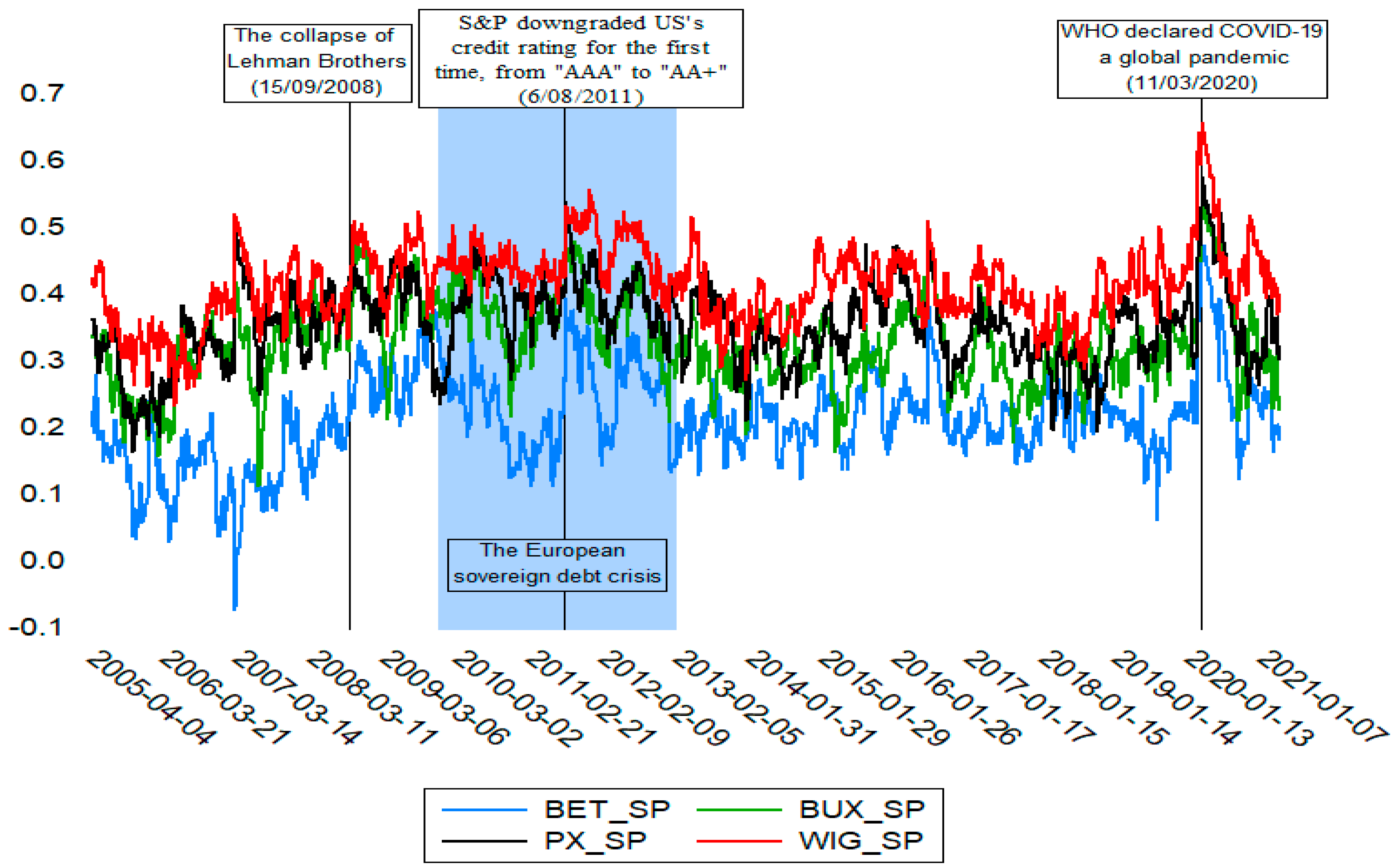
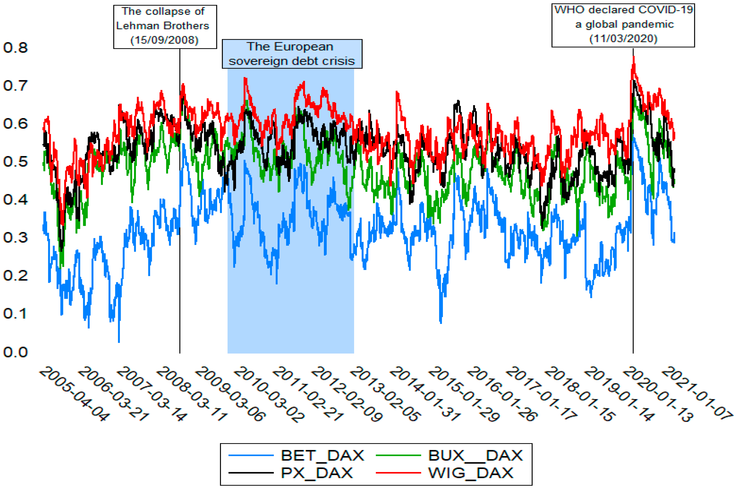
Figure 2 and Figure 3 show that the stock markets in Central and Eastern Europe generally have a higher conditional correlation with the DAX index than with the S&P500 index.

Poland and the Czech Republic, as counties that neighbor Germany, register the most significant correlations with it. Therefore, these markets are very sensitive to fluctuations in stock market returns in Germany. Grabowski (2019) [11] and Bein and Tuna (2015) [52] also acknowledged the higher conditional correlation of the Polish and Czech stock markets with Germany and the US compared to Hungary.

Compared to the CEE-4 nations, conditional correlations for developed markets are greater and follow different patterns. Poland, the Czech Republic, Romania, and Hungary’s stock markets had a weak integration with those of developed countries during 2005 and 2006. The more rapid response of the Prague stock market to shocks coming from developed countries soon after the EU’s admission is consistent with the findings of the paper by [62] Savva and Aslanidis (2010). Following EU accession, there is an increase in the correlations between CEE countries and developed stock markets, confirmed by [63] Deltuvaite (2016). During the euro area sovereign debt crisis, the stock markets in the CEE-4 nations showed themselves to be very susceptible to foreign shocks ([11] Grabowski, 2019).

The above aspect is captured both in Figure 3 and in

Table 4. The average conditional correlation coefficient and the volume of trade (exports and imports) between CEEC countries and Germany and the US (2020).

	Romania	Czech Republic	Hungary	Poland
Avg. Rho Germany	0.33	0.54	0.49	0.59
Avg. Rho US	0.21	0.35	0.32	0.41
The volume of exports to Germany (bn. USD)	16.19	62.79	33.38	73.51
% of the country’s exports	23%	33%	28%	29%
The volume of imports from Germany (bn. USD)	19.17	39.68	27.88	55.80
% of the country’s imports	21%	24%	25%	22%
% of Germany’s total imports	1.4%	4.4%	2.8%	5.9%
% of Germany’s total exports	1.3%	3.3%	2.1%	5.4%

, where the average correlation coefficient (Avg. Rho) is presented.

The influence of the German stock market on the analyzed CEEC stock markets is also because Germany is the leading trading partner of these countries, given the volume of imports and exports shown in Table 3.

Table 4 suggests that the benefits of diversification for investors who own shares in mature markets such as Germany and those in CEEC markets may be limited, with PX, BUX, and WIG recording average correlations between 0.49 and 0.59 with DAX. In the case of the BET index, the average correlation coefficient with the German stock index is lower, 0.33. As shown in Table 3, Romania has the lowest volume of exports/imports with Germany, approximately 1.3% of Germany’s total trade.

When there is correlation with both the DAX index and the S&P500 index, the coefficients increased significantly during turbulent periods, such as those identified in Figure 2 and Figure 3 above. For all CEEC countries, the maximum correlation coefficient was reached in March 2020, when COVID-19 was officially declared a global pandemic by the World Health Organization (WHO). This major event, which had affected the year even prior to the pandemic declaration, has had devastating effects on all sectors of activity because governments decided to restrict movement and limit economic activities to protect the population and slow down the spread of the virus. Under these strict mobility measures, exports and imports between trading partners have decreased significantly. Empirical evidence supporting these results has also been shown by [64] Papathanasiou et al. (2022), highlighting that during 2020–2021, the level of volatility spillovers has been moderate, while [42] Samitas et al. (2022) demonstrated the volatility spillovers between natural alternative instruments and a set of traditional high-demand instruments, revealing the integration of markets and total connectedness during stress periods. During this period, the highest coefficients of conditional correlation were recorded in the case of Poland, reaching values of around 0.8 with Germany and 0.7 with the US.

Over the entire period examined, the Polish index, WIG, was the most correlated with DAX and S&P500 indices compared to the other stock indices analyzed in Central and Eastern Europe. The BET index, meanwhile, is the least correlated with these two benchmark stock indices.

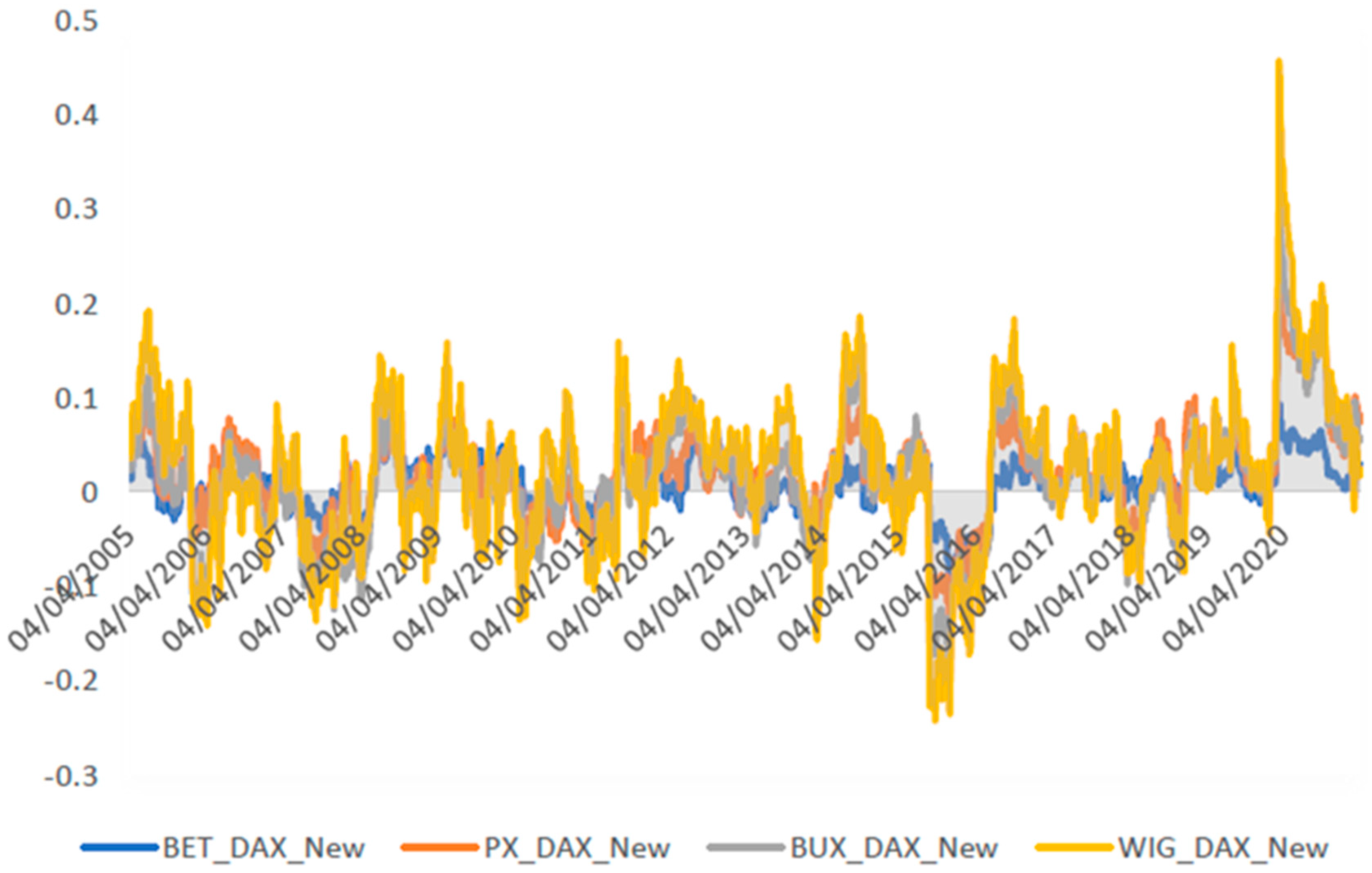
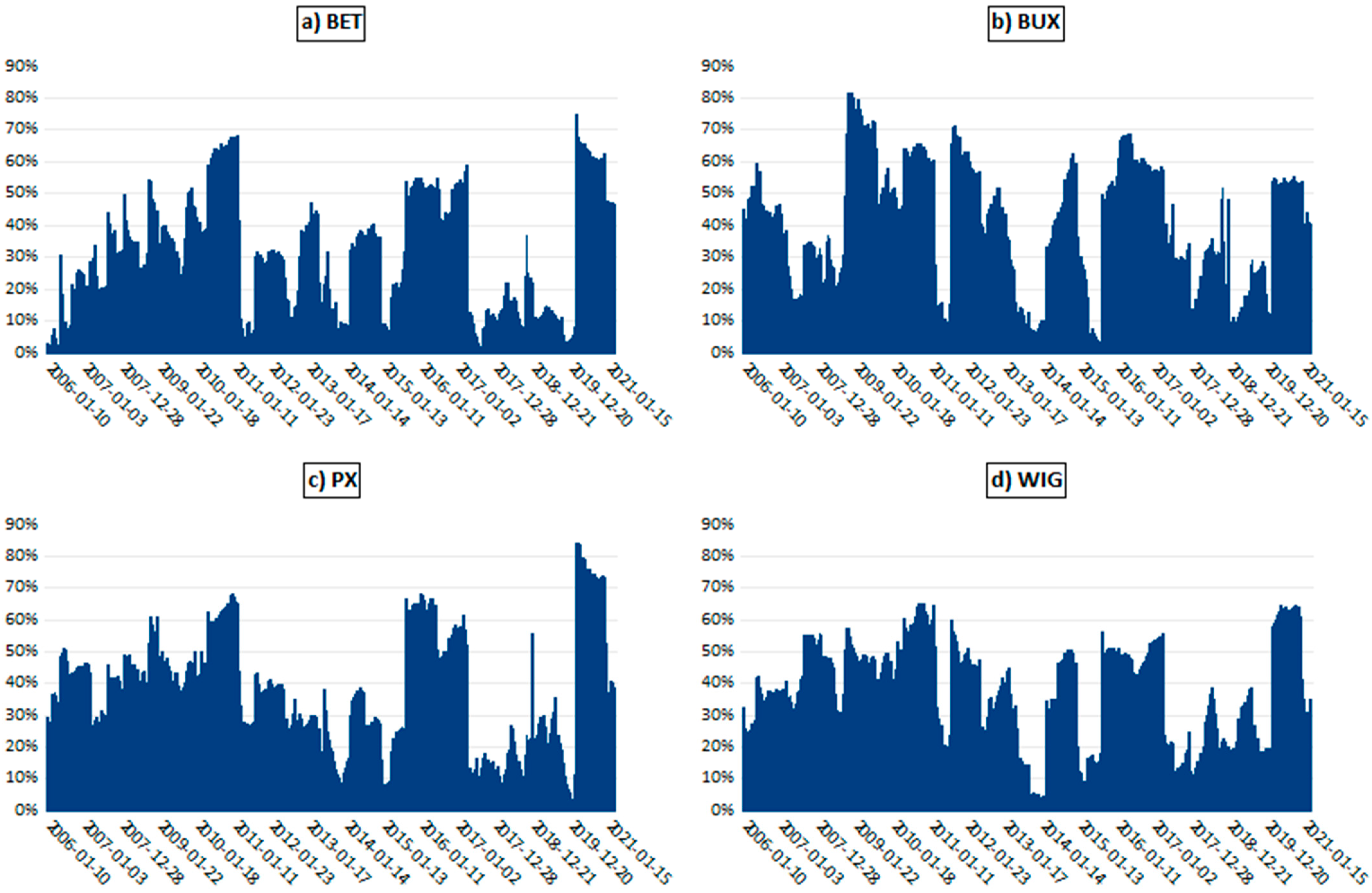
However, the results seem to be quite different when the European and the US stock markets are traded in different time zones, considering first the European and then American one day later. Analyzing now, the conditional correlation coefficients between the four CEEC stock indices and the DAX index in both cases (with and without delay) presented in Figure 3 and Figure 4 revealed a visible drop in the correlations when the German market was considered without delay.

Comparing these new conditional correlations of four European markets in relation to DAX with those concerning the US market but with one day delay (Figure 2 and Figure 4), it is worth mentioning that the stock markets in Central and Eastern Europe tend to have a higher conditional correlation with the S&P 500 index than with the DAX index.

Therefore, the different time zones in which the European and US stock markets trade are incorporated within the research; the main conclusion leads to the general idea, as in the case of [60] Drożdż et al., that the US market dictates the trend.

The results are also in line with the study of [10] Horváth et al.(2017), demonstrating that financial contagion occurred between 1998 and 2014. Kang and Lee (2019) [65] showed that the UK and US futures index markets are the most important contributors of the volatility spillover shock of the global futures markets.

Analyzing the spillover effects between US stock, crude oil, and gold markets from 2006 through 2019, [66] Bouri et al. (2021) proved that the stock index is the main net transmitter, oil is the main net transmitter, and gold is a net receiver.

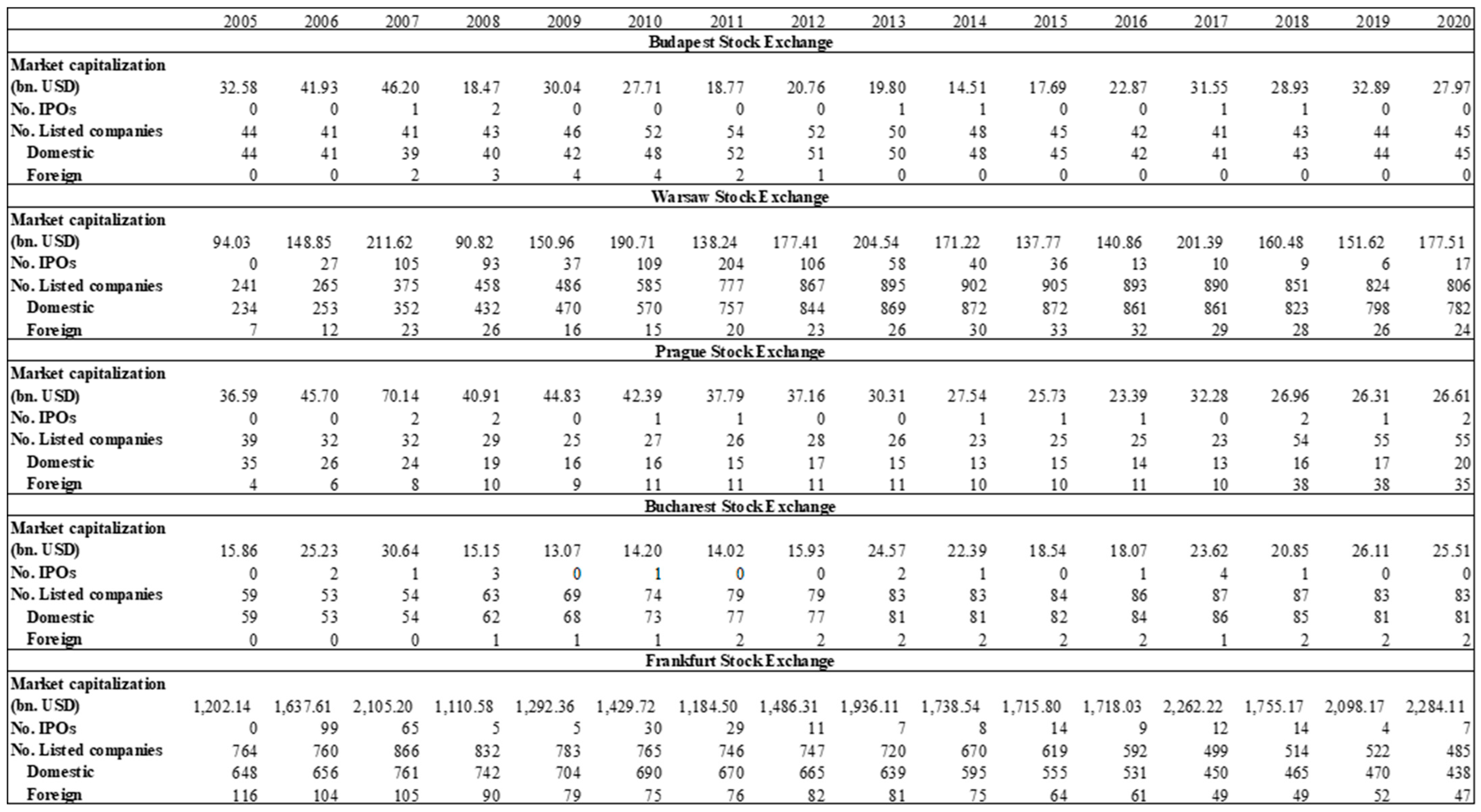
The Warsaw Stock Exchange is the largest in the CEEC area. At the end of 2020, the WSE had 806 listed companies and a market capitalization of approximately 178 billion USD, while the remaining CEEC stock markets registered below 100 listed companies and a market capitalization between 25–28 billion USD. Furthermore, Poland is the only country in this group that was promoted from emerging to developed market status by Financial Times Stock Exchange Russell (FTSE Russell), a global index and financial rating provider.

According to the FTSE Russell classification, global capital markets fall into three broad categories: developed, emerging, and frontier markets. These are determined according to several essential criteria: economic development, size, liquidity, and accessibility.

The Prague Stock Exchange and the Budapest Stock Exchange were classified as emerging markets before 2008. In September 2020, the Bucharest Stock Exchange was moved from frontier market to emerging market status in the FTSE Russell indices. The promotion of the Bucharest Stock Exchange will attract substantial funds to listed companies (which was not previously possible because of restrictions generated by the Frontier market status), and implicitly, to the development of the Romanian economy.

The existing literature argues that the contagion phenomenon in the financial markets can be induced in two ways: interdependencies between markets or investor behavior. The concept of interdependence was discussed by [4] Forbes and Rigobon (2002); it represented the spread of shocks from one financial market to another, leading to a significant increase in the correlation in these markets. According to the article written by [3] Dornbusch, Park, and Claessens (2000), however, the increase in correlation between financial markets during periods of crisis could also be attributed to contagion caused by the herding behavior of investors. Investors follow the behavior of other market participants, thus trading in the same direction over a certain period. Several studies in the literature (including [6] Chiang, Jeon, and Li (2007); [8] Syllignakis and Kouretas (2011)) use models such as the DCC-GARCH model to investigate possible herding behavior in emerging financial markets during turbulent periods.

5.3. Quantification of the Contagion Effect in Times of Crisis—Analysis Based on DUMMY Variables

The behavior of the conditional correlation coefficients over time has been further studied, providing insight into the impact that periods of crisis have on the evolution of these correlations. Specifically, 3 DUMMY variables were used to capture the dynamics of the conditional correlation coefficients for different periods of crisis.

Therefore, the regression model used is given by the following expression:

$${\rho }_{ij,t}=\omega +{\displaystyle \sum }_{p=1}^N{\varnothing }_p{\rho }_{ij,t-p}+{\displaystyle \sum }_{k=1}^2{\alpha }_{k}D{M}_k+{\alpha }_{3}D{M}_3^i+e_{ij,t}$$

(6)

where ${\rho }_{ij,t}$ is the dynamic correlation coefficient between the US and Germany and the four CEEC countries analyzed ($i$ = US, Germany; $j$ = Romania, Czech Republic, Poland, and Hungary). The DUMMY variable $D{M}_3^i$ was selected to represent the period of the SARS-CoV-2 pandemic, and two different time frames were chosen for the correlation with the S&P500 index and the DAX index, as the pandemic affected the economies differently depending on the degree of spread of the virus.

The lag order in Equation (6) was selected through the analysis of the correlograms and the Akaike information criterion (AIC), with lag 1 being selected for all equations.

Table 5. Dynamic conditional correlation coefficients during periods of crisis.

	Romania	Czech Republic	Hungary	Poland
	BET	PX	BUX	WIG
CEEC—USA
$\omega$	0.0050 ***	0.0085 ***	0.0073 ***	0.0104 ***
${\rho }_{t-1}$	0.9751 ***	0.9750 ***	0.9766 ***	0.9742 ***
$D{M}_{1,t}$	0.0022 **	0.0016 **	0.0021 **	0.0019 **
$D{M}_{2,t}$	0.0039 **	0.0028 *	0.0031 **	0.0035 **
$D{M}_{3,t}^{USA}$	0.0042 ***	0.0044 ***	0.0044 ***	0.0032 ***
CEEC—GE
$\omega$	0.0054 ***	0.0086 ***	0.0077 ***	0.0111 ***
${\rho }_{t-1}$	0.9818 ***	0.9833 ***	0.9837 ***	0.9804 ***
$D{M}_{1,t}$	0.0020 **	0.0008	0.0011	0.0014 **
$D{M}_{2,t}$	0.0043 **	0.0031 **	0.0018	0.0032 **
$D{M}_{3,t}^{GE}$	0.0032 ***	0.0020 ***	0.0021 **	0.0023 ***

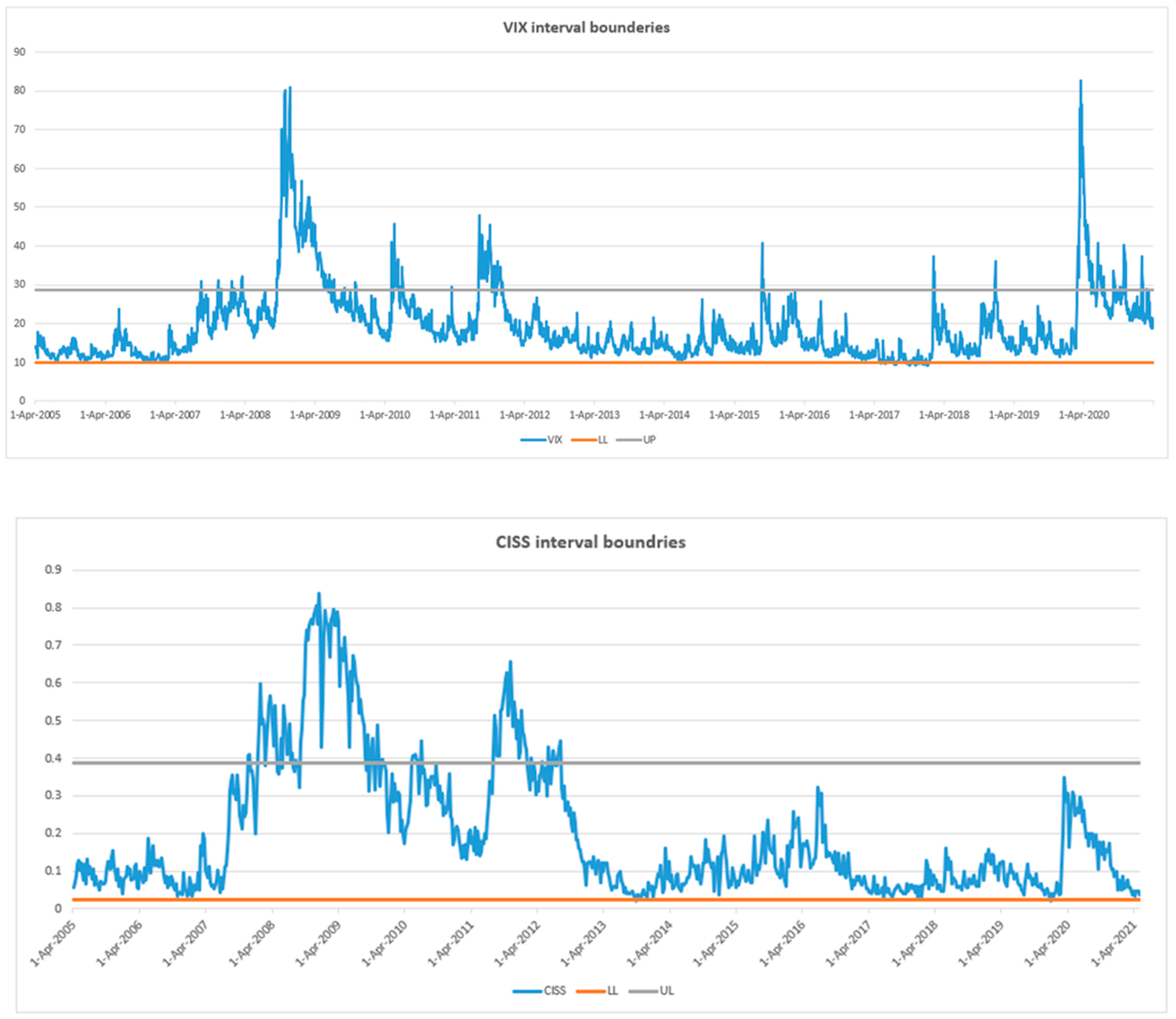
Note: ***, **, * means statistically significant at the 1%, 5% and 10% levels, respectively.

presents the estimates of the regression model described above. Economic events with a major impact on stock markets were used to establish the crisis periods, as well as the VIX index (also used by [13] Beirne John et al. (2013)) and the Composite Indicator of Systemic Stress (CISS) calculated by the ECB for the eurozone. The VIX Index is calculated by the Chicago Board Options Exchange (CBOE), based on the prices of options on the S&P500 index, thus measuring the stock market’s volatility over the following 30 days. Appendix H presents the evolution of the VIX and the CISS indices, respectively, with turbulent periods captured by the threshold defined at a standard deviation above the average.

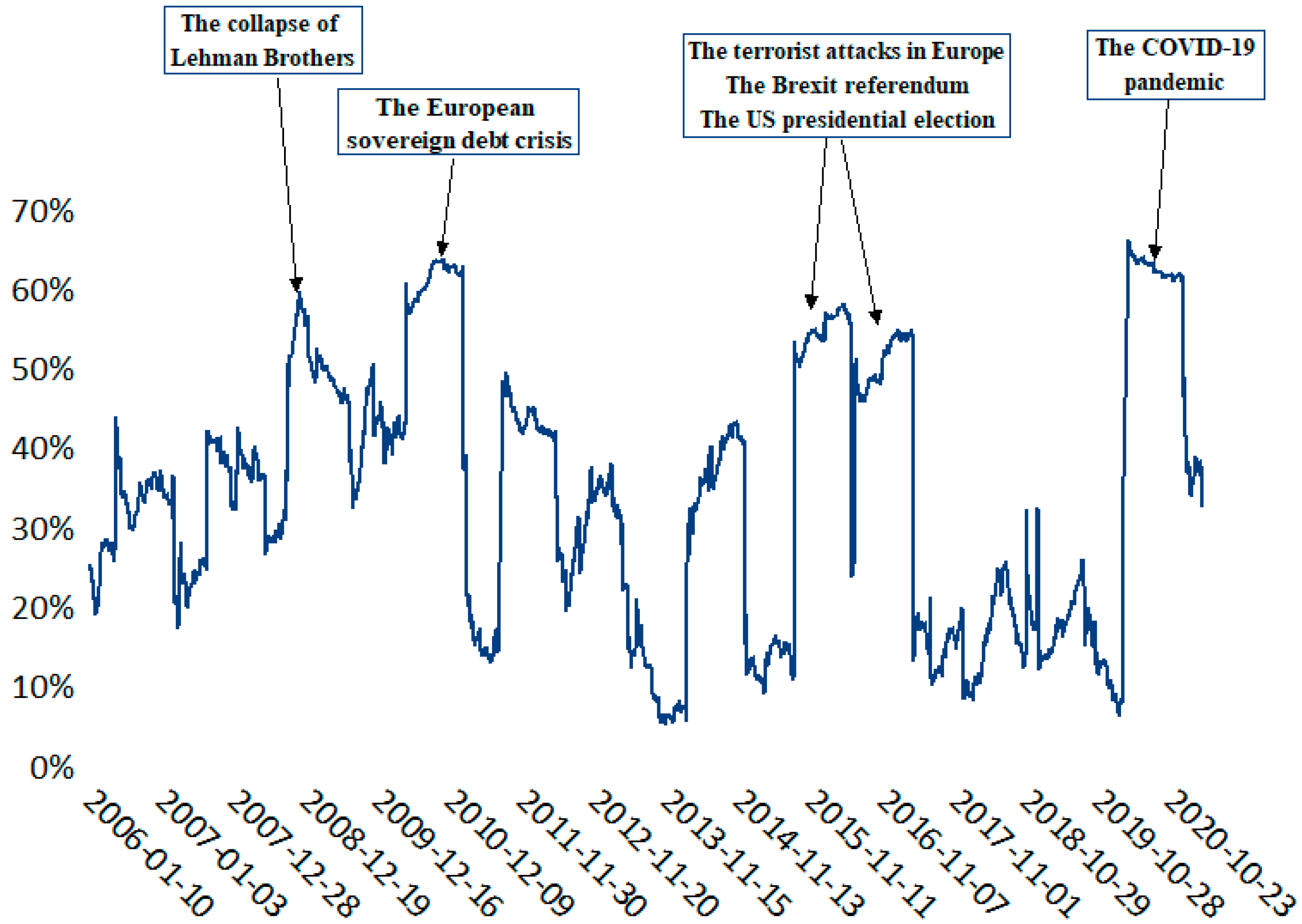
The first analysis of the dynamics of correlation coefficients refers to the period of the Great Recession, with the first DUMMY variable $D{M}_1$ taking the value 1 between 15 September 2008–31 July 2009 and 0 otherwise. This turbulent period began with the bankruptcy of Lehman Brothers, the selection of the interval being also based on the analysis of the volatility of the VIX index and that of the CISS index.

Although the premises of this crisis have been the same since the end of 2007, the Great Recession was triggered by the bankruptcy of the largest American investment bank, Lehman Brothers, on 15 September 2008; the crisis then spread globally. Worldwide stock markets collapsed, the Dow Jones and the S&P500 indices recording major “intraday” declines of 6.98% and 8.8%, respectively, on 29 September 2008 (after the US Congress rejected the $700 billion financial aid plan).

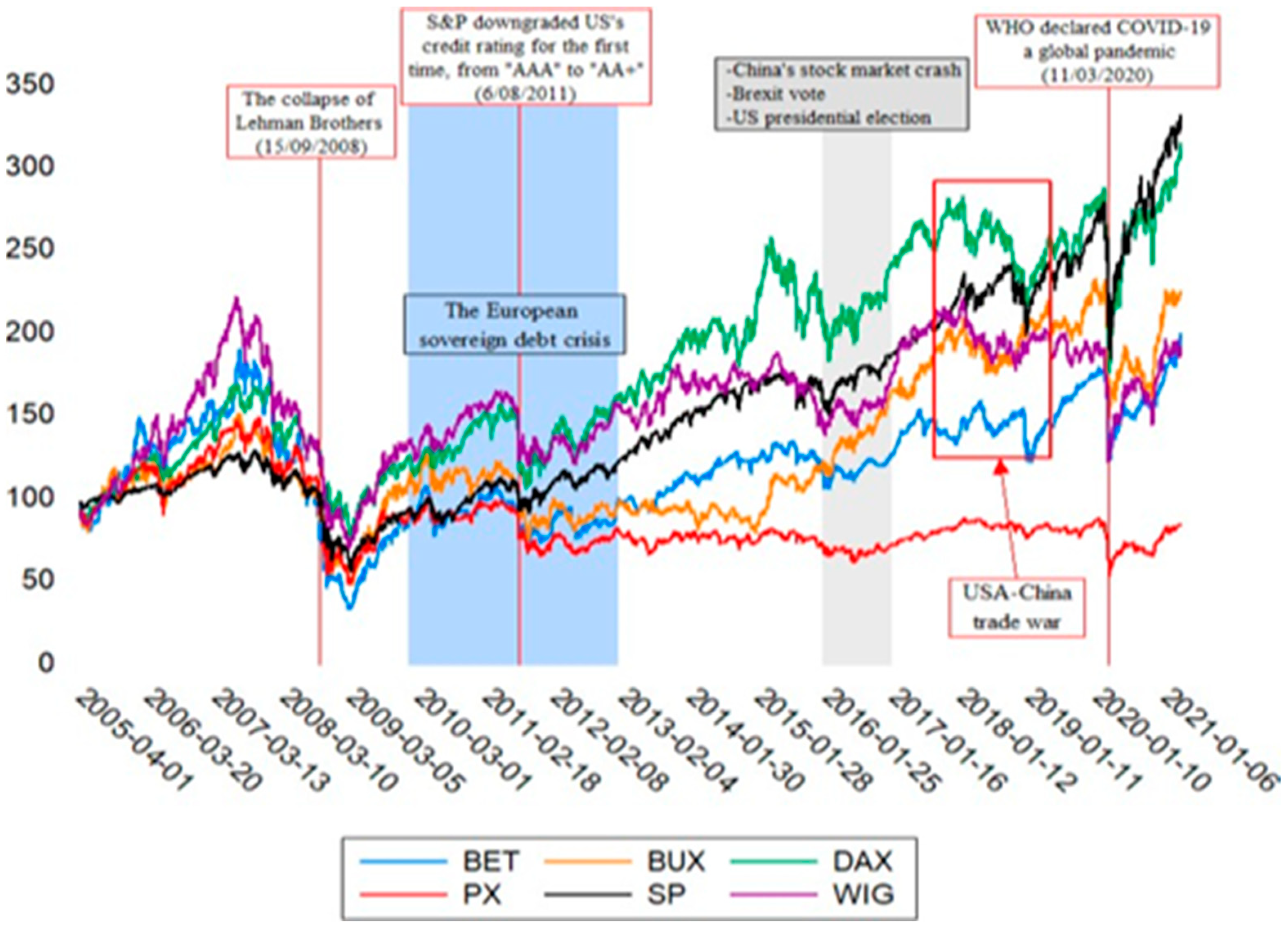
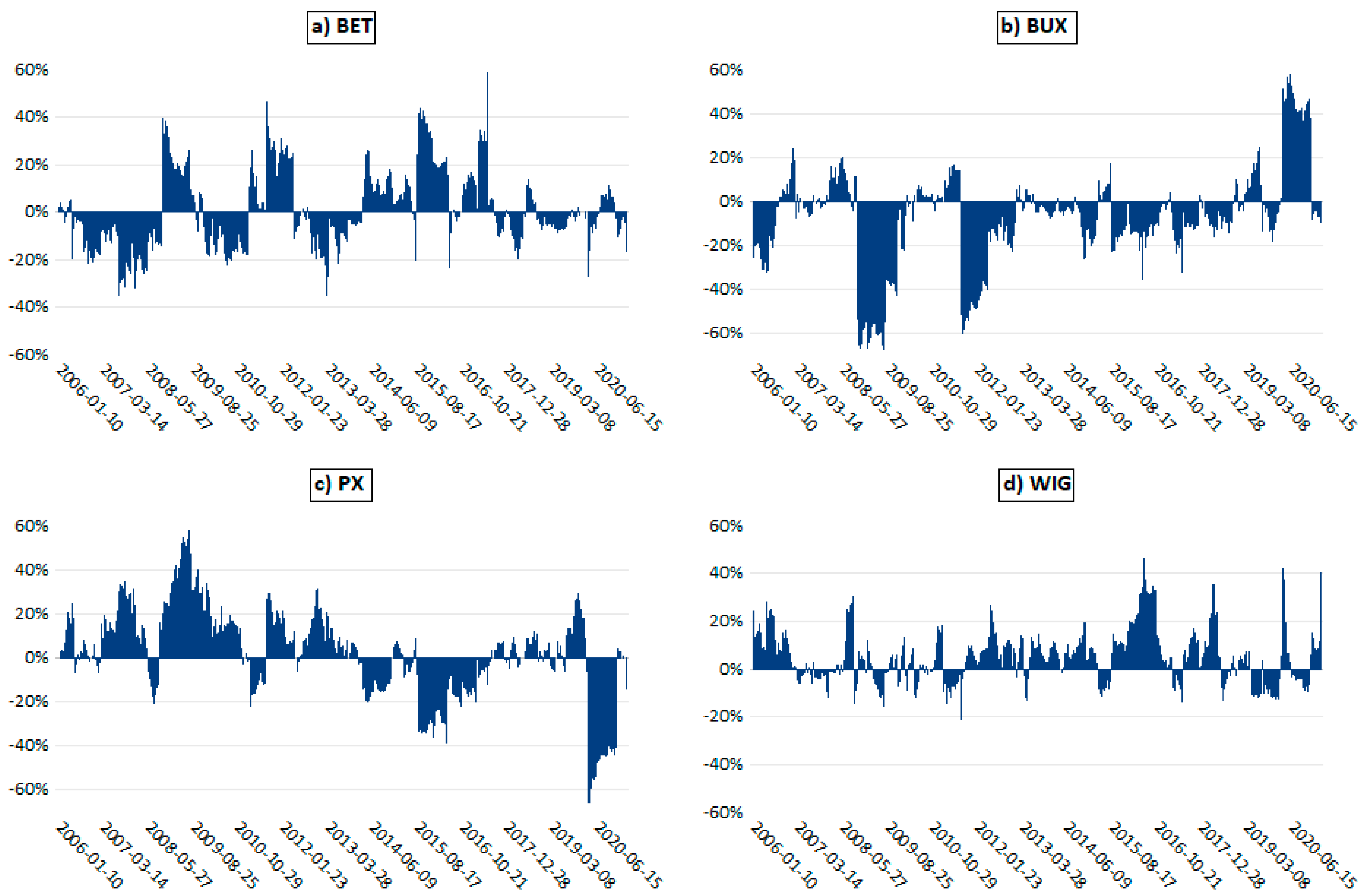
The effects of this economic crisis have also been felt strongly in the European financial markets. In Europe, the evolution of stock market indices at the end of 2008, compared to 2007, showed major decreases, with the German stock market index DAX falling by 40.4%. At the level of the four CEEC stock markets analyzed, the WIG index decreased by 48.2%, PX by 52.7%, and BUX by 53.3%. The BET index recorded the largest decrease, falling to 70% below the value at the end of 2007. It should also be noted that on 8 October 2008, because the volatility on the stock market was very high, it was necessary to suspend the Bucharest Stock Exchange’s trading activity for the day; this was the first time this had occurred in the exchange’s history.

By the end of 2009, large sovereign debts and significant budget deficits combined with high borrowing costs and the financial crisis, led to the collapse of the European Union’s financial system, also known as the European sovereign debt crisis. This began when Greece’s public debt reached 113% of its GDP in 2009, which was almost twice the 60% limit set in the euro area. Other countries, such as Ireland, Italy, Portugal, Cyprus, and Spain have followed in the footsteps of Greece, forming the GIIPS group. Each country requested financial assistance from the International Monetary Fund (IMF) and the EU to be able to emerge from the crisis.

The second DUMMY variable $D{M}_2$ takes the value 1 in the period 04 August 2011—28 November 2011 and 0 otherwise. The VIX index and the CISS index were used to choose this range, showing high volatility during this period. This interval is representative of the European sovereign debt crisis; at that time, there were concerns about the spread of the crisis to countries such as Spain and Italy. Stock market indices continued to experience severe volatility until the end of 2011. Moreover, stock indices in the United States, Europe, and Asia suffered significant declines in August 2011. This was because Standard & Poor’s downgraded the US credit rating for the first time in the agency’s history; it had been at AAA since 1941, but was reduced to AA+ on 6 August 2011.

To capture the recent crisis caused by the SARS-CoV-2 virus, two different DUMMY variables were used: $D{M}_3^{GE}$ and $D{M}_3^{SUA}$. DUMMY variable $D{M}_3^{GE}$, related to the correlation with the DAX index and takes the value 1 between 14 February 2020 (when the first death outside Asia was recorded, in France) and 27 December 2020 (when vaccination began in the European Union) and 0 otherwise. Variable $D{M}_3^{SUA}$, related to the correlation with the S&P500 index, takes the value 1 between 30 January 2020 and 27 July 2020 and 0 otherwise. This period was chosen given the remarkable volatility of the VIX index; on 30 January 2020, the COVID-19 outbreak was declared a Public Health Emergency of International Concern by the WHO.

The SARS-CoV-2 pandemic has affected the activity of international capital markets. This negative shock was triggered by the prospect of a new global crisis, by the fact that most economic activities have been frozen, and by the uncertainties about the evolution of the pandemic. In the first quarter of 2020, all stock market indices in the developed and the analyzed CEEC countries showed a negative trend (S&P500 −24.2%; DAX −28.7%; BET −25.7%; PX −31.4%; BUX −30%; WIG −30.5%). The BET index’s biggest decrease (−28.6% compared to the beginning of 2020) was recorded on 16 March 2020.

In March 2020, the Federation of European Securities Exchanges (FESE) recommended that the European stock markets continue to operate smoothly and respect regular operating hours despite the extreme market conditions caused by the COVID-19 pandemic. Stock exchanges were recommended to implement business continuity plans, thus remaining open for all investors to manage their portfolios in a transparent framework.

The estimation results of Equation (6) are given in Table 5. In the case of the correlation between the S&P500 index and the indices in the CEEC countries, all the coefficients of the DUMMY variables are positive and statistically significant (at the 5% level), for all of the three crises analyzed.

In the case of the correlation with the German stock market, the coefficients of the DUMMY variables $D{M}_1,D{M}_2$, $D{M}_3^{GE}$ are also positive and statistically significant (at the 5% level), except for the indices PX and BUX, for which $D{M}_1$ and $D{M}_2$ (only for BUX) are statistically insignificant. This analysis indicates a remarkable increase in the correlation between the stock indices analyzed during the previously identified crises, thus demonstrating the contagion phenomenon transmitted from the stock markets in Germany and the US to those in Central and Eastern Europe.

6. Capturing the Volatility Spillover Effect Using the Diebold-Yilmaz Methodology

6.1. Model Description

The computation of the volatility spillover index developed by [19] Diebold and Yilmaz (2012) starts from a variance decomposition matrix associated with a VAR model. The starting point represents the structural form of a VAR model with N variables, $x_t$= ($x_{1,t}$, …, $x_{N,t}$)′ (representing the volatilities), with t = 1, …, T, which takes into account p lags, as:

$$x_t={\displaystyle \sum }_{k=1}^p{\Phi }_k{x}_{t-k}+{\epsilon }_{t,}$$

(7)

where $\epsilon ~ \left(0,\mathsf{\Sigma }\right)$ is the vector containing independent and identically distributed errors, and ${\Phi }_k$, with k = 1, …, p, represents the coefficient matrices. In this model, each variable is put in regression with both its p lags and the p lags of the other variables in the system. In this way, the coefficient matrix contains complete information about the connections between variables.

The VAR process can be equivalently written as a vector moving-average (VMA): $x_t$ = ${\displaystyle \sum }_{k=0}^{\infty }{\mathrm{A}}_k{\epsilon }_{t-k}$. The n × n coefficient matrix ${\mathrm{A}}_k$ shall comply with the following expression: ${\mathrm{A}}_k={\mathsf{\Phi }}_1{\mathrm{A}}_{k-1}+\dots +{\mathsf{\Phi }}_p{\mathrm{A}}_{k-p}$, ${\mathrm{A}}_0$, being an identity matrix of size n × n and ${\mathrm{A}}_k=0$, for k < 0.

Starting from this specification, the impulse response functions and the forecast error variance decomposition will be used to analyze the interdependencies between variables. Variance decomposition is used to segment the forecast error variance for each variable into segments associated with different system shocks. An impulse response function tracks the effect of a shock occurring at some point in one of the model’s innovations on endogenous variables’ present and future values. If the innovations are simultaneously unrelated, the interpretation of the impulse response is relatively simple. Innovation i is simply a shock to variable i.

However, because innovations are usually correlated, to calculate the variance decomposition, orthogonal innovations based on identification schemes such as Cholesky factorization are necessary, but which scheme is used is dependent on the ordering of variables.

Therefore, to avoid this problem, Diebold and Yilmaz (2012) [19] used a generalized VAR framework proposed by Koop et al. (1996) [67,68] and Pesaran and Shin (1998), called KPPS. This framework constructs a set of non-orthogonal innovations that do not consider the order of variables within the VAR model. Instead of orthogonalizing shocks, the KPPS approach is based on generalized impulses. It allows correlated shocks but considers them using the historically observed distribution of the errors. Because the shocks are correlated, the sum of the contributions to the forecast error variance (the sum of the items on each row of the variance decomposition table) is not necessarily equal to 1.

In the volatility spillover index implemented by [19] Diebold and Yilmaz in 2012, the contribution of the variable $x_j$ to the forecast error variance of the variable $x_i$ (for i,j = 1,2,…,N, $i\ne j)$, at the time horizon h, is represented by:

$${\theta }_{ij}^g\left(H\right)=\frac{{\sigma }_{ii}^{-1}{{\displaystyle \sum }}_{\begin{array}{c}h=0\\ \end{array}}^{H-1}{\left(e_i^{\prime }{A}_h\Sigma e_j\right)}^2}{{{\displaystyle \sum }}_{h=0}^{H-1}\left(e_i^{\prime }{A}_h\Sigma A_h^{\prime }{e}_i\right)}$$

(8)

where $\mathsf{\Sigma }$ is the variance matrix for the error vector $\epsilon$, ${\sigma }_{ii}$ is the standard deviation of the error term for the $i^{th}$ equation, and $e_i$ is the selection vector with 1 as the $i^{th}$ element and 0 otherwise. As explained earlier, the sum of the elements on each row of the variance decomposition table is not necessarily equal to 1: ${\displaystyle \sum }_{j=1}^N{\theta }_{ij}^g\left(H\right)\ne 1$. To use the information available in the variance decomposition matrix to calculate the spillover index, each input of the variance decomposition matrix is normalized as follows:

$${\tilde{\theta }}_{ij}^g\left(H\right)=\frac{{\theta }_{ij}^g\left(H\right)}{{{\displaystyle \sum }}_{j=1}^N{\theta }_{ij}^g\left(H\right)}$$

(9)

In this way, ${{\displaystyle \sum }}_{j=1}^N{\tilde{\theta }}_{ij}^g\left(H\right)=1$ and $\left({{\displaystyle \sum }}_{i,j=1}^N{\tilde{\theta }}_{ij}^g\left(H\right)=N\right)$. Thus, the sum of all items ${\tilde{\theta }}_H$ (the sum of all the elements in the variance decomposition matrix) is equal to N.

6.1.1. Total Spillover Index

The model further constructs the total spillover index, which determines the contribution of the volatility spillover effect, combined from all variables to the total forecast error variance, as:

$$S^g\left(H\right)=\frac{{{\displaystyle \sum }}_{\begin{array}{c}i,j=1\\ i\ne j\end{array}}^N{\tilde{\theta }}_{ij}^g\left(H\right)}{{{\displaystyle \sum }}_{i,j=1}^N{\tilde{\theta }}_{ij}^g\left(H\right)}\ast 100=\frac{{{\displaystyle \sum }}_{\begin{array}{c}i,j=1\\ i\ne j\end{array}}^N{\tilde{\theta }}_{ij}^g\left(H\right)}{N}\ast 100$$

(10)

6.1.2. Directional Spillover

The generalized VAR approach allows the analysis of the directional spillover effect between asset classes. Because the generalized impulse responses and variance decomposition do not consider the order of variables, the directional spillover effect is calculated using the normalized elements of the variance decomposition matrix.

The directional spillover effect received by market i from all the other markets j is measured by the expression:

$$S_{i\leftarrow j}^g\left(H\right)=\frac{{{\displaystyle \sum }}_{\begin{array}{c}j=1\\ j\ne i\end{array}}^N{\tilde{\theta }}_{ij}^g\left(H\right)}{{{\displaystyle \sum }}_{j=1}^N{\tilde{\theta }}_{ij}^g\left(H\right)}\ast 100$$

(11)

Similarly, the directional spillover effect transmitted by market i to all the other markets j is measured by the expression:

$$S_{i\to j}^g\left(H\right)=\frac{{{\displaystyle \sum }}_{\begin{array}{c}j=1\\ j\ne i\end{array}}^N{\tilde{\theta }}_{ij}^g\left(H\right)}{{{\displaystyle \sum }}_{j=1}^N{\tilde{\theta }}_{ij}^g\left(H\right)}\ast 100$$

(12)

6.1.3. Net Spillover

The net volatility spillover from market i to all the other markets j is calculated as the difference between the gross volatility shocks transmitted to and the gross volatility shocks received from all other markets, as follows:

$$S_i^g\left(H\right)=S_{i\to j}^g\left(H\right)-S_{i\leftarrow j}^g\left(H\right)$$

(13)

6.1.4. Net Pairwise Spillover

The last type of volatility spillover, the net pairwise spillover between markets i and j, represents the difference between the gross volatility shocks transmitted from market i to market j and gross volatility shocks transmitted from j to i:

$$S_{ij}^g\left(H\right)=\left(\frac{{\tilde{\theta }}_{ij}^g\left(H\right)}{{{\displaystyle \sum }}_{k=1}^N{\tilde{\theta }}_{ij}^g\left(H\right)}-\frac{{\tilde{\theta }}_{ij}^g\left(H\right)}{{{\displaystyle \sum }}_{k=1}^N{\tilde{\theta }}_{ij}^g\left(H\right)}\right)\ast 100$$

(14)

6.2. Empirical Results and Discussions

To calculate the volatility spillover index developed by Diebold and Yilmaz (2012) [19], the conditional volatilities obtained from the GARCH (1,1) model (estimated in the first step of the DCC-GARCH model) were used. The index starts as a variance decomposition matrix associated with a VAR model, with the optimal lag 1 being chosen through the Schwarz Information Criterion (SIC). The analysis presented in Section 6.1 can be carried out statically over the whole period analyzed, but the chosen interval also contains subperiods of high volatility, such as those in the crises identified earlier. To capture the evolution of the volatility spillover index during turbulent periods, a dynamic version of the previous analysis is achieved through a rolling-window analysis, using a 200-day rolling sample window and a 10-day forecast horizon (h = 10), like that of [19] Diebold and Yilmaz (2012).

The elements on the ij positions ($i\ne j)$ in panel A of

Table 6. The volatility spillover effect in the CEEC stock markets—static.

Panel A. Directional Spillover Effect
Period April 2005–April 2021		From (j)				Contribution from Others
		BET	BUX	PX	WIG
To (i)	BET	0.715	0.062	0.139	0.084	0.285
	BUX	0.104	0.567	0.172	0.157	0.433
	PX	0.120	0.126	0.590	0.164	0.410
	WIG	0.078	0.135	0.160	0.627	0.373
Contribution to others		0.302	0.323	0.471	0.405	1.501
Total contribution		1.017	0.890	1.061	1.032	Total spillover index 0.375
Panel B. Net Pairwise Spillover.
		BET	BUX	PX	WIG	Conclusions
BET		0	−0.041	0.018	0.006	Net-transmitter
BUX		0.041	0	0.046	0.022	Net-recipient
PX		−0.018	−0.046	0	0.003	Net-transmitter
WIG		−0.006	−0.022	−0.003	0	Net-transmitter
Net volatility spillover		0.017	−0.109	0.061	0.031

correspond to the contribution of index $j$ to the forecast error variance of index $i$. In this way, the off-diagonal row sum shows the effect of directional volatility spillover received by each index from all the other indices (“Contribution from others”) and the off-diagonal column sum captures the effect of directional volatility spillover transmitted by each index to all the other indices (“Contribution to others”).

The value presented on the last line and the last column of panel A, the total spillover index, represents the percentage of the forecast error variance in all four stock markets that is due to the volatility spillover phenomenon. This is calculated as the off-diagonal sum of all elements on the rows, divided by the sum of all elements in the matrix (or the number of variables analyzed, N = 4).

Panel B from Table 6 presents the net pairwise spillover, which is calculated as the difference between the gross shocks of volatility transmitted from index i to index j and the gross volatility shocks transmitted from j to i (situated in panel A).

The sum of the items on the columns represents the net volatility spillover, shown in the last row of panel B, from index i to all the other indices. The net volatility spillover can also be calculated as the difference between the (‘Contribution to Others’ and ‘Contribution from Others’). If this indicator is positive, that index transmits net volatility (“Net-transmitter”), and if the value is negative, the index receives net volatility (“Net-receiver”).

Table 6 indicates that, on average, between 1 April 2005 and 1 April 2021, 37.5% of the forecast error variance in these emerging stock markets comes from the spillover phenomenon. All the elements on the main diagonal have much higher values than the others, which suggests that own market volatility spillovers (own shock contributions) explain the highest share of forecast error variance.

As Table 6 shows, the stock markets in Poland, the Czech Republic, Romania, and Hungary, the largest CEEC countries, are well integrated. All the stock markets analyzed are affected by the volatility of the other markets, which indicates bidirectional volatility spillovers rather than unidirectional volatility spillovers. However, it is noted that the stock markets in Poland, the Czech Republic, and Hungary are more integrated compared to the Romanian stock market. These three countries joined the European Union at the same time (1 May 2004) and are part of an economic and political cooperation group called the Visegrad Group (1991), together with Slovakia. Even before entering the EU, the four countries had a free trade convention between these four countries that led to increased economic cooperation between them.

In Table 6, the values for the directional spillover effect received by each index from all the other indices (the ‘Contribution from Others’ section) vary between 28.5% and 43.3%. These are calculated as the difference between 100% and its contribution to the forecast error variance (the value on the diagonal of panel A) for each stock market index. The BUX and PX indices receive the highest volatility from the remaining stock indices analyzed (43.3% and 41.0%, respectively), while the lowest amount of volatility received is recorded for the BET index (28.5%).

Similarly, the values for the directional spillover effect transmitted by each index to all the other indices (“Contribution to Others”) vary between 30.2% and 47.1%. The Czech and Polish stock market index transmits the highest volatility to the rest of the indices, namely 47.1% (PX) and 40.5% (WIG).

The last row of panel B reflects the net contribution of each stock market index. The positive value means that the stock index transmits net volatility, and the negative value means that it receives net volatility. Of the four indices analyzed, three are net volatility transmitters, with the highest value being recorded by the PX index (6.1%), and the only net volatility recipient is the BUX index, with a value of (−10.9%).

It is noted that the BET index transmits and receives the lowest volatility compared to the rest of the indices. The basket of the Bucharest Stock Exchange’s reference index, BET, currently includes the shares of the 17 blue-chip companies, meaning that it tracks the performance of the most traded and liquid companies on the Bucharest Stock Exchange. At the beginning of June 2021, the shares of Banca Transilvania, Fondul Proprietatea, and OMV PETROM held over 50% (the largest share) in the basket of the BET index. Of the 17 companies, 15 are Romanian and 2 are foreign, i.e., PURCARI Wineries (Cyprus) and Digi Communications N.V. (Amsterdam, the Netherlands); these two companies hold 4.17% of the BET index.

According to Table 6, the PX index transmits the highest volatility to the other indices of the CEEC countries analyzed and is also a net transmitter, recording the highest value of net volatility spillover (6.1%). It is worth mentioning the particularity of the Prague Stock Exchange, which is captured in Appendix A: during the entire period under review, it has the highest share of foreign companies in total listed companies, reaching over 60% after 2018. Currently, the basket of the PX index consists of 13 companies; 7 are Czech, and 6 are foreign, and the share of foreign ones has increased to 50.16%. Erste GROUP BANK (Austria) holds the highest share in the PX index (21.81%). The largest shareholder of the Prague Stock Exchange (PSE) since December 2008 is Wiener Börse AG (Vienna Stock Exchange), which currently holds 99.54% of the shares.

Table 6, although it provides a valuable summary of the average spillover effect during the chosen time frame, is a static analysis and cannot capture the evolution of this effect during periods of crisis that have had a major impact on stock markets around the world, including the CEEC stock markets analyzed. Therefore, to analyze the volatility spillover effect during turbulent periods, a rolling window estimation was created that used a 200-day rolling sample and a time horizon of 10 days (“ten-day forecast horizon”). The results are shown in Figure 5.

As can be seen, the total spillover index varies greatly over the considered interval, between 6% (at the end of 2013, after the European sovereign debt crisis) and 67% (in March 2020, when COVID-19 was officially declared a global pandemic by the WHO). In general, during turbulent periods such as the Great Recession, the European sovereign debt crisis, and the crisis caused by the SARS-CoV-2 virus, this index increased significantly, registering values of over 60% (over 60% of the forecast error variance of all analyzed CEEC stock markets comes from the spillover phenomenon). The results have been confirmed by the findings of [64,69] Papathanasiou et al.(2022a, b), [70] Balcilar et al.(2021), [71] Yousaf and Yarovaya(2022) and [42] Samitas et al.(2022), showing that spillover effects tend to increase during turbulent periods, such as European Sovereign Crisis and COVID-19 pandemic. According to Papathanasiou et al.(2022a) [64], dynamic connectedness showed accretion during periods of turmoil, such as the US–China trade war, COVID-19, and the Russia–Ukraine war, indicating that volatility spillovers are prone to extraneous shocks. Similar results have also been proven by the findings of Papathanasiou et al. (2022b) regarding moderate volatility spillovers, which increased during the highlighted turbulent periods.

Balcilar et al.(2021) [70] analyzed the interconnectedness of crude oil and agricultural commodity assets, revealing that the connectedness is heterogeneous over time and driven by economic events reaching peaks during the GFC, European governmental debt crisis, and the recent COVID-19 pandemic. Yousaf and Yarovaya (2022) [71] and Samitas et al. (2022) [42] also confirmed that the volatility connectedness increased during the initial phase of the COVID-19 pandemic.

Similarly, Figure 5 presents the effects of net volatility spillover for each stock market index using a rolling-window analysis. This is calculated as the difference between the directional spillover transmitted by each index to all other indices (Appendix K) and that received by each index from all other indices (Appendix L). As mentioned above, a bidirectional volatility spillover phenomenon can be observed once again. All stock market indices analyzed show periods during which they transmit net volatility (‘net transmitter’—periods during which positive values are recorded) and periods during which they receive net volatility (‘net recipient’—periods during which negative values are recorded).

The BET, WIG, and PX indices were net transmitters of volatility for most of the period analyzed. During the Great Recession and the European sovereign debt crisis, the PX index and the BET index both transmitted net volatility, which was particularly received by the BUX index.

Although the Polish stock market, WIG, is a net transmitter for almost the entire period examined, the magnitude of the net volatility transmitted is much lower than that given by the above-mentioned BET and PX indices. The only exception is the period 2015–2016, when the net volatility transmitted by the WIG index was over 40%. Beginning in 2014, in addition to the turbulent international events mentioned above, Poland felt the strong effects of private pension fund reform. Through this reform, 51.5% of these funds were transferred to a state institution. Previously, private pension funds invested these funds in local shares listed on the Warsaw Stock Exchange. In 2016, Poland also experienced numerous protests regarding the new conservative government and the measures it took which affected the power of the Constitutional Court and the freedom of the press, and a potential total ban on abortions.

As for the BUX index, it was a net volatility recipient for most of the period analyzed, except for one point during the COVID-19 crisis. Between April and December 2020, the reference index of the Hungarian stock market, BUX, transmitted net volatility of over 50% to the other three stock indices in the CEEC. This aspect is analyzed in detail in Figure 6, where the net pairwise spillover effects are presented.

A rolling window estimation, similar to the previous ones, was also used to achieve a net pairwise spillover index, and the results are shown in Figure 6. This indicator is calculated as the difference between the volatility transmitted from index i to index j and the volatility transmitted from index j to index i.

From the analysis of the relationships between all 6 pairs of stock indexes presented in Figure 7, it is noted that none of the four indices have a dominant position as a net transmitter for the whole period under observation.

Regarding the relationship between BET and PX indices, in the first part of the period analyzed, BET receives net volatility from PX; this relationship is reversed after 2013. A similar situation is found in between the Polish index, WIG, and the Czech index, PX.

As mentioned above, during the crisis caused by the SARS-CoV-2 virus, the BUX index transmitted net volatility to all the other stock indexes analyzed from the CEEC. In the first part of 2020, the outbreak of the COVID-19 pandemic created high volatility on the stock markets. The October 2020 Global Financial Stability Report (biannual publication of the International Monetary Fund) also included the impact of the SARS-CoV-2 crisis on global capital markets. This report mentioned that capital markets which were dominated by sectors such as information technology and telecommunications were least affected by the pandemic. Markets that are dominated by the financial and the energy sectors (energy, oil, natural gas) have seen major declines in stock market performance. The crisis caused by the COVID-19 pandemic has deteriorated the quality of assets in banks’ balance sheets and accentuated the risk of accumulation of non-performing loans.

Analyzing the sector breakdown of the four CEEC stock indices, it follows that in the case of BUX, BET and PX, more than 60% of the market capitalization is the banking and energy sectors, as opposed to the Polish index, WIG, where the share was only 20%.

Moreover, in the basket of the BUX index, which transmitted net the highest volatility during the COVID-19 crisis, a very high percentage (40.70%) is owned by a single company from the banking sector—OTP Bank. In the first semester of last year, this company recorded a decrease in the consolidated net profit of 58% compared to the same period of the previous year (according to the Financial Report for the first semester of 2020 published by OTP BANK Plc.). Therefore, this was also reflected in the magnitude of volatility spillovers during this period, with the volatility transmitted by the BUX index to the BET and the PX being around 22% and 30%, respectively.

The 2020 Romanian Financial Stability Report, issued by the Financial Supervisory Authority (FSA), stated that the volatility of the Romanian stock market had evolved on a trend similar to that of foreign markets and the financial and energy sectors, which are predominant in the capitalization of the local stock exchange. These sectors also experienced the most volatile developments during this period at the international level.

7. Exploring the Contagion EFFECT during the COVID-19 Pandemic Using Markov Switching Regime VAR Approach

Furthermore, we investigated the contagion effect between developed stock markets and CEE markets, exploring the regime swift across sanitary crisis using a Markov regime-switching VAR framework. The impacts of shocks are not anticipated to remain constant throughout time and may occasionally undergo regime modifications.

7.1. Methodology and Data

We used a multivariate Markov switching vector autoregressive (MS-VAR) framework within our analysis with two regimes that allow the mean and variance to change concurrently, following [72] Krolzig (1997). The period used was 1 January 2018–4 April 2021.

The main element of innovation of the MS-VAR approach is that the dynamic structures depend on the value of the state variable, $s_t$, which controls the switching mechanism between various states.

$$Y_t=v{\left(s\right)}_t+A_1\left(s_t\right)·Y_{t-1}+\dots A_p\left(s_t\right)·Y_{t-p}+{\epsilon }_t$$

(15)

where $Y_t$ is a six-dimensional time series vector that includes the returns of all four CEE stock markets combined with the returns of S&P 500 and DAX; v is a 6 × 6 matrix of intercepts, $A_{1,\dots }{A}_p$ are matrices containing the autoregressive parameters and ${\epsilon }_t$ is a white noise vector. $s_t$ is a random variable defined:

$$\sum S\left(t\right)=(\begin{array}{cc}{\sigma }_{1, s\left(t\right)}^2& {\sigma }_{12,s\left(t\right)}\\ {\sigma }_{21, s\left(t\right)}& {\sigma }_{2,s\left(t\right)}^2\end{array})$$

(16)

In a first-order Markov process, the current regime $s_t$ depends on the regime one period ago, $s_{t-1}$:

$P\left(s_t=j|s_{t-1}=i, s_{t-2}=k,\dots .\right)=P\left(s_t=j|s_{t-1}=i\right)=p_{ij}$, pij is the transition probability from one regime to another. Fom m regimes, the transition probabilities are formalized into a (mxm) transition matrix (P), as follows:

$$P=\left(\begin{array}{ccc}{p}_{11}& \cdots & p_{1m}\\ ⋮& \ddots & ⋮\\ p_{m1}& \cdots & p_{mm}\end{array}\right)$$

(17)

with ${\displaystyle \sum }_{j=1}^m{p}_{ij}=1$ where $i=1,2\dots ..m$ and $0\le p_{ij}\le 1$.

The transition probabilities also provide the expected duration for regime j(Dij):

$$E{\left(D\right)}_{ij}=\frac{1}{1-p_{ij}}, j=1, 2\dots ..m$$

(18)

Within the study, we assumed two states ($s_1$ and $s_2$) representing two regimes: one with high volatility and another with low volatility. The higher the values of $p_{11}$ and $p_{22}$, the more likely the hypothesis of no regime shift would be rejected.

It would be more enlightening if we looked further into the various market performances in the “risky” regime (corresponding to greater means and higher volatilities) as well as in the “stable” regime (associated with smaller means and lower volatilities).

In the next step, we conduct impulse response function analysis to quantify and trace the time paths of the effects of developed stock markets on the CEE markets. One advantage of applying the generalized impulse response function (GIRF) is that it is invariant with the order of the variables in the VAR system.

7.2. Empirical Results

In the first stage, the order of integration of each variable has been identified using unit-root tests (ADF and PP tests) as well as the optimal lag length (k) of the VAR system based on Schwarz Bayesian (SBC) as begin 1. The absence of residual serial correlation of the individual equations has also confirmed the correct order of VAR selection. The residual series passes the required diagnostic tests for serial correlation and heteroscedasticity. Therefore, we explore the relationships of [RSP, RDAX, RBET, RBUX, RPX, RWIG] within a Markov regime-switching VAR framework, which allows the influence of explanatory variables to be state-dependent.

The empirical results of MS-VAR are displayed in

Table 7. Markov regime-switching VAR results.

	RSP	RDAX	RBET	RBUX	RPX	RWIG
	Regime 1
RSP(-1)	−0.1689	−0.0479	−0.2081 **	−0.2131 **	−0.3977 ***	0.3468 ***
RDAX(-1)	1.3604 ***	−0.6008	1.7477 ***	−0.9532 ***	−0.2608	−0.1700
RBET(-1)	−0.0734	0.0581	−0.8968 ***	−0.0164	−0.2198	0.2033
RBUX(-1)	−0.8398	−0.5360	−0.9094 ***	−0.7173 ***	−0.6535 ***	−0.4479 ***
RPX(-1)	0.0403	1.7317	−0.2375	1.8071 ***	1.4049 ***	0.6548 **
RWIG(-1)	−1.289382	−0.166283	−0.222990	0.180256	0.217065	−0.503581 **
	Regime 2
RSP(-1)	−0.1493 ***	0.2641 ***	0.0758	0.2385 ***	0.2015 ***	0.1485 ***
RDAX(-1)	−0.0256	−0.2136 ***	0.0017	−0.1656 **	−0.0684	−0.1156*
RBET(-1)	0.0654	0.0409	0.0363	0.0207	0.0920 **	0.0316
RBUX(-1)	−0.0743	−0.0513	0.0177	−0.0296	−0.0241	−0.0347
RPX(-1)	0.1471	0.1063	−0.0615	0.2175**	−0.0267	−0.0284
RWIG(-1)	0.0577	0.0387	0.0605	0.0939	0.0349	0.1421 *

Note: *, **, *** implies significant at 10%, 5% and 1% level of significance.

. In regime 1, the shock in the US stock market significantly impacted stock markets in Hungary, Poland, and the Czech Republic. The German stock market significantly impacted the Romanian and Hungarian stock markets. The stock market from Hungary also had a significant impact on the Polish, Romanian, and Czech Republic stock markets.

In regime 2, the US stock market statistically impacted all four CEE and the German stock markets, while the German stock market significantly affected the Hungarian and Polish stock markets. There is also a link between the Czech and Hungarian stock markets. The transition probability matrix reveals that regime 2 is highly persistent. Therefore, regime 2 will persist for 59 days (

Table 8. Transition probability matrix.

	1	2
1	0.273	0.7262
2	0.0168	0.9831

and

Table 9. Expected duration of each regime.

1	2
1.3769	59.248

).

The smoothed regime probabilities depicted in Figure 8 reveal that the watershed of two regimes for the markets occurred on 18 March 2020.

The effects of a shock in the developed stock markets on the CEE stock markets have been evaluated using the GIRF tracking the impulse response to the shock for an horizon of 10 days. The results are displayed in Appendix M and Appendix N.

Appendix M displayed the effects of CEE stock markets to a shock in the US stock market in both regimes. The strongest response of S&P 500 1-day innovation is evaluated on the German stock market in both regimes, followed by the Polish stock market, while on the opposite side, there is the Czech stock market. Analyzing the effects of the shock at a 2-day horizon, the Hungarian and Czech stock markets revealed the highest decline in the first regime, while Poland is the only one that exhibited a positive effect.

In the second regime, all markets pointed out positive impacts, with the strongest effects registered by Hungarian and Czech stock markets. A shock of one standard deviation of the US stock market implies an approximately 0.58% decline in the Hungarian stock market in the first regime and a 0.30% increase in the second regime. A 1% increase in the S&P 500 revealed a 0.19% response in the German stock market in the second regime.

Analyzing the effects of a German stock market on the CEE stock markets in both regimes (Appendix N), it can be highlighted that the Czech and Hungarian stock markets register the strongest response for 1-day horizon. Analyzing the effects of the shock at the horizon of a 2-day, in the first regime, the Hungarian and Czech stock markets revealed the highest decline, while in the second regime, all markets pointed out positive impacts, the strongest effects being registered by Hungarian and Czech stock markets.

A one-standard-deviation shock of the German stock market implies approximately a 0.70% decline in the Hungarian stock market in the first regime and a 0.19% increase in the second regime.

Furthermore, the variance decomposition analysis provides additional valuable about the relative strengths of various shocks to the innovations of the variables in the economic system (Appendix O). The shock from the US and German stock markets had the strongest impact on Polish and Czech stock markets, irrespective of the regime.

Analyzing the response of the Romanian stock market to the system shocks, it should be highlighted that, apart from its innovations, the stock market in the first regime was mostly interconnected with the Hungarian stock market and only marginally with the US and German stock markets, which accounts for nearly 7.27% and 5.85% of the BET index, respectively, at the horizon of the 10th day. In the second regime, the US stock market accounted for 21.61% of the variation of the BET index, while the German stock market accounted for 5.99%.

In the first regime, the Hungarian stock market was interconnected with the Romanian stock market, which explains almost 27.21% of the variation, followed by the US and German stock markets with 8.39% and 7.38%. In the second regime, US stock market accounts for almost 26.82% of the BUX index, while the German stock market nearly 12.96%.

The Polish stock market was strongly interconnected in the first regime with The Hungarian and Romanian stock markets, which accounted for almost 50.14% of the total variation, respectively 27.48% at the 10-day horizon, the developed stock markets having only a marginal contribution. However, in the second regime, the US stock market explained nearly 32.20% of the total variation, while the German stock market almost 17.6%.

In the case of the Czech stock market, the first regime was governed by connections with Hungarian and Romanian stock markets, the US and German stock markets explaining around 10% of the total variation. In the second regime, the US stock market explained 29.42% of the total variation, while the German market 17% of PX index.

Analyzing the contagion channel through the impulses of US stock market to CEE stock markets, its explanatory power increases from 10.38% in regime 1 in the case of the Czech stock market, to almost 32.20% of the total variation in regime 2 in the case of Polish stock market. In the case of the German stock market, the increase was smaller between both regimes, from 7.49% in regime 1 to 17.63% in regime 2. The empirical evidence revealed clearly that these markets were highly correlated during the pandemic crisis period.

8. Summary and Conclusions

This paper analyzed the existence of the contagion effect from developed stock markets (Germany and US) to the emerging ones in Central and Eastern Europe (Romania, Czech Republic, Hungary, and Poland) from the perspective of the reference stock market indices in the period 2005–2021.

The contagion effect was captured by estimating conditional correlations based on the DCC-GARCH model. The analysis of these dynamic correlation coefficients has demonstrated the propagation of shocks from the stock markets in the developed countries to those in the emerging countries of Central and Eastern Europe. Grabowski (2019) [11] also proved the existence of high correlations between shocks produced in the CEE-3 nations during unstable times, which suggests that the Visegrad countries engaged in herding tendencies throughout the financial instability, the US subprime crisis, and the euro area sovereign debt crisis.

Throughout the period under analysis, the Polish stock market has proved to be the most correlated with the two developed markets since it is the largest in the Central and Eastern European area and the only one classified by FTSE Russell in the Developed Market category. By contrast, the Romanian stock market is the least correlated with that in the US and Germany, as it is the last market in this region classified as emerging by FTSE Russell. Grabowski (2019) [11] and Bein and Tuna (2015) [52] also acknowledged the higher conditional correlation of the Polish and Czech stock markets with Germany and the US compared to Hungary.

During the Great Recession, the European sovereign debt crisis, and the SARS-CoV-2 pandemic, correlation coefficients from the DCC-GARCH model saw significant increases, indicating propagation of shocks from developed markets to emerging ones. This result is also confirmed by the literature through the studies of [6] Chiang et al. (2007), [29] Li and Majerowska (2008), and [8] Syllignakis and Kouretas (2011).

The quantification of the contagion effect during times of crisis was also carried out through an analysis based on 3 DUMMY variables, specific to each of the crises identified above. In selecting the crisis periods, the VIX volatility index and the Composite Indicator of Systemic Stress (CISS) were also used, and their evolution capturing stock markets’ the turbulent periods well.

Moreover, by using a rolling stepwise regression (Appendix I and Appendix G), it has been noted that the conditional correlations between the DAX index and four CEEC stock indices increase with the volatility on the German stock market, especially during periods of crisis. This result limits the benefit of portfolio diversification for investors who choose to trade on both the German stock market and the analyzed CEEC stock markets, especially in times of crisis.

The volatility spillover index implemented by [19] Diebold and Yilmaz in 2012 surprised the high level of integration of the analyzed stock markets in Central and Eastern Europe, with the intensity of volatility transmission between these markets increasing significantly during times of crisis. It is worth mentioning that the reference index of the Romanian stock market transmits and receives the lowest volatility compared to the rest of the CEEC stock indices analyzed, which indicates that Romania is less integrated with Poland, the Czech Republic, and Hungary.

The total volatility spillover index recorded an average value of 37.5% between 2005 and 2021, meaning that 37.5% of the forecast error variance in all of the CEEC stock markets comes from the spillover phenomenon. During the COVID-19 pandemic, this index recorded the highest value over the entire time horizon (over 60%).

All stock market indices analyzed show periods during which they transmit net volatility and periods during which they receive net volatility, indicating a bidirectional volatility spillover phenomenon. For the most part, the BET, PX, and WIG indices are net transmitters of volatilities, whereas the BUX index is a net recipient, except during the COVID-19 crisis, when it transmitted net volatility to all the other 3 indices.

According to Grabowski (2019) [11], the stock markets of Poland, the Czech Republic, and Hungary are volatility takers, receiving volatility from the American and German stock markets.

During COVID-19 pandemic, the stock markets that were dominated by the financial and energy sectors were most affected. This included the reference indices of the stock markets in Romania (BET), the Czech Republic (PX), and Hungary (BUX), which have more than 60% of the market capitalization in these two sectors. However, a very high percentage (40.70%) of the basket of the BUX index is owned by a single company in the banking sector, which recorded major losses in the first semester of last year (2021).

Furthermore, using a Markov switching regime VAR approach, the contagion effect from developed stock markets to emerging CEE markets has been captured covering the most recent sanitary crisis when markets exhibited regime shifts. The empirical results proved the shift that occurred around the beginning of the health crisis, after which the high volatility regime dominated the CEE markets. The impulse response functions pointed out that the contagion effects from developed stock markets to emerging CEE markets are more persistent during the sanitary crisis. The variance decomposition analysis revealed that the shock from the US and German stock markets had the strongest impact on Polish and Czech stock markets, irrespective of the regime. However, the empirical evidence revealed clearly that these markets were highly correlated during the pandemic crisis period.

By being aware of the key variables that affect the spillover effects of the CEE stock markets, policymakers may decide on the best course of action to lessen the spread of shocks. Our study’s conclusions provide crucial data for developing policies that would minimize the susceptibility of CEE markets to shocks from developed economies.

Our findings showed that CEE stock markets were interdependent with respect to those of the US and Germany, and that this interdependence was particularly pronounced during systemic events like the 2007–2008 global financial crisis, the 2008 European governmental debt crisis, and the most recent COVID-19 pandemic. These insights are of the highest importance to risk and portfolio managers who are developing their investing and hedging strategies to satisfy their risk-return objectives. Here, we show how the whole network is impacted by a shock to one stock market. If a portfolio manager had a portfolio that contained all of those assets, they would be well aware of the risk spillovers since the findings of our study may be used as an early warning signal for possible spillovers. This study illustrates how much the shock will impact other markets as a result. Overall, our findings support [73] Asongu (2012) and [74] Bekaert (2014) which state that financial contagion from the US stock market to the CEE markets occurs regardless of the financial crisis period, but we find that contagion is stronger during the crisis (sensitivity to unexpected negative events increases considerably). As noted by several studies [40,42,64,66,67,69,75,76], the stock index is the main net transmitter that suggests the utility of considering spillovers of higher moments and jumps when studying the CEE stock market in concordance with US or German stock markets.

The first implication of this study is that there always exists some degree of contagion. First, in order to create appropriate frameworks to prevent financial instability, policymakers, governments, and regulators should understand the dynamic interconnections among the markets that are seen, particularly during crisis situations where connectivity tends to accelerate, such as during the pandemic. The second implication is significant for global investors because they suggest that diversity sought by investing in a number of markets from various geographical blocks is likely to be less effective when it is most desired. As a result, an investing strategy that only emphasizes foreign diversity appears to fail in reality during times of financial unrest with a highlight on COVID-19 pandemics. From the standpoint of decision makers, this study offers crucial knowledge about the different routes for adopting actions to safeguard developing markets from spreading crises. Decision makers should carefully consider and identify any potential decoupling tactics that could protect developing markets from spreading instability. Specifically, markets will have a high inclination to respond negatively to events that would not normally deserve a significant reaction when a fall in investors’ appetite for risk occurs following a time of high appetite for risk.

From the policy makers’ perspective, since the emerging CEE markets are very sensitive to high volatility from developed stock markets, the level of uncertainty in those markets needs to be monitored, especially the negative shocks among CEE countries.

As the main limitations of the study, we can point out the limited number of CEE countries, and a potential extension of the research would include Estonia (TALSE), Slovakia (SAX12), and Slovenia (SBI). The relatively small period of sanitary crisis that was also captured in our analysis offers a possibility to extend the analysis in the near future by including additional observations within the sample. Another opportunity would be to extend the analysis by including Russia since it was the largest stock market in the CEE region in terms of market capitalization, and since Russia remains the dominant regional economic and political power, with significant trade links with the rest of the CEE countries as well as a significant source of direct investment in the region.

Given the results of the study, future research directions of interest may include the extension of the analysis of the contagion effect to a greater number of emerging stock markets in Central and Eastern Europe and the inclusion of more developed markets as influence factors.

Another research direction to further explain the volatility spillover effect on financial markets could be an analysis of the monetary and fiscal policy shocks on stock markets. This could extract the effect of these policies’ shocks based on the volatility of the shock indices.

References

1. Lessard, D.R. World, national, and industry factors in equity returns. J. Financ. 1974, 29, 379–391. [Google Scholar] [CrossRef]
2. Solnik, B.H. Note on the validity of the random walk for European stock prices. J. Financ. 1973, 28, 1151–1159. [Google Scholar] [CrossRef]
3. Dornbusch, R.; Park, Y.C.; Claessens, S. Contagion: Understanding how it spreads. World Bank Res. Obs. 2000, 15, 177–197. [Google Scholar] [CrossRef] [Green Version]
4. Forbes, K.J.; Rigobon, R. No contagion, only interdependence: Measuring stock market comovements. J. Financ. 2002, 57, 2223–2261. [Google Scholar] [CrossRef]
5. Yang, S.Y. A DCC analysis of international stock market correlations: The role of Japan on the Asian Four Tigers. Appl. Financ. Econ. Lett. 2005, 1, 89–93. [Google Scholar] [CrossRef]
6. Chiang, T.C.; Jeon, B.N.; Li, H. Dynamic correlation analysis of financial contagion: Evidence from Asian markets. J. Int. Money Financ. 2007, 26, 1206–1228. [Google Scholar] [CrossRef]
7. Phylaktis, K.; Ravazzolo, F. Stock market linkages in emerging markets: Implications for international portfolio diversification. J. Int. Financ. Mark. Inst. Money 2005, 15, 91–106. [Google Scholar] [CrossRef]
8. Syllignakis, M.N.; Kouretas, G.P. Dynamic correlation analysis of financial contagion: Evidence from the Central and Eastern European markets. Int. Rev. Econ. Financ. 2011, 20, 717–732. [Google Scholar] [CrossRef]
9. Grabowski, W.; Rotuski, K.; Skrzypczak, K. An Analysis of Technical Factor Returns on the Warsaw Stock Exchange, 1999–2009; Ekonomia/Uniwersytet Warszawski: Warszawa, Poland, 2011; pp. 166–172. [Google Scholar]
10. Horvath, R.; Lyócsa, Š.; Baumöhl, E. Stock market contagion in Central and Eastern Europe: Unexpected volatility and extreme co-exceedance. Eur. J. Financ. 2018, 24, 391–412. [Google Scholar] [CrossRef] [Green Version]
11. Grabowski, W. Givers or recipients? Co-movements between Stock Markets of CEE-3 and developed countries. Sustainability 2019, 11, 6495. [Google Scholar] [CrossRef]
12. Bae, K.H.; Karolyi, G.A.; Stulz, R.M. A new approach to measuring financial contagion. Rev. Financ. Stud. 2003, 16, 717–763. [Google Scholar] [CrossRef]
13. Samarakoon, L.P. Stock market interdependence, contagion, and the US financial crisis: The case of emerging and frontier markets. J. Int. Financ. Mark. Inst. Money 2011, 21, 724–742. [Google Scholar] [CrossRef]
14. Siddiqui, T.A.; Khan, M.F.; Naushad, M.; Syed, A.M. Cross-Market Correlations and Financial Contagion from Developed to Emerging Economies: A Case of COVID-19 Pandemic. Economies 2022, 10, 147. [Google Scholar] [CrossRef]
15. Goodell, J.W. COVID-19 and finance: Agendas for future research. Financ Res Lett. 2020, 35, 101512. [Google Scholar] [CrossRef] [PubMed]
16. So, M.K.; Chu, A.M.; Chan, T.W. Impacts of the COVID-19 pandemic on financial market connectedness. Financ. Res. Lett. 2021, 38, 101864. [Google Scholar] [CrossRef]
17. Albulescu, C.T. COVID-19 and the United States financial markets’ volatility. Financ Res Lett. 2021, 38, 15309. [Google Scholar] [CrossRef] [PubMed]
18. Nguyen, T.N.; Phan TK, H.; Nguyen, T.L. Financial contagion during global financial crisis and covid–19 pandemic: The evidence from DCC–GARCH model. Cogent Econ. Financ. 2022, 10, 2051824. [Google Scholar] [CrossRef]
19. Diebold, F.X.; Yilmaz, K. Better to give than to receive: Predictive directional measurement of volatility. Int. J. Forecast. 2012, 28, 57–66. [Google Scholar] [CrossRef] [Green Version]
20. King, M.; Sentana, E.; Wadhwani, S. Volatile and Links between National Stock Markets (No. w3357); National Bureau of Economic Research: Cambridge, MA, USA, 1990. [Google Scholar]
21. Lee, S.B.; Kim, K.J. Does the October 1987 crash strengthen the co-movements among national stock markets? Rev. Financ. Econ. 1993, 3, 89–102. [Google Scholar] [CrossRef]
22. Akhtaruzzaman, M.; Boubaker, S.; Sensoy, A. Financial contagion during COVID-19 crisis. Financ. Res. Lett. 2021, 38, 101604. [Google Scholar] [CrossRef]
23. Dimitriou, D.; Kenourgios, D.; Simos, T. Global financial crisis and emerging stock market contagion: A multivariate FIAPARCH–DCC approach. Int. Rev. Financ. Anal. 2013, 30, 46–56. [Google Scholar] [CrossRef]
24. Hwang, E.; Min, H.G.; Kim, B.H.; Kim, H. Determinants of stock market comovements among US and emerging economies during the US financial crisis. Econ. Model. 2013, 35, 338–348. [Google Scholar] [CrossRef]
25. Min, H.G.; Hwang, Y.S. Dynamic correlation analysis of US financial crisis and contagion: Evidence from four OECD countries. Appl. Financ. Econ. 2012, 22, 2063–2074. [Google Scholar] [CrossRef]
26. Yousfi, M.; Zaied, Y.B.; Cheikh, N.B.; Lahouel, B.B.; Bouzgarrou, H. Effects of the COVID-19 pandemic on the US stock market and uncertainty: A comparative assessment between the first and second waves. Technol. Forecast. Soc. Change 2021, 167, 120710. [Google Scholar] [CrossRef] [PubMed]
27. Luchtenberg, K.F.; Vu, Q.V. The 2008 financial crisis: Stock market contagion and its determinants. Res. Int. Bus. Financ. 2015, 33, 178–203. [Google Scholar] [CrossRef]
28. Cappiello, L.; Engle, R.F.; Sheppard, K. Asymmetric dynamics in the correlations of global equity and bond returns. J. Financ. Econom. 2006, 4, 537–572. [Google Scholar] [CrossRef]
29. Li, H.; Majerowska, E. Testing stock market links for Poland and Hungary: A multivariate GARCH approach. Res. Int. Bus. Financ. 2008, 22, 247–266. [Google Scholar] [CrossRef]
30. Caporale, G.M.; Spagnolo, N. Stock market integration between three CEECs, Russia, and the UK. Rev. Int. Econ. 2011, 19, 158–169. [Google Scholar] [CrossRef] [Green Version]
31. Kenourgios, D.; Samitas, A.; Paltalidis, N. Financial crises and stock market contagion in a multivariate time-varying asymmetric framework. J. Int. Financ. Mark. Inst. Money 2011, 21, 92–106. [Google Scholar] [CrossRef]
32. Gjika, D.; Horvath, R. Stock market co-movements in Central Europe: Evidence from the asymmetric DCC model. Econ. Model. 2013, 33, 55–64. [Google Scholar] [CrossRef]
33. Beirne, J.; Caporale, G.M.; Schulze-Ghattas, M.; Spagnolo, N. Volatility spillovers and contagion from mature to emerging stock markets. Rev. Int. Econ. 2013, 21, 1060–1075. [Google Scholar] [CrossRef] [Green Version]
34. Muharam, H.; Wisnu, M.; Arfinto, E.D. Volatility spillovers under difference in the degree of market integration: Evidence from the selected Asian and Eastern European stock markets. J. Int. Stud. 2019, 12, 134–150. [Google Scholar] [CrossRef]
35. Sabkha, S.; De Peretti, C.; Hmaied, D.M. International risk spillover in sovereign credit markets: An empirical analysis. Manag. Financ. 2019, 45, 1020–1040. [Google Scholar] [CrossRef]
36. Hung, N.T. An analysis of EEC equity market integration and their volatility effects. Eur. J. Manag. Bus. Econ. 2020, 29, 23–40. [Google Scholar] [CrossRef] [Green Version]
37. Cheng, T.; Liu, J.; Yao, W.; Zhao, A.B. The impact of COVID-19 pandemic on the volatility connectedness network of global stock market. Pac.-Basin Financ. J. 2022, 71, 101678. [Google Scholar] [CrossRef]
38. Duan, Y.; El Ghoul, S.; Guedhami, O.; Li, H.; Li, X. Bank systemic risk around COVID-19: A cross-country analysis. J. Bank. Financ. 2021, 133, 106299. [Google Scholar] [CrossRef] [PubMed]
39. Polyzos, S.; Samitas, A.; Kampouris, I. Economic stimulus through bank regulation: Government responses to the COVID-19 crisis. J. Int. Financ. Mark. Inst. Money 2021, 75, 101444. [Google Scholar] [CrossRef]
40. Samitas, A.; Kampouris, E.; Polyzos, S. Covid-19 pandemic and spillover effects in stock markets: A financial network approach. Int. Rev. Financ. Anal. 2022, 80, 102005. [Google Scholar] [CrossRef]
41. Samitas, A.; Papathanasiou, S.; Koutsokostas, D.; Kampouris, E. Are timber and water investments safe-havens? A volatility spillover approach and portfolio hedging strategies for investors. Financ. Res. Lett. 2022, 47, 102657. [Google Scholar] [CrossRef]
42. Samitas, A.; Papathanasiou, S.; Koutsokostas, D.; Kampouris, E. Volatility spillovers between fine wine and major global markets during COVID-19: A portfolio hedging strategy for investors. Int. Rev. Econ. Financ. 2022, 78, 629–642. [Google Scholar] [CrossRef]
43. Aslam, F.; Ferreira, P.; Mughal, K.S.; Bashir, B. Intraday Volatility Spillovers among European Financial Markets during COVID-19. Int. J. Financ. Stud. 2021, 9, 5. [Google Scholar] [CrossRef]
44. Guo, Y.; Li, J.; Li, Y.; You, W. The roles of political risk and crude oil in stock market based on quantile cointegration approach: A comparative study in China and US. Energy Econ. 2021, 97, 105198. [Google Scholar] [CrossRef]
45. Liao, J.; Zhu, X.; Chen, J. Dynamic spillovers across oil, gold and stock markets in the presence of major public health emergencies. Int. Rev. Financ. Anal. 2021, 77, 101822. [Google Scholar] [CrossRef]
46. Wang, H.; Yuan, Y.; Li, Y.; Wang, X. Financial contagion and contagion channels in the forex market: A new approach via the dynamic mixture copula-extreme value theory. Econ. Model. 2021, 94, 401–414. [Google Scholar] [CrossRef] [PubMed]
47. Abduraimova, K. Contagion and tail risk in complex financial networks. J. Bank. Financ. 2022, 143, 106560. [Google Scholar] [CrossRef]
48. Yuan, Y.; Wang, H.; Jin, X. Pandemic-driven financial contagion and investor behavior: Evidence from the COVID-19. Int. Rev. Financ. Anal. 2022, 83, 102315. [Google Scholar] [CrossRef]
49. Pineda, J.; Cortés, L.M.; Perote, J. Financial contagion drivers during recent global crises. Econ. Model. 2022, 117, 106067. [Google Scholar] [CrossRef]
50. Diebold, F.X.; Yilmaz, K. Measuring financial asset return and volatility, with application to global equity markets. Econ. J. 2009, 119, 158–171. [Google Scholar] [CrossRef] [Green Version]
51. Sims, C.A. Macroeconomics and Reality. Econometrica 1980, 48, 1–48. [Google Scholar] [CrossRef] [Green Version]
52. Bein, M.; Tuna, G. Volatility transmission and dynamic correlation analysis between developed and emerging European stock markets during sovereign debt crisis. Rom. J. Econ. Forecast. 2015, 18, 61–80. [Google Scholar]
53. Syriopoulos, T.; Makram, B.; Boubaker, A. Stock market volatility spillovers and portfolio hedging: BRICS and the financial crisis. Int. Rev. Financ. Anal. 2015, 39, 7–18. [Google Scholar] [CrossRef]
54. Brzeszczyński, J.; Gajdka, J.; Pietraszewski, P.; Schabek, T. Has the Risk of Socially Responsible Investments (SRI) Companies Stocks Changed in the COVID-19 Period? International Evidence. Financ. Res. Lett. 2022, 49, 102986. [Google Scholar] [CrossRef] [PubMed]
55. Hamao, Y.; Masulis, R.W.; Ng, V. Correlations in price changes and volatility across international stock markets. Rev. Financ. Stud. 1990, 3, 281–307. [Google Scholar] [CrossRef]
56. Theodossiou, P.; Lee, U. Mean and volatility spillovers across major national stock markets: Further empirical evidence. J. Financ. Res. 1993, 16, 337–350. [Google Scholar] [CrossRef]
57. Longin, F.; Solnik, B. Is the correlation in international equity returns constant: 1960–1990? J. Int. Money Financ. 1995, 14, 3–26. [Google Scholar] [CrossRef]
58. Meric, I.; Meric, G. Co-movements of European equity markets before and after the 1987 crash. Multinatl. Financ. J. 1997, 1, 137–152. [Google Scholar] [CrossRef]
59. Goetzmann, W.N.; Li, L.; Rouwenhorst, K.G. Long-Term Global Market Correlations; National Bureau of Economic Research: Cambridge, MA, USA, 2001. [Google Scholar]
60. Drożdż, S.; Grümmer, F.; Ruf, F.; Speth, J. Towards identifying the world stock market cross-correlations: DAX versus Dow Jones. Phys. A Stat. Mech. Appl. 2001, 294, 226–234. [Google Scholar] [CrossRef] [Green Version]
61. Engle, R.F.; Sheppard, K. Theoretic and Empirical Properties of Dynamic Conditional Correlation Multivariate GARCH (No. w8554); National Bureau of Economic Research: Cambridge, MA, USA, 2001. [Google Scholar]
62. Savva, C.; Aslanidis, C. Stock market integration between new EU member states and the Euro-zone. Empir. Econ. 2010, 39, 337–351. [Google Scholar] [CrossRef] [Green Version]
63. Deltuvaite, V. Transmission of Shocks through Stock Markets Channel: The Case of the CEECs. Procedia Econ. Financ. 2016, 39, 292–297. [Google Scholar] [CrossRef] [Green Version]
64. Papathanasiou, S.; Dokas, I.; Koutsokostas, D. Value investing versus other investment strategies: A volatility spillover approach and portfolio hedging strategies for investors. N. Am. J. Econ. Financ. 2022, 62, 101764. [Google Scholar] [CrossRef]
65. Kang, S.H.; Lee, J.W. The network connectedness of volatility spillovers across global futures markets. Phys. A Stat. Mech. Appl. 2019, 526, 120756. [Google Scholar] [CrossRef]
66. Bouri, E.; Cepni, O.; Gabauer, D.; Gupta, R. Return connectedness across asset classes around the COVID-19 outbreak. Int. Rev. Financ. Anal. 2021, 73, 101646. [Google Scholar] [CrossRef]
67. Koop, G.; Pesaran, M.H.; Potter, S.M. Impulse response analysis in nonlinear multivariate models. J. Econmetrics 1996, 74, 119–147. [Google Scholar] [CrossRef]
68. Pesaran, H.H.; Shin, Y. Generalized impulse response analysis in linear multivariate models. Econ. Lett. 1998, 58, 17–29. [Google Scholar] [CrossRef]
69. Papathanasiou, S.; Koutsokostas, D.; Pergeris, G. Novel alternative assets within a transmission mechanism of volatility spillovers: The role of SPACs. Financ. Res. Lett. 2022, 47, 102602. [Google Scholar] [CrossRef]
70. Balcilar, M.; Gabauer, D.; Umar, Z. Crude Oil futures contracts and commodity markets: New evidence from a TVP-VAR extended joint connectedness approach. Resour. Policy 2021, 73, 102219. [Google Scholar] [CrossRef]
71. Yousaf, I.; Yarovaya, L. Spillovers between the Islamic gold-backed cryptocurrencies and equity markets during the COVID-19: A sectorial analysis. Pac.-Basin Financ. J. 2022, 71, 101705. [Google Scholar] [CrossRef]
72. Krolzig, H.M. The markov-switching vector autoregressive model. In Markov-Switching Vector Autoregressions; Springer: Berlin/Heidelberg, Germany, 1997; pp. 6–28. [Google Scholar]
73. Asongu, S.A. Government quality determinants of stock market performance in African countries. J. Afr. Bus. 2012, 13, 183–199. [Google Scholar] [CrossRef] [Green Version]
74. Bekaert, G.; Ehrmann, M.; Fratzscher, M.; Mehl, A. The global crisis and equity market contagion. J. Financ. 2014, 69, 2597–2649. [Google Scholar] [CrossRef] [Green Version]
75. Papathanasiou, S.; Vasiliou, D.; Magoutas, A.; Koutsokostas, D. Do hedge and merger arbitrage funds actually hedge? A time-varying volatility spillover approach. Financ. Res. Lett. 2022, 44, 102088. [Google Scholar] [CrossRef]
76. Papathanasiou, S.; Kenourgios, D.; Koutsokostas, D.; Pergeris, G. Can treasury inflation-protected securities safeguard investors from outward risk spillovers? A portfolio hedging strategy through the prism of COVID-19. J. Asset Manag. 2022, 1–14. [Google Scholar] [CrossRef]
Figure 1. The evolution of the stock market indices.
Mathematics 11 00666 g001
Figure 2. The evolution of the conditional correlation coefficients between the CEEC indices and the S&P500 index.
Mathematics 11 00666 g002
Figure 3. The evolution of the conditional correlation coefficients between the CEEC indices and the DAX index.
Mathematics 11 00666 g003
Figure 4. The evolution of the conditional correlation coefficients between the CEEC indices and the DAX index without any delay.
Mathematics 11 00666 g004
Figure 5. Rolling window estimation of total spillover index.
Mathematics 11 00666 g005
Figure 6. Rolling window estimation of net volatility spillover (the difference between “Contribution to Others” and “Contribution from Others”). (ad) represents the effects of net volatility spillover for the stock market index of Romania(BET), Hungary(BUX),Czech Republic(PX), Poland(WIG).
Mathematics 11 00666 g006
Figure 7. Rolling window estimation of net pairwise spillover (the difference between the volatility transmitted from index i to index j and the volatility transmitted from index j to index i). (af) represents the relationships between all 6 pairs of stock indexes.
Mathematics 11 00666 g007
Figure 8. Regime smoothed probabilities.
Mathematics 11 00666 g008