Article

An improved Fractional MPPT Method by Using a Small Circle Approximation of the P–V Characteristic Curve

by
Ernesto Bárcenas-Bárcenas
*,
Diego R. Espinoza-Trejo
,
José A. Pecina-Sánchez
,
Héctor A. Álvarez-Macías
,
Isaac Compeán-Martínez
and
Ángel A. Vértiz-Hernández
Academic Coordination of the Altiplano-Region Campus, Autonomous University of San Luis Potosi, Matehuala, San Luis Potosi 78700, Mexico
*
Author to whom correspondence should be addressed.
Mathematics 2023, 11(3), 526; https://doi.org/10.3390/math11030526
Submission received: 31 December 2022 / Revised: 14 January 2023 / Accepted: 14 January 2023 / Published: 18 January 2023

Abstract

:
This paper presents an analytical solution to the maximum power point tracking (MPPT) problem for photovoltaic (PV) applications in the form of an improved fractional method. The proposal makes use of a mathematical function that describes the relationship between power and voltage in a PV module in a neighborhood including the maximum power point (MPP). The function is generated by using only three points of the P–V curve. Next, by using geometrical relationships, an analytical value for the MPP can be obtained. The advantage of the proposed technique is that it provides an explicit mathematical expression for calculation of the voltage at the maximum power point ( v M P P ) with high accuracy. Even more, complex calculations, manufacturer data, the measurements of short circuit current ( i S C ) and open-circuit voltage ( v O C ) are not required, making the proposal less invasive than other solutions. The proposed method is validated using the P–V curve of one PV module. Experimental work demonstrates the speed in the calculation of v M P P and the feasibility of the proposed solution. In addition, this MPPT proposal requires only the typical and available measurements, namely, PV voltage and current. Consequently, the proposed method could be implemented in most PV applications.

1. Introduction

Nowadays, PV technology is widely used in several applications such as portable devices, home applications and large-scale projects. However, in order to obtain the maximum benefit of PV modules, the maximum power must be obtained. With this in mind, some operating conditions have been identified as the main challenges to be solved [1]. For example, sudden irradiance changes [2], temperature variations and partial shading conditions [3,4]. It should be noted that if the condition changes, then the maximum power point also changes and should be recalculated. These problems have been addressed in many contributions with different approaches.
In the literature, the well-known conventional tracking algorithms, such as Perturb and Observe (P&O), Incremental Conductance (InC), Fractional Open Circuit Voltage (FOCV), Fractional Short Circuit Current (FSCC) and others, are very popular due to their ease of implementation, high rate of success and low computational requirements. However, P&O and InC are prone to showing oscillatory behavior near the maximum power point (MPP) and therefore they can provide a low performance. As for FOCV and FSCC, they have poor accuracy as their main drawback. There are several reviews that show the advantages and disadvantages of the classical MPPT algorithms [1,2,5]; in such contributions it is shown that these algorithms can still be useful under certain conditions, such as uniform solar irradiation. Moreover, these basic solutions became the basis for more elaborated proposals that present important improvements in P&O [6,7], FOCV [8] and InC [9] techniques.
In this sense, another approach for solving the MPPT issue can be seen in the use of model-based non analytical approaches. In these cases, it is possible to find solutions based on fuzzy logic [10], neural networks [4], amongst others [2,11]. Such solutions have shown improvements over time and provided more efficient solutions at the cost of complexity. Over time, hybrid schemes provide even better response to the challenges in PV applications, as can be seen in reviews and in several contributions [3,4,7].
In general, it is possible to say that the better the performance, the more the complexity, as can be observed in the reviews [1,2]. In fact, if high efficiency is demanded then high computation cost and a high number of sensors is a usual requirement. For example, a highly efficient solution would require the use of voltage, current, temperature and irradiance sensors.
In order to deal with the disadvantages of elaborated solutions, the improvement of basic approaches is very attractive [12]. Basically, the main drawbacks of Fractional Open Circuit Voltage (FOCV) or Fractional Short Circuit Current (FSCC) are the lack of accuracy at the calculation of the reference voltage at MPP ( v r e f ) and the periodical connection/disconnection of the PV module [13]. The main characteristics of FOCV and FSCC are well presented in several papers in comparison with other methods [1,2,13]. It should be noted that conventional algorithms are still useful under uniform solar irradiance. For the case of non-uniform solar irradiance, the conventional techniques have been mixed with others in order to cope with the accuracy problem with good results [13].
Another interesting approach is the curve-fitting (CF) method [13,14,15,16,17,18]. This approach consists of the proposal of an equation that allows the calculation of v r e f . This method makes use of manufacturing information or/and real time measurements in order to provide a solution [14]. The main disadvantage of this approach is the large amount of data and knowledge of physical parameters [13,17,18]. Under this approach, some proposals even require irradiance (G) and temperature (T) measurements. Furthermore, this approach may require the measurement of v O C and i S C , which can be a disadvantage. Another important drawback is that ageing is not considered and for this reason some physical parameters may change (such as v O C , i S C , R S , etc), producing errors in the calculated value of v r e f . However, the main goal of the curve-fitting method is to find an equation that describes, as precisely as possible, the I–V and/or P–V curves. In this sense, the proposed equation, so far, provides an explicit solution for the v r e f value.
This paper proposes an alternative method for the Fractional Open Circuit Voltage MPPT technique. The proposal allows us to obtain a precise value for v r e f based on some minimal measurements that should be updated periodically or when a change occurs. In this way, the main events that change the value of v r e f can be faced properly, such as: temperature changes, sudden irradiation variations, ageing, etc. The proposed equation requires some minimal measurements that should be updated when a change occurs; this low data requirement is the main drawback of the CF method. This proposal requires three points near the MPP and in exchange, it provides a precise value of v r e f , dealing with the inaccuracy problem presented using the basic approaches of FOCV and FSCC. In the long term, the proposed method can also deal with the ageing problem due to its periodic nature. Besides, the proposed method does not require measurements of v O C and i S C . Therefore, PV module disconnections are not necessary. Moreover, the proposed method relies on the use of some basic algebraic equations that require very few computing resources; this is important from a numerical analysis perspective [19].

2. Proposed Method

2.1. The MPPT Problem Formulation

A PV module produces electricity in the form of a current or a voltage. Under a normal operation and with specific climate conditions, temperature, solar illumination, etc., the electrical behavior of a PV module can be illustrated, as with Figure 1. In this figure, the relationship between current and available power versus voltage is shown. However, changes in temperature and solar irradiation can change the IV and PV curves and create a new MPP; these phenomena are widely reported in the available literature.
Normally, a complete PV solar tracking system, as is depicted in Figure 2, allows the obtainment of maximum power by using a proper MPPT strategy and a suitable controller. Notice that the main contribution of this work is a method for the v r e f generation. In the available literature, a lot of proposals can be found about new control systems that effectively follow the provided value for v r e f ; however, a proper generation of v r e f is a requirement as a previous stage before the controller design. In the following, this paper proposes a method for the calculation of the MPP voltage value ( v M P P )—see Figure 1. Then, the calculated v M P P voltage value will be used as the v r e f voltage by the controller—see Figure 2.
Despite the fact that equations for PV modules are well-known, it is not possible to obtain an equation for the v M P P voltage because the main equation has a transcendental nature, making v M P P calculation a challenging task. The original equations that describe the relationship between current and voltage are studied in several papers and exhibit a dependence of several factors which may be difficult to obtain [17]. Several proposals of analytical solutions for the MPP problem can be found in [14,17], and they provide equations for the calculation of a proper v M P P voltage. However, the proposed equations require the measurement of i S C and/or v O C , photovoltaic current ( i P V ) and voltage ( v P V ), amongst other information. It should be noted that the measurement of i S C and/or v O C gives the system a hard time because with the generation of two undesired situations, short circuit and open circuit, both situations stop the power flow from the PV modules to the load.

2.2. Proposed Analitycal Solution

In the literature, it is a well-known fact that the mathematical relationship between voltage and current is expressed using a transcendental equation. Hence, it is not possible to find an explicit equation for the MPP voltage value ( v M P P ). This paper proposes the using of the mathematical relationship between PV power and voltage in order to describe a small vicinity of the actual PV module operation.
The proposed solution begins with the identification of the zone of interest in the P–V graph, as in Figure 3.
Under this proposal, it is stated that the most important zone in the P–V curve corresponds to the shaded area because it contains the MPP. It should be clear that, even if we have the complete curve information, the most important region is where the MPP is contained. In order to have a definition for the zone of interest, the boundaries stablished via the fractional method are used for this paper and represented with the following equations [12,13]:
v M P P = k * v O C
with
0.7 < k < 0.9
In this regard, the present proposal pretends to make an improved fractional method by considering the established boundaries in the conventional fractional method, (1) and (2), and the general equation for a circle suggested as the main model of this proposal. In comparison with other solutions of the same nature, this proposal does not pretend to generate an equation for the entire PV module behavior, but only for the zone of interest. It should be noted that, under this approach, only the v O C voltage is required for defining the initial boundaries.
The proposed model (3) belongs to the circle family and has the following structure:
x v c 2 + y p c 2 = r 2
where the variables x and y are v P V and PV power ( p P V ), respectively. The point ( v c , p c ) represents the coordinates of the center of the circle and r the corresponding radius. The proposed equation emulates the P–V curve behavior in the zone of interest. By taking the first derivative in (3) with respect to x , it is possible to demonstrate that the MPP corresponds with x = v c , then the MPP problem is reduced to the calculation of the coordinates ( v c , p c ) , where v c = v M P P .
In order to find the coordinates, the following procedure is proposed:
First, three arbitrary points on the P–V curve, Q 1 ( v 1 , p 1 ) , Q 2 ( v 2 , p 2 ) and Q 3 v 3 , p 3 , must be selected so that these points belong to the zone of interest, as shown in Figure 4.
Next, we need to find the equations for two perpendicular lines ( l 1 and l 2 ) to the segments Q 1 Q 2 and Q 2 Q 3 , which can be visualized in Figure 5. It is worth noting that the intersection of l 1 and l 2 will define the v M P P . To define the equations for l 1 and l 2 , we need to find the middle point of the segments Q 1 Q 2 and Q 2 Q 3 , which are represented by the coordinates ( x 1 , y 1 ) and x 2 , y 2 . Also, we need to find the slopes ( m 11 and m 22 ) of l 1 and l 2 .
For this, the coordinates ( x 1 , y 1 ) and x 2 , y 2 can be calculated departing from the three arbitrary points, as described in (4) and (5):
x 1 = v 1 + v 2 2 ,    y 1 = p 1 + p 2 2 ,
x 2 = v 2 + v 3 2 ,    y 2 = p 2 + p 3 2 .
While the slopes are calculated with (6) and (7):
m 11 = 1 m 1 = v 2 v 1 p 2 p 1 ,
m 22 = 1 m 2 = v 3 v 2 p 3 p 2 .
Figure 5 contains the main elements of the proposed circle modeling.
In this way, the equations for l 1 and l 2 are given using:
y = m 11 x x 1 + y 1
y = m 22 x x 2 + y 2
Finally, the value of v M P P is calculated with the intersection of l 1 and l 2 and is represented by Equation (10).
v c = v M P P = m 22 x 2 m 11 x 1 + y 1 y 2 m 22 m 11
In addition, we can find the values for p c and r . However, these values are not relevant for the calculation of v M P P .
It is worth mentioning that some operating conditions must be avoided when using Equation (10), which are summarized in the following:
(a)
p 1 p 2 and p 2 p 3 ,
(b)
m 22 m 11 ,
i.e., the PV power in the three different points, Q1, Q2 and Q3, must be different so that zero division can be avoided in Equations (6) and (7). Also, the slopes m 11 and m 22 must be different to avoid the indetermination of (10). Note that the conditions given in (a) and (b) can be guaranteed through the MPPT algorithm implementation in a digital processor.
It should be noted that all the previous elements of analytic geometry are widely known in the available literature. However, this proposal provides a solution to the MPP problem with minimum measurements and computing requirements.

3. Experimental Results

The experimental validation of the present MPPT proposal is presented in this section. For this, two scenarios have been considered, which are detailed in the following subsections:
(a)
Case 1: Offline test using I–V and P–V curves.
(b)
Case 2: Online test under a closed-loop control operation.
In case one, the characteristics (I–V and P–V) curves of a PV module were obtained by using a variable resistance connected in the PV module terminals, as described in Figure 6. Hence, three operating points were selected as shown in Table 1. Then, by applying the proposed method in this paper, the voltage at the maximum power point ( v M P P ) was calculated departing from (10). For case two, a closed loop control operation was implemented in a digital platform, as illustrated in Figure 2.

3.1. Case 1: Offline Test Using I-V and P-V Curves

In this case, the curves of the Solartec S72MC-175 PV module were obtained by using the simulation test bench depicted in Figure 6. The proposed test bench was implemented in Psim software and the functional model was used for the PV module.
The functional model in Psim requires V O C , I S C , maximum power voltage ( V M ) and maximum power current ( I M ). The parameter values included in the datasheet are V O C = 44.40 V , I S C = 5.30 A , V M = 36.30 V and I M = 4.82 A . The I–V and P–V curves were obtained by varying the load resistance value ( R L ). These measurements are presented in Appendix A. Note that the exact value for v M P P corresponds with V M = 36.30 V . With this information, the effectiveness of the proposed method can be evaluated.
Once the I–V and P–V curves were available, three points were selected to feed the proposed algorithm. As a result, it was possible to calculate the v M P P voltage using Equations (4)–(7) and (10). The numerical evaluation of the proposed method is summarized in Table 1.
In addition, Figure 7 shows all the elements considered in the proposed method.
Finally, the error between the exact and calculated voltage values is presented in Table 2. In the table is also included a comparison with the error produced using the typical fractional method (see fourth column).
Where the error value can be calculated with:
E r r o r % = v e x a c t v c a l c u l a t e d v e x a c t × 100
It should be noted that this section serves just for validation of the proposed method. Using the offline information provided by the I–V and P–V curves, it was possible to calculate the v M P P value with minimal error. However, in real life applications, the calculation of v M P P must be carried out in real time. This situation is addressed in the following section.

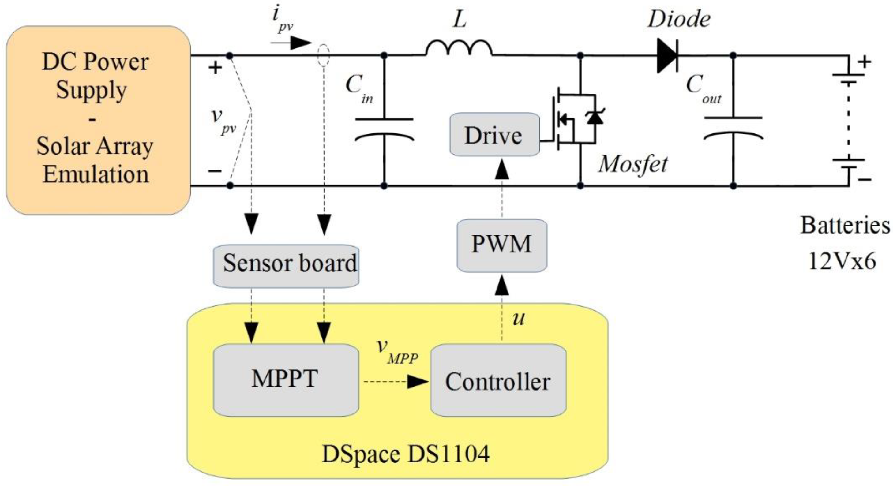
3.2. Case 2: Online Test Using Closed Loop Control

In order to validate the proposed method, an experimental test bench was built considering the elements showed in Figure 2. A Chroma programmable DC Power Supply, model 62050H-600S with Solar Array Emulation capabilities was used as the power source and connected to a dc-dc Boost converter with a rated capability of 350 W. Table 3 contains the main parameters of the power converter. A series connection of six batteries was used as load with 12 volts in each battery. The proposed MPPT algorithm and the closed loop controller were implemented in a DS1104 dSpace digital board with a sampling frequency of 70 kHz. The PWM technique, for the dc–dc converter, was implemented with analog circuits at a frequency of 10 kHz.
Figure 8 shows the simplified diagram of the experimental platform including dc–dc boost converter details. The complete experimental platform is shown in Figure 9 and illustrates the mentioned elements.
It should be noted that the control strategy is based on a previous contribution of the authors and is based on a high-performance input–output linearization controller; details about the controller can be found in [20].
First, three arbitrary points of the PV curve were required as the input information of the proposed algorithm. This can be accomplished with an induced change in the setpoint reference of the closed-loop control. Figure 10a shows two setpoint changes (upper side) and their corresponding PV power (lower side). Its corresponding PV curve is illustrated in Figure 10b. The obtained results are summarized in Table 4 for a solar irradiance of 500 W/m2.
In order to prove that the proposed methodology can be applied under different conditions, another set of points were generated with a solar irradiance of 1000 W/m2. Figure 11a shows the setpoint changes (upper side) and their corresponding PV power (lower side). Its corresponding PV curve is illustrated in Figure 11b. The obtained results are summarized in Table 5.
Notice that in Table 4 and Table 5, the v M P P value was calculated with Equation (10); such an equation involves purely algebraic operations, thus making a very fast algorithm. Another benefit is the absence of a v o c and i s c measurement, making this proposal less invasive than other solutions. This is important because the measurement of v o c or i s c produce a temporal stop of power flow from the PV module to the load. In addition, the arbitrary selected points of the P–V curve were selected according to (1) and (2).
It should be observed that the time between setpoint changes ( t ) in Figure 10 and Figure 11 can be reduced. The employed t was selected only for the validation of the proposed algorithm and to clearly show the proposed method: t 0.25 s .
In real time applications t will be limited by the settling time ( t s ) of the closed-loop controller. This situation is observed in Figure 12, where after the calculation of the new v M P P value and its corresponding actualization, a set point change occurs and t s is required in order to obtain a new measurement under steady-state conditions.
Considering the transient response under a closed-loop controller, the following criteria of t selection is proposed.
t > 2 * t s
In the present experiments, the closed-loop controller allows us to establish t s with the following relationship:
t s = 7 * 1 f s w ,
where f s w stands for the PWM switching frequency on the dc–dc boost converter. More details about the high-performance closed-loop controller can be found in [20].
Based on the previous relationships, the minimum required time to perturb v r e f for taking a new measurement will be
t ( m i n ) = 14 * 1 f s w .
In the experiments, and with f s w = 10 k H z , we have t ( m i n ) = 1.4 m s as the time required to take a new measurement, which is illustrated in Figure 12, where t s = 0.7 m s .
Finally, the flowchart for the proposed method is included in Appendix B. The flowchart shows that the measurement of v O C is only needed at the beginning of the operation. As a starting point, it is suggested that v M P P = 0.8 * v o c and then Q 1 , Q 2 and Q 3 can be measured. Next, by using the proposed method, a new v M P P can be calculated. Then, the update of the voltage reference is applied by making v r e f = v M P P . Note that the flowchart includes a delay time ( t D ); this time is required between each iteration and is a user-defined parameter.

4. Discussion

In this paper, an improved Fractional Open Circuit Voltage (FOCV) MPPT method was presented, which requires only three points of the P–V curve of PV modules. Here, an analytical equation has been proposed in this paper by using the classical circumference equation, thereby allowing the calculation of the voltage at the maximum power point ( v M P P ). This proposal has been validated through numerical and experimental tests by considering a closed-loop operation in the power converter. Furthermore, there is no need for i S C measurement; also, v O C would be required only at the beginning of the day, making it ideal for online applications. Currently, sudden irradiance changes produce changes in i S C and have minimal impact in the v O C value. For this reason, the proposed method can be employed to deal with this phenomenon. In contrast, temperature changes produce a direct impact on the v O C voltage value, just as reported in the literature. For this reason, the proposed method flowchart includes an initial measurement of v O C . However, after the initial measurement of v O C , it is no longer required for the calculation of v M P P . Indeed, the proposed method produces minimal interference between the PV module and the load by avoiding the measurement of i S C and reducing the number of times v O C is measured. Additionally, this proposal copes with the main disadvantage of analytical approaches that require a huge amount of data from manufacturer datasheets. As a final characteristic, the proposed algorithm has very few computational requirements.
Finally, note that the proposed method includes elements of the CF approach. In addition, the present proposal is considered as an improved FOCV method because it uses the same boundaries. However, in comparison with the regular FOCV, the proposed method can be used to calculate a precise value of v M P P .

Author Contributions

Conceptualization and methodology, E.B.-B.; validation, E.B.-B. and D.R.E.-T.; formal analysis, E.B.-B. and D.R.E.-T.; resources, J.A.P.-S.; writing—original draft preparation, E.B.-B.; writing—review and editing, E.B.-B., D.R.E.-T., J.A.P.-S. and H.A.Á.-M.; project administration, Á.A.V.-H. and I.C.-M. All authors have read and agreed to the published version of the manuscript.

Funding

This research received no external funding.

Data Availability Statement

Not applicable.

Conflicts of Interest

The authors declare no conflict of interest.

Appendix A

Table A1. PV module data.
Solartec S72MC-175
VIP
0.535.32.809
15.905.2984.26
18.555.2998.30
21.205.29112.30
23.855.29126.21
26.505.27139.87
28.005.26147.32
30.215.22157.75
32.335.14166.18
34.455.01172.77
35.514.91174.52
36.044.85174.91
36.574.78174.90
37.104.70174.44
39.224.24166.37
40.803.68150.27
41.873.14131.61
42.932.37102.15
43.991.1350.00
44.4000

Appendix B

Figure A1. Suggested flowchart for the proposed method.
Mathematics 11 00526 g0a1

References

  1. Bollipo, R.B.; Mikkili, S.; Bonthagorla, P.K. Hybrid, optimization, intelligent and classical PV MPPT techniques: Review. CSEE J. Power Energy Syst. 2020, 7, 9–33. [Google Scholar] [CrossRef]
  2. Hanzaei, S.H.; Gorji, S.A.; Ektesabi, M. A Scheme-Based Review of MPPT Techniques With Respect to Input Variables Including Solar Irradiance and PV Arrays’ Temperature. IEEE Access 2020, 8, 182229–182239. [Google Scholar] [CrossRef]
  3. Zhang, W.; Zhou, G.; Ni, H.; Sun, Y. A Modified Hybrid Maximum Power Point Tracking Method for Photovoltaic Arrays Under Partially Shading Condition. IEEE Access 2019, 7, 160091–160100. [Google Scholar] [CrossRef]
  4. El-Helw, H.M.; Magdy, A.; Marei, M.I. A Hybrid Maximum Power Point Tracking Technique for Partially Shaded Photovoltaic Arrays. IEEE Access 2017, 5, 11900–11908. [Google Scholar] [CrossRef]
  5. Troudi, F.; Jouini, H.; Mami, A.; Ben Khedher, N.; Aich, W.; Boudjemline, A.; Boujelbene, M. Comparative Assessment between Five Control Techniques to Optimize the Maximum Power Point Tracking Procedure for PV Systems. Mathematics 2022, 10, 1080. [Google Scholar] [CrossRef]
  6. Restrepo, C.; Yanẽz-Monsalvez, N.; González-Castaño, C.; Kouro, S.; Rodriguez, J. A Fast Converging Hybrid MPPT Algorithm Based on ABC and P&O Techniques for a Partially Shaded PV System. Mathematics 2021, 9, 2228. [Google Scholar] [CrossRef]
  7. Wang, S.-C.; Pai, H.-Y.; Chen, G.-J.; Liu, Y.-H. A Fast and Efficient Maximum Power Tracking Combining Simplified State Estimation With Adaptive Perturb and Observe. IEEE Access 2020, 8, 155319–155328. [Google Scholar] [CrossRef]
  8. Bi, Z.; Ma, J.; Man, K.L.; Smith, J.S.; Yue, Y.; Wen, H. An Enhanced 0.8 VOC-Model-Based Global Maximum Power Point Tracking Method for Photovoltaic Systems. IEEE Trans. Ind. Appl. 2020, 56, 6825–6834. [Google Scholar] [CrossRef]
  9. Alsumiri, M. Residual Incremental Conductance Based Nonparametric MPPT Control for Solar Photovoltaic Energy Conversion System. IEEE Access 2019, 7, 87901–87906. [Google Scholar] [CrossRef]
  10. Farah, L.; Hussain, A.; Kerrouche, A.; Ieracitano, C.; Ahmad, J.; Mahmud, M. A Highly-Efficient Fuzzy-Based Controller With High Reduction Inputs and Membership Functions for a Grid-Connected Photovoltaic System. IEEE Access 2020, 8, 163225–163237. [Google Scholar] [CrossRef]
  11. Obukhov, S.; Ibrahim, A.; Zaki Diab, A.A.; Al-Sumaiti, A.S.; Aboelsaud, R. Optimal Performance of Dynamic Particle Swarm Optimization Based Maximum Power Trackers for Stand-Alone PV System Under Partial Shading Conditions. IEEE Access 2020, 8, 20770–20785. [Google Scholar] [CrossRef]
  12. Baimel, D.; Tapuchi, S.; Levron, Y.; Belikov, J. Improved Fractional Open Circuit Voltage MPPT Methods for PV Systems. Electronics 2019, 8, 321. [Google Scholar] [CrossRef] [Green Version]
  13. Ali, A.; Almutairi, K.; Padmanaban, S.; Tirth, V.; Algarni, S.; Irshad, K.; Islam, S.; Zahir, M.H.; Shafiullah, M.; Malik, M.Z. Investigation of MPPT Techniques Under Uniform and Non-Uniform Solar Irradiation Condition–A Retrospection. IEEE Access 2020, 8, 127368–127392. [Google Scholar] [CrossRef]
  14. Pindado, S.; Cubas, J.; Roibás-Millán, E.; Bugallo-Siegel, F.; Sorribes-Palmer, F. Assessment of Explicit Models for Different Photovoltaic Technologies. Energies 2018, 11, 1353. [Google Scholar] [CrossRef] [Green Version]
  15. Ostadrahimi, A.; Mahmoud, Y. Novel Spline-MPPT Technique for Photovoltaic Systems Under Uniform Irradiance and Partial Shading Conditions. IEEE Trans. Sustain. Energy 2021, 12, 524–532. [Google Scholar] [CrossRef]
  16. González-Castaño, C.; Restrepo, C.; Revelo-Fuelagán, J.; Lorente-Leyva, L.L.; Peluffo-Ordóñez, D.H. A Fast-Tracking Hybrid MPPT Based on Surface-Based Polynomial Fitting and P&O Methods for Solar PV under Partial Shaded Conditions. Mathematics 2021, 9, 2732. [Google Scholar] [CrossRef]
  17. Álvarez, J.M.; Alfonso-Corcuera, D.; Roibás-Millán, E.; Cubas, J.; Cubero-Estalrrich, J.; Gonzalez-Estrada, A.; Jado-Puente, R.; Sanabria-Pinzón, M.; Pindado, S. Analytical Modeling of Current-Voltage Photovoltaic Performance: An Easy Approach to Solar Panel Behavior. Appl. Sci. 2021, 11, 4250. [Google Scholar] [CrossRef]
  18. Pindado, S.; Cubas, J. Simple mathematical approach to solar cell/panel behavior based on datasheet information. Renew. Energy 2017, 103, 729–738. [Google Scholar] [CrossRef] [Green Version]
  19. Andrean, V.; Chang, P.; Lian, K. A Review and New Problems Discovery of Four Simple Decentralized Maximum Power Point Tracking Algorithms—Perturb and Observe, Incremental Conductance, Golden Section Search, and Newton’s Quadratic Interpolation. Energies 2018, 11, 2966. [Google Scholar] [CrossRef] [Green Version]
  20. Espinoza, D.; Barcenas, E.; Campos-Delgado, D.; De Angelo, C. Voltage-Oriented Input-Output Linearization Controller as Maximum Power Point Tracking Technique for Photovoltaic Systems. IEEE Trans. Ind. Electron. 2014, 62, 3499–3507. [Google Scholar] [CrossRef]
Figure 1. Photovoltaic I–V and P–V graphs.
Mathematics 11 00526 g001
Figure 2. Typical solution for photovoltaic energy harvesting.
Mathematics 11 00526 g002
Figure 3. P–V curve illustrating the zone of interest.
Mathematics 11 00526 g003
Figure 4. P–V curve with three arbitrary points.
Mathematics 11 00526 g004
Figure 5. Proposed model within the zone of interest.
Mathematics 11 00526 g005
Figure 6. Test Bench for Solartec S72MC-175.
Mathematics 11 00526 g006
Figure 7. v M P P with Solartec S72MC-175.
Mathematics 11 00526 g007
Figure 8. Simplified diagram.
Mathematics 11 00526 g008
Figure 9. Experimental test bench.
Mathematics 11 00526 g009
Figure 10. Three arbitrary points of the PV curve with 500 W/m2. (a) Experimental generation of three points with setpoint changes and (b) location of the three points in the PV curve.
Mathematics 11 00526 g010
Figure 11. Three arbitrary points on the PV curve with 1000 W/m2. (a) Experimental generation of three points with setpoint changes and (b) location of the three points on the PV curve.
Mathematics 11 00526 g011
Figure 12. Transient time response ( t S ) under closed-loop control.
Mathematics 11 00526 g012
Table 1. Numerical evaluation with Solartec S72MC-175.
ParameterValueEquation
Q 1 ( v 1 , p 1 ) Q 1 ( 35.51 , 174.52 ) -
Q 2 ( v 2 , p 2 ) Q 2 ( 36.57 , 174.90 ) -
Q 3 ( v 3 , p 3 ) Q 3 ( 37.10 , 174.44 ) -
( x 1 , y 1 ) (36.04, 174.71)(4)
x 2 , y 2 (36.835, 174.67)(5)
m 11 −2.7894(6)
m 22 1.11521(7)
v M P P 36.28 V(10)
Table 2. Calculated error for v M P P voltage.
Exact v M P P
Calculated   v M P P
Fractional   Method v M P P
Proposed Method
Error (%)
Fractional
Method
Error (%)
36.30 V36.28 VBetween 31.08 V to 39.96 V0.05%14.3% (worst case)
Table 3. Parameters of the dc–dc boost converter.
ParameterValue
MosfetIRFP250N
DiodeSTTH30R04W
L1.5 mH
Cin30 μ F
Cout680 μ F
Table 4. Experimental selected points under an irradiance of 500 W/m2.
PV Module Q 1 ( v 1 , p 1 ) Q 2 ( v 2 , p 2 ) Q 3 ( v 3 , p 3 )
Solar Array Emulator(27.0 V, 73.72 W)(28.0 V, 75.30 W)(31.0 V, 75.55 W)
Calculated v M P P 29.69 V
Exact v M P P 29.73 V
Error %0.13%
Table 5. Experimental selected points under an irradiance of 1000 W/m2.
PV Module Q 1 ( v 1 , p 1 ) Q 2 ( v 2 , p 2 ) Q 3 ( v 3 , p 3 )
Solar Array Emulator(28.00, 146.70)(31.00, 147.70)(32.00, 143.50)
Calculated v M P P 30.14 V
Exact v M P P 30.00 V
Error %0.46%
Disclaimer/Publisher’s Note: The statements, opinions and data contained in all publications are solely those of the individual author(s) and contributor(s) and not of MDPI and/or the editor(s). MDPI and/or the editor(s) disclaim responsibility for any injury to people or property resulting from any ideas, methods, instructions or products referred to in the content.

