Article

Statistical Analysis and Theoretical Framework for a Partially Accelerated Life Test Model with Progressive First Failure Censoring Utilizing a Power Hazard Distribution

by
Amel Abd-El-Monem
1,
Mohamed S. Eliwa
2,3,*,
Mahmoud El-Morshedy
4,5,
Afrah Al-Bossly
4 and
Rashad M. EL-Sagheer
6,7
1
Department of Mathematics, Faculty of Education, Ain-Shams University, Cairo 11566, Egypt
2
Department of Statistics and Operation Research, College of Science, Qassim University, Buraydah 51482, Saudi Arabia
3
Department of Mathematics, Faculty of Science, Mansoura University, Mansoura 35516, Egypt
4
Department of Mathematics, College of Science and Humanities in Al-Kharj, Prince Sattam Bin Abdulaziz University, Al-Kharj 11942, Saudi Arabia
5
Department of Statistics and Computer Science, Faculty of Science, Mansoura University, Mansoura 35516, Egypt
6
Mathematics Department, Faculty of Science, Al-Azhar University, Naser City, Cairo 11884, Egypt
7
High Institute of Computer and Management Information System, First Statement, New Cairo, Cairo 11865, Egypt
*
Author to whom correspondence should be addressed.
Mathematics 2023, 11(20), 4323; https://doi.org/10.3390/math11204323
Submission received: 28 August 2023 / Revised: 9 October 2023 / Accepted: 12 October 2023 / Published: 17 October 2023
(This article belongs to the Special Issue Advances in Applied Probability and Statistical Inference)

Abstract

:
Monitoring life-testing trials for a product or substance often demands significant time and effort. To expedite this process, sometimes units are subjected to more severe conditions in what is known as accelerated life tests. This paper is dedicated to addressing the challenge of estimating the power hazard distribution, both in terms of point and interval estimations, during constant- stress partially accelerated life tests using progressive first failure censored samples. Three techniques are employed for this purpose: maximum likelihood, two parametric bootstraps, and Bayesian methods. These techniques yield point estimates for unknown parameters and the acceleration factor. Additionally, we construct approximate confidence intervals and highest posterior density credible intervals for both the parameters and acceleration factor. The former relies on the asymptotic distribution of maximum likelihood estimators, while the latter employs the Markov chain Monte Carlo technique and focuses on the squared error loss function. To assess the effectiveness of these estimation methods and compare the performance of their respective confidence intervals, a simulation study is conducted. Finally, we validate these inference techniques using real-life engineering data.

1. Introduction

Most manufacturers are currently dedicated to optimizing their product performance to increase demand and establish trust with their customers. However, during the product development process, producers encounter several challenges, including difficulties in managing product failures within the allocated test duration for reliability estimation. In industrial operations, typical operating conditions often result in long periods required to observe unit failures, leading to extended average product failure times. This misalignment with modern industrial practices and technology standards prompted the adoption of accelerated life testing (ALT) by experimenters to expedite responses in such scenarios. ALT involves subjecting the test units to stress levels higher than standard values to accelerate the failure process. Typically, experimenters use data from accelerated tests to estimate the failure distribution of these units. Consequently, there are two categories of ALTs: fully accelerated life tests, where the relationship between life and stress is known, and partially accelerated life tests, where this relationship is either unknown or cannot be assumed. To estimate the lifespan distribution under typical usage conditions, a statistically relevant model is employed to extrapolate data obtained from these accelerated settings.
As outlined by [1], ALT encompasses various stress loading methods, namely constant stress, step stress, and progressive stress. In constant-stress ALT, sample units endure a sustained stress level until they either fail or undergo censoring, whichever occurs first. However, constant-stress testing may become impractical in certain scenarios due to the broad spectrum of failure times. In such cases, there is a need for a method that ensures faster failure occurrence. Step-stress testing, which proves to be more efficient and practical compared to continuous stress, appears to address this issue effectively. In step-stress testing, the test unit is exposed to a specific stress level for a predefined duration until it fails. Should it not fail within this period, the stress level is incrementally increased until the unit eventually fails or reaches the censored condition. In progressive-stress ALT, test units experience continuously increasing stress levels over time. Various researchers have investigated these three stress-loading methods using a variety of distributions (refer to [2,3,4,5,6,7]).
Given the known or assumed relationship between product life and stress, the fundamental presumption in ALT is that data acquired under accelerated conditions can be extrapolated to reflect performance under normal usage conditions. Nevertheless, it has been observed that, in certain situations, particularly when dealing with new test units, it becomes challenging to ascertain or make a reliable assumption about this relationship. Consequently, in such cases, partial accelerated life tests (PALT) are frequently employed. PALT finds its utility in test environments where it is challenging to collect lifetimes for highly reliable items with extended lifespans using conventional test conditions. PALT typically falls into two distinct categories: step-stress PALT (SS-PALT) and constant-stress PALT (CS-PALT). In CS-PALT, all groups of test units are individually exposed to accelerated conditions and usage profiles. Conversely, in SS-PALT, the usage conditions for the remaining components of the experiment transition from normal use to higher stress levels at predetermined times or after a predefined number of failures. Recent research in the field of PALT has yielded numerous studies, some of which are exemplified by references [8,9,10,11,12,13,14].
While the primary objective of PALT is to shorten the duration of the testing experiment, experimenters often face substantial downtime as they wait for all test units to fail. To mitigate this challenge, working with censored data becomes essential, aiming to reduce both the cost and duration of the test. Two commonly employed types of censorship are type-I and type-II censoring. In the former, units are simultaneously tested for a predetermined duration, and during this period, some units experience failure; subsequently, the remaining units are withdrawn from the test at its conclusion (refer to [15,16]). Conversely, in the latter, units are tested concurrently until a predefined number of failures occur, at which point the remaining units are removed (as described in [17]). However, these earlier approaches lack flexibility in terms of removing test units mid-test. To address this limitation, a progressive type-II censoring (PTIIC) scheme is proposed as a more versatile censoring method to overcome this challenge. In PTIIC, predetermined units are removed from the test at the moment of a single unit’s failure, and the test proceeds at this pace until a fixed number of units experience failure. Upon reaching this point (the last failed unit), the remaining surviving units are then removed (refer to [18,19,20]).
At times, the duration of the control experiment can become excessively long due to product aging issues. A life test method introduced by [21] offers experimenters the flexibility to segregate the test units into distinct groups and simultaneously run each group until the first failure occurs within each group. This form of censorship is referred to as ‘first-failure censoring’. However, under this censoring approach, the researcher cannot remove experimental groups from the test until the first failure is observed. To address this limitation, ref. [22] devised a life testing approach that combines first-failure censoring with progressive type-II censoring, resulting in what is known as a ‘progressive first-failure censoring’ (PFFC) scheme, which will be discussed in the upcoming section. Let us now briefly delve into the progressive first-failure filtering system. Let us put n-independent groups each with k units to the test in real life. Start removing R 1 number of groups as soon as X 1 : m : n : k encounters its first failure. Repeat after the second failure time X 2 : m : n : k , deleting R 2 groups at random from the experiment as well as the group where the second failure was noticed. The experimenter keeps going in the same way until all live R m groups that are still active and the group where the m t h failure has taken place have been eliminated. The observed failures X 1 : m : n : k < X 2 : m : n : k < < X m : m : n : k are referred to as progressive first failure censored order statistics, whereas the progressive censoring scheme is known as R = ( R 1 , , R m ) . Recent years have seen an increase in the amount of literature on PFFC, including in [23,24,25,26,27,28,29,30].
In the realm of lifetime data analysis and the modeling of failure processes, parametric models play a crucial role and are widely employed due to their demonstrated utility across diverse scenarios. Among the various univariate models, a select few distributions hold a prominent position for their proven effectiveness in a wide array of situations. Notably, the exponential, Weibull, gamma, and log-normal distributions stand out in this regard. Another versatile model for lifetime distribution, capable of fitting well with certain sets of failure data, is the power hazard function distribution (PHFD). Reference [31] delved into the application of the PHFD and illustrated its suitability for assessing the reliability of electrical components. Through analyses of reliability and hazard functions, they demonstrated that the PHFD outperforms the exponential, log-normal, and Weibull distributions in this context. As an alternative to the Weibull, Rayleigh, and exponential distributions, Reference [32] explored the two-parameter version of PHFD, denoted as PHFD( δ , ρ ), and investigated its various characteristics. If X is a continuous random variable that obeys a PHFD with shape and scale parameters δ and ρ , respectively, the probability density function (PDF) and its related cumulative distribution function (CDF) can be written as
f x ; δ , ρ = ρ x δ exp ρ δ + 1 x δ + 1 , x > 0 ,
and
F x ; δ , ρ = 1 exp ρ δ + 1 x δ + 1 , x > 0 ,
respectively. Additionally, the failure rate (FR) and survival functions (SF) can be represented as
h x ; δ , ρ = ρ x δ , x > 0 ,
and
S x ; δ , ρ = exp ρ δ + 1 x δ + 1 , x > 0 ,
where ρ > 0 , and δ > 1 . When δ > 0 , this distribution’s FR function increases, and when 1 < δ < 0 , it decreases. This distribution is a very adaptable model, and when its parameters are altered, it approaches various models. It includes the following specific models: PHFD relates to Rayleigh( α ) when ρ = 1 / α 2 and δ = 1 , PHFD lowers to Weibull( ρ , 1 ) when δ = ρ 1 , and PHFD is an exponential distribution with mean 1 / ρ when δ = 0 . Because of these characteristics, this model was utilized by multiple writers to model data, particularly censored observations. Due to its practical significance in the wide range of alternative fields, as noted in numerous references, this distribution’s verification throughout this work serves as our inspiration. These references include in [33,34,35,36,37].
The paper is structured and organized as follows: Section 2 introduces the model description and lays out the fundamental assumptions. In Section 3, we delve into the most common estimations, including maximum likelihood estimates (MLEs) and the construction of approximate confidence intervals for unknown parameters. Section 4 is dedicated to the discussion of percentile bootstrap and bootstrap-t algorithms. Section 5 outlines the process of generating Bayes point estimates using the squared error loss function and provides insights into the associated credible intervals. In Section 6, we conduct a simulation study using Monte Carlo methods. Section 7 illustrates the application of our methodology with a real engineering example. Finally, Section 8 presents some concluding remarks.

2. Model Descriptions and Assumptions

PALT is often employed in testing scenarios where it is challenging to collect data on the lifetimes of exceptionally reliable units with long lifespans under typical testing conditions. In PALT, certain test units are subjected to elevated stress levels, while others are placed in a standard testing environment. This study specifically focuses on the CS-PALT criterion, where some test units operate under normal stress conditions, while others are subjected to a continuous elevated stress level.

2.1. Model Description

As previously mentioned, in CS-PALT, N 1 test units are randomly chosen from the total number of units available N, and they are run under normal conditions, while the remaining N 2 = N N 1 test units are operated under accelerated settings. Assuming the test unit’s lifespan complies with the PHFD, the PDF, CDF, and FR function under typical circumstances are provided, respectively, by
f 1 x 1 ; δ , ρ = ρ x 1 δ exp ρ δ + 1 x 1 δ + 1 , x 1 > 0 ,
F 1 x 1 ; δ , ρ = 1 exp ρ δ + 1 x 1 δ + 1 , x 1 > 0 ,
and
h 1 x 1 ; δ , ρ = ρ x 1 δ , x 1 > 0 ,
where ρ > 0 , and δ > 1 . When a unit is tested under accelerated conditions, the FR function is provided by the formula
h 2 x 2 ; β , δ , ρ = β h 1 ( x 1 ) = β ρ x 2 δ , x 2 > 0 ,
where β is an acceleration factor that meets the criterion β > 1 . As a result, the SF, CDF, and PDF may each be expressed as follows
S 2 x 2 ; β , δ , ρ = exp β ρ δ + 1 x 2 δ + 1 , x 2 > 0 ,
F 2 x 2 ; β , δ , ρ = 1 exp β ρ δ + 1 x 2 δ + 1 , x 2 > 0 ,
and
f 2 x 2 ; β , δ , ρ = β ρ x 2 δ exp β ρ δ + 1 x 2 δ + 1 , x 1 > 0 .
Figure 1 plots the PDFs under normal and accelerated conditions. In this instance, CS-PALT and PFFC are coupled. As a result, Group 1 and Group 2 will be created from the entire N test units. The first group’s components ( N 1 = n 1 k 1 ) are categorized as belonging to normal conditions, whereas the second group’s components ( N 2 = n 2 k 2 ) are categorized as belonging to stress conditions. Each group is split into a number of groups with k j , j = 1 , 2 test units under either normal or accelerated settings. The progressive censoring plans for the normal and accelerated tests in this approach are R 1 i and R 2 i , respectively. This technique continues to operate until m j , where j = 1 , 2 failures are noticed in each test condition. The likelihood function of the observed sample of PFFC scheme under CS-PALT can be expressed as follows:
L ( β , δ , ρ | x ̲ ) i = 1 m 1 f 1 x 1 i ; δ , ρ 1 F 1 x 1 i ; δ , ρ k 1 R 1 i + 1 1 × i = 1 m 2 f 2 x 2 i ; β , δ , ρ 1 F 2 x 2 i ; β , δ , ρ k 2 R 2 i + 1 1 .

2.2. Assumptions

These presumptions are made in relation to the proposed PALT methodology:
  • The lifetime of all units tested under various normal or accelerated conditions follows the PHFD.
  • The lifetimes of test units are independent identically distributed random variables.
  • The total number of units under test is N = N 1 + N 2 = n 1 k 1 + n 2 k 2 .
  • Any unit has a lifetime of X 2 = β 1 X 1 under accelerated conditions.
  • The lifetimes X 1 i , i = 1 , 2 , , m 1 of units assigned to the normal condition, while the lifetimes X 2 i , i = 1 , 2 , , m 2 of units assigned to the accelerated condition are independent of one another.

3. Maximum Likelihood Estimation

One of the most significant and popular statistical techniques is the maximum likelihood estimate (MLE). The maximum likelihood (ML) technique produces estimates of parameters with favorable statistical properties, such as consistency, asymptotic unbiasedness, asymptotic efficiency, and asymptotic normality. To obtain the parameter estimates with the maximum likelihood, one must calculate the estimates of the parameter that maximizes the probability of the sample data. The MLEs are consistent and asymptotically normal for large samples, which are other desired characteristics. Let X j 1 : m j : n j : k j R j < X j 2 : m j : n j : k j R j < < X j m j : m j : n j : k j R j for j = 1 , 2 represent the two PFFC samples from the two populations whose PDFs and CDFs are as indicated in (1), (2), and (6), (7) with censoring scheme R j = ( R j 1 , R j 2 , , R j m ) . Without a normalized constant, the logarithm likelihood function can be written as
( β , δ , ρ | x ̲ ) m 1 + m 2 log ρ + m 2 log β + δ i = 1 m 1 log x 1 i + i = 1 m 2 log x 2 i ρ Φ 1 + β Φ 2 ,
where
Φ s = 1 δ + 1 i = 1 m s k s R s i + 1 x s i δ + 1 , s = 1 , 2 .
By computing the first derivatives of (9) with respect to β , δ , and ρ and then setting them equal to zero, the resulting simultaneous equations are represented as follows
( β , δ , ρ | x ̲ ) β = m 2 β ρ Φ 2 = 0 ,
( β , δ , ρ | x ̲ ) δ = i = 1 m 1 log x 1 i + i = 1 m 2 log x 2 i ρ Φ 3 Φ 1 δ + 1 + β Φ 4 Φ 2 δ + 1 = 0 ,
where
Φ t = 1 δ + 1 i = 1 m t k t R t i + 1 x t i δ + 1 log x t i , t = 3 , 4 ,
and
( β , δ , ρ | x ̲ ) ρ = m 1 + m 2 ρ Φ 1 + β Φ 2 = 0 .
A system of three non-linear equations in three unknowns β , δ , and ρ are formally represented by the equations that come before them. The previous non-linear equations are challenging to provide closed-form solutions to theoretically. In order to obtain the MLEs ( β ^ M L , δ ^ M L , ρ ^ M L ) of β , δ , ρ , the numerical Newton–Raphson approach will be used to solve these simultaneous equations to obtain the estimates. The algorithm is described as follows:
(1)
Use the method of moments or any other methods to estimate the parameters β ,   δ and ρ as starting point of iteration, denote the estimates as β 0 , δ 0 , ρ 0 , and set l = 0 .
(2)
Calculate β , δ , ρ β l , δ l , ρ l and the observed Fisher information matrix I 1 β , δ , ρ , given in Section 3.
(3)
Update β , δ , ρ as
β l + 1 , δ l + 1 , ρ l + 1 = β l , δ l , ρ l + β , δ , ρ β l , δ l , ρ l × I 1 β , δ , ρ .
(4)
Set l = l + 1 , and then go back to Step (1).
(5)
Continue the iterative steps until β l + 1 , δ l + 1 , ρ l + 1 β l , δ l ,   ρ l is smaller than a threshold value. The final estimates of β ,   δ , and ρ are the MLE of the parameters, denoted as β ^ ,   δ ^ and ρ ^ .
To delve deeper into the topic, refer to [20] for additional information. For distributions that are expressed using more than one parameter, the second derivatives are crucial for a number of reasons. They will confirm that maxima have been found for one of those reasons. The second partial derivatives of the likelihood function in our situation can be written as
2 ( β , δ , ρ | x ̲ ) β 2 = m 2 β 2 ,
2 ( β , δ , ρ | x ̲ ) β δ = 2 ( β , δ , ρ | x ̲ ) δ β = ρ Φ 4 Φ 2 δ + 1 ,
2 ( β , δ , ρ | x ̲ ) β ρ = 2 ( β , δ , ρ | x ̲ ) ρ β = Φ 2 ,
2 ( β , δ , ρ | x ̲ ) ρ 2 = m 1 + m 2 ρ 2 ,
( β , δ , ρ | x ̲ ) ρ δ = ( β , δ , ρ | x ̲ ) δ ρ = Φ 3 Φ 1 δ + 1 β Φ 4 Φ 2 δ + 1 ,
and
2 ( β , δ , ρ | x ̲ ) δ 2 = 2 ρ δ + 1 Φ 3 Φ 1 + β Φ 4 Φ 2 ρ Φ 5 β Φ 6 ,
where
Φ v = 1 δ + 1 i = 1 m v k v R v i + 1 x v i δ + 1 log x v i 2 , v = 5 , 6 .
The Fisher information matrix (FIM) is obtained by arranging the second partial derivatives (15)–(20) in a matrix structure. The FIM being negative semi-definite is a necessary requirement in an optimization context for a stationary point to be a maximum. The asymptotic variances–covariances of the maximum likelihood estimators β ^ M L ,   δ ^ M L , and ρ ^ M L of the parameters β ,   δ and ρ are obtained by the elements of the inverse of the FIM. The observed asymptotic variance-covariance matrix for the ML estimators is obtained as
I 1 ( β , δ , ρ ) = 2 ( β , δ , ρ | x ̲ ) β 2 2 ( β , δ , ρ | x ̲ ) β δ 2 ( β , δ , ρ | x ̲ ) β ρ 2 ( β , δ , ρ | x ̲ ) δ β 2 ( β , δ , ρ | x ̲ ) δ 2 ( β , δ , ρ | x ̲ ) δ ρ 2 ( β , δ , ρ | x ̲ ) ρ β ( β , δ , ρ | x ̲ ) ρ δ 2 ( β , δ , ρ | x ̲ ) ρ 2 ( β ^ M L , δ ^ M L , ρ ^ M L ) 1 = V a r ( β ^ M L ) C o v ( β ^ M L , δ ^ M L ) C o v ( β ^ M L , ρ ^ M L ) C o v ( δ ^ M L , β ^ M L ) V a r ( δ ^ M L ) C o v ( δ ^ M L , ρ ^ M L ) C o v ( ρ ^ M L , β ^ M L ) C o v ( ρ ^ M L , δ ^ M L ) V a r ( ρ ^ M L ) .
Therefore, using the asymptotic normality of the ML findings of intervals determined, the approximate ( 1 α ) 100 % confidence intervals (ACIs) for β , δ , and ρ are obtained according to
β ^ M L z α 2 V a r ( β ^ M L ) , δ ^ M L z α 2 V a r ( δ ^ M L ) , ρ ^ M L z α 2 V a r ( ρ ^ M L ) .
Here, z α 2 is the percentile of the conventional normal model with a right-tail probability of α 2 . The problem with applying a normal approximation of the MLE is that when the sample size is small, the normal approximation may be poor. However, a different transformation of the MLE can be used to correct the inadequate performance of the normal approximation. Reference [38] presented a log-transformation as a way to enhance the performance of the normal approximation. Therefore, for the parameters being considered, ACIs of ( 1 α ) 100 % are provided as
β ^ M L exp z α 2 V a r ( β ^ M L ) β ^ M L , δ ^ M L exp z α 2 V a r ( δ ^ M L ) δ ^ M L , ρ ^ M L exp z α 2 V a r ( ρ ^ M L ) ρ ^ M L .

3.1. Consistent and Asymptotically Normal Estimators

3.1.1. Consistency characteristic

Consider θ = β , δ , ρ as the true parameter value of a statistical model, and let θ ^ represent the MLE of θ . The MLE is considered consistent when θ ^ converges to θ in probability as the sample size n grows. To establish the MLE’s consistency, we can employ the following theorem.
Theorem 1.
Assuming that the log-likelihood function ( θ | x ̲ ) exhibits continuity with respect to θ and meets the subsequent criteria:
1. 
( θ | x ̲ ) is differentiable in θ for all x in the sample space.
2. 
The expected value of the score function Ω x ̲ , θ = ( θ | x ̲ ) θ is zero at the true parameter value, i.e., E Ω x ̲ , θ = 0 for θ = θ 0 .
3. 
The FIM I 1 θ = E Ω x ̲ , θ Ω x ̲ , θ T is positive definite at the true parameter value, i.e., I 1 θ 0 > 0 .
Then, the θ ^ is a consistent estimator of θ.
Proof. 
Consider ε > 0 as any chosen positive value. Applying the Chebyshev inequality, we obtain
P θ ^ θ > ϵ V a r θ ^ ε 2 .
Utilizing the central limit theorem, it’s established that the distribution of θ ^ tends toward a normal distribution with a mean of θ and a variance of I 1 θ as the sample size n grows. Consequently, we can express this as
V a r θ ^ = I 1 θ + o 1 ,
where o 1 is a term that goes to zero as n increases. Substituting this into the Chebyshev inequality, we obtain
P θ ^ θ > ϵ I 1 θ + o 1 ε 2 .
As the sample size n increases, the term o ( 1 ) diminishes to zero, and the denominator in the inequality grows towards infinity. Consequently, the probability of θ ^ θ > ε approaches zero, thereby confirming the consistency of the θ ^ with respect to θ . □

3.1.2. Asymptotic Normality Characteristic

We describe the θ ^ as exhibiting asymptotic normality when its distribution approximates a normal distribution with a mean of θ and a variance of I 1 θ as the sample size n grows. To establish the MLE’s asymptotic normality, we can utilize the following theorem.
Theorem 2.
If the log-likelihood function ( θ | x ̲ ) fulfills the conditions outlined in the consistency theorem mentioned earlier, then the θ ^ demonstrates asymptotic normality.
Proof. 
According to the central limit theorem, it is established that the distribution of the score function Ω x ̲ , θ tends towards a normal distribution with a mean of zero and a variance of I 1 θ as the sample size n grows. As a result, we can express it as follows:
Ω x ̲ , θ = N 0 , I 1 θ + o 1 ,
here, o ( 1 ) represents a term that diminishes to zero with the increasing value of n. Utilizing the Taylor series expansion, we can express this as
θ ^ θ = I 1 θ Ω x ̲ , θ + o 1 .
Replacing the preceding equation into the score function’s asymptotic normality, we obtain
θ ^ θ = I 1 θ N 0 , I 1 θ + o 1 .
This demonstrates that as the sample size n increases, the distribution of θ ^ θ tends toward a normal distribution with a mean of zero and a variance of I 1 θ , thereby confirming the asymptotic normality of the θ ^ . It is essential to emphasize that the consistency and asymptotic normality properties of MLEs are valid under specific regularity conditions. While these conditions are generally met in numerous statistical models, it is crucial to verify their satisfaction before employing the MLE approach. □

4. Parametric Bootstrap

As mentioned earlier, normal approximations are effective when dealing with large sample sizes. However, when working with small sample sizes, the assumption of normality may not hold. In such cases, the use of resampling techniques like bootstrapping can provide more precise approximations for confidence intervals. Bootstrapping has gained popularity in recent times due to its capability to offer a robust and accurate means of assessing the reliability of a specific model. Bootstrapping entails repeatedly resampling data from a population to obtain more accurate estimates of the population’s true mean and variance. To achieve this, we recommend employing confidence intervals based on two parametric bootstrap methods: the percentile bootstrap technique (Boot-p), which relies on the theory of [39], and the bootstrap-t method (Boot-t), which is grounded in the theory of [40]. To generate bootstrap samples for both approaches, the following procedures are employed:
  • Using the original PFFC sample as a foundation, x j 1 : m j : n j : k j R j , x j 2 : m j : n j : k j R j , , x j m j : m j : n j : k j R j for j = 1 , 2 , obtain β ^ M L ,   δ ^ M L and ρ ^ M L .
  • Employ the censoring plan n j , m j , k j , R j i and ( β ^ M L , δ ^ M L , ρ ^ M L ) to generate a PFFC bootstrap sample x j 1 : m j : n j : k j R j , x j 2 : m j : n j : k j R j , , x j m j : m j : n j : k j R j for j = 1 , 2 .
  • From x j 1 : m j : n j : k j R j , x j 2 : m j : n j : k j R j , , x j m j : m j : n j : k j R j calculate the bootstrap estimates, which are indicated by the symbol η ^ , where η ^ = β ^ M L ,   δ ^ M L and ρ ^ M L .
  • Steps 2 and 3 should be repeated N B times to produce η ^ 1 , η ^ 2 , , η ^ N B .
  • Sort η ^ j ,   j = 1 , 2 , , N B , ascendingly as η ^ j ,   j = 1 , 2 , , N B .

4.1. Parametric Boot-p

Let φ 1 z = P η ^ z be the CDF of η ^ . Define η ^ b o o t p z = φ 1 z for given z. Then, the approximate 100 1 α % Boot-p CI of η ^ is given by
η ^ b o o t p α 2 , η ^ b o o t p 1 α 2 .

4.2. Parametric Boot-t

We discover the ordering statistics η ^ as
ϑ ^ η = η ^ η ^ V a r ( η ^ ) ,
where V a r ( η ^ ) obtained using FIM for η ^ = β ^ M L ,   δ ^ M L and ρ ^ M L . Let φ 2 z = P ϑ ^ η z be the CDF of ϑ ^ η . For a given z, define
η ^ b o o t t z = η ^ + V a r ( η ^ ) φ 2 1 z .
Thus, the approximate 100 1 α % Boot-t CI of η ^ is given by
η ^ b o o t t α 2 , η ^ b o o t t 1 α 2 .

5. Bayesian Estimation

Bayesian estimation is a powerful technique for determining unknown parameters from measurable data. Its foundation is the Bayes theorem, a concept in probability theory that allows the probability of a hypothesis to be updated as new information is gathered. This approach provides a number of benefits over traditional MLE strategies because it may account for prior knowledge while estimating. It also has the ability to assess the degree of uncertainty surrounding each parameter. For Bayesian deduction to work, the priors for the parameters must be chosen correctly. The authors of Reference [41] argue that it is evident that from a properly Bayesian standpoint, one cannot assert that one prior is superior to all others. One must undoubtedly accept their own subjective past with all of its flaws. However, if we have enough information about the parameter(s), employing informative priors that are unquestionably preferred over all other options is preferable. If not, using ambiguous or non-descriptive priors may be appropriate; for more details, see [42]. The family of gamma distributions is known to be simple and flexible enough to suit a variety of the experimenter’s preexisting ideas, according to [43]. Consider the case in which the unknown parameters, δ and ρ , are stochastically independent and have conjugate gamma priors. Specifically, gamma ( a 1 , b 1 ) and gamma ( a 2 , b 2 ) . Additionally, a vague prior is selected for the acceleration factor β with the following PDF
π β = 1 β , β > 0 .
As a result, the joint prior of the parameters δ , ρ , and β together can be stated as follows
π ( β , δ , ρ ) δ a 1 1 ρ a 2 1 β 1 exp b 1 δ b 2 ρ .
In order to present the joint posterior distribution of δ , ρ , and β , one must combine the joint prior distribution π ( β , δ , ρ ) in (38) with the likelihood function L ( β , δ , ρ | x ̲ ) supplied in (8) as
π ( β , δ , ρ | x ̲ ) = L ( β , δ , ρ | x ̲ ) × π ( β , δ , ρ ) 1 0 0 L ( β , δ , ρ | x ̲ ) × π ( β , δ , ρ ) d β d δ d ρ β m 2 1 δ a 1 1 ρ m 1 + m 2 + a 2 1 exp δ b 1 ρ Φ 1 + β Φ 2 + b 2 i = 1 m 1 x 1 i δ i = 1 m 2 x 2 i δ ,
where Φ 1 and Φ 2 are given in (10). In the Bayes technique, one should select a loss function that corresponds to each of the potential estimators in order to arrive at the best estimator. Here, the squared error loss function estimations, which we can express as φ η ^ , η = η ^ η 2 , and Bayes estimate E η η | x ̲ are calculated. The inability to derive the joint posterior in a closed form, which would allow us to compute Bayes estimates of the unknown parameters δ , ρ , and β , may be seen in relation (29). The MCMC technique, which enables us to acquire simulated samples from the posterior distributions of the parameters, will therefore be used in order to obtain these estimations. Calculations for the point and interval estimate of unidentified parameters will be made using these generated samples. As for how this approach operates, it is based on the calculation of conditional posterior functions, where the conditional distribution of β given δ and ρ can be represented as
π 1 ( β | δ , ρ , x ̲ ) β m 2 1 exp β ρ Φ 2 G a m m a m 2 , ρ Φ 2 .
Similarly, the conditional distribution of δ given β and ρ can be reported as
π 2 ( δ | β , ρ , x ̲ ) i = 1 m 1 x 1 i δ i = 1 m 2 x 2 i δ δ a 1 1 exp δ b 1 ρ Φ 1 + β Φ 2 .
Additionally, the conditional distribution of ρ given β and δ can be stated as
π 3 ( ρ | β , δ , x ̲ ) ρ m 1 + m 2 + a 2 1 exp ρ Φ 1 + β Φ 2 + b 2 G a m m a m 1 + m 2 + a 2 , Φ 1 + β Φ 2 + b 2 .
Gamma densities π 1 ( β | δ , ρ , x ̲ ) and π 3 ( ρ | β , δ , x ̲ ) are evident. As a result, samples of β and ρ can be produced using a gamma generator. Additionally, π 2 ( δ | β , ρ , x ̲ ) cannot be reduced for directly drawing samples using conventional techniques. The gamma distribution was chosen as the prior distribution of the parameters because it is the most appropriate one that matches the maximum likelihood function. Moreover, they are from the same family. The evidence for this is that two of the full conditional posterior distributions of the parameters π 1 ( β | δ , ρ , x ̲ ) and π 3 ( ρ | β , δ , x ̲ ) resulted in a gamma distribution, which proves the validity of the choice. In addition, choosing another prior distribution or dependent prior will increase the complexity and difficulty of mathematical equations. Gamma distribution is one of the rich distributions, as when changing its parameters (hyper-parameters), we obtain new data with new information, so it is the focus of attention of most statisticians. A special case is that when all hyper-parameters of gamma distribution are zero, we obtain the Jaffrey prior in the form 1 β , 1 δ , and 1 ρ .
In this scenario, we can utilize the Metropolis–Hastings (M-H) algorithm model, which is suggested by [44], to derive Bayes’ estimate for using one of the well-known MCMC methods. To reduce the rejection rate as much as feasible in this algorithm, we can select either a symmetric or non-symmetric proposal distribution. The normal distribution is included as a symmetric proposal distribution since the marginal distribution of δ is not well known. The M-H steps are additionally incorporated into the Gibbs sampler to update δ , while β as well as ρ is updated straight from its full conditional; see [45] as follows:
  • Start with an ( β , δ , ρ ) = ( β ^ M L , δ ^ M L , ρ ^ M L ) , and set J = 1 .
  • Generate β J from G a m m a m 2 , ρ J 1 Φ 2 .
  • Generate δ J according to the following:
    (a)
    Generate δ from normal distribution N δ J 1 , V a r ( δ ^ M L ) where V a r ( δ ^ M L ) the variance of δ given in (22).
    (b)
    Compute r = min 1 , π 2 ( δ | β J , ρ J 1 , x ̲ ) π 2 ( δ J 1 | β J , ρ J 1 , x ̲ ) .
    (c)
    Generate a sample μ from the U 0 , 1 distribution.
    (d)
    If μ r set δ J = δ ; otherwise, δ J = δ J 1 .
  • Generate ρ J from G a m m a m 1 + m 2 + a 2 , Φ 1 + β J Φ 2 + b 2 .
  • Set J = J + 1 .
  • To collect the required number of samples, repeat Steps 2–5 M times.
The original M 0 sample count from the burn-in process is discarded, and we use the M M 0 samples that are still there to derive estimations. As a result, the Bayes estimate of ζ = ( β , δ   o r   ρ ) under the squared error loss function can be viewed as the average of the samples that were obtained from the posterior densities as follows:
ζ ^ B S = 1 M M 0 J = M 0 + 1 M ζ J .
In order to create the highest posterior density (HPD) credible intervals (CRIs) of ζ = ( β , δ   o r   ρ ) using generated MCMC sampling procedure, we first refer to the ordered random sample produced by the previous algorithm in the form ζ 1 < ζ 2 < < ζ M . Then, the 100 1 α % two-sided CRIs of ζ can be constructed as
ζ ^ M M 0 α 2 , ζ ^ M M 0 1 α 2 .

6. Simulation Study

In this section, some computations in line with Monte Carlo simulation experiments are carried out using Mathematica ver. 13 in an effort to assess the performance of the offered approaches. In light of the proposed algorithm proposed in [18] with the distribution function 1 1 F x k , 1000 PFFC samples were generated under both normal and acceleration conditions from the PHF δ , ρ and PHF β , δ , ρ distributions, respectively, with the parameters β , δ , ρ = ( 2 , 1.5 , 2.5 ) . The effectiveness of the obtained estimates of β , δ , and ρ from the various proposed approaches (MLE, two parametric bootstrap, and MCMC technique) is compared in terms of point and interval estimates. In order to achieve this, mean squared errors (MSEs) are taken into account for point estimates, whereas the average widths (AWs) of 95 % confidence/HPD credible intervals and 95 % coverage probabilities (CPs) of the parameters based on the simulation are taken into account for interval estimates. For the purpose of conducting our investigation, multiple combinations of k 1 = k 2 = k (group size), n 1 = n 2 = n (number of groups), and m j ,   j = 1 , 2 (observed data) are taken into consideration with various censoring schemes (CSs) R j , j = 1 , 2 . For ease, three categories of CSs are taken into consideration, namely R j = ( R j 1 , R j 2 , , R j m )
CS I : R j 1 = n j m j , R j 2 = R j 3 = = R j m j = 0 , j = 1 , 2 . CS II :     R j m j + 1 2 = n j m j , R j i = 0 , for i m j + 1 2 if m j is odd         R j m j 2 = n j m j , R j i = 0 , for i m j 2 if m j is even . CS III : R j 1 = R j 2 = = R j m j 1 = 0 , R j m j = n j m j , j = 1 , 2 .
To resolve the non-linear Equations (11)–(14) and obtain the MLEs of the parameter values, we used the NMaximize command of the Mathematica 13 package. Additionally, the β ^ M L ,   δ ^ M L , and ρ ^ M L are produced utilizing the MLE’s invariance feature. A total of 1000 replicates were used in the investigation. Each replication makes use of 1000 bootstrap (Boot-p and Boot-t) samples. The first 2000 values are deleted as “burn-in” while computing Bayes estimates (BEs) and highest posterior density CRIs in a Bayesian framework utilizing 12,000 MCMC samples. Furthermore, we take into account informative gamma priors with the following hyper-parameter values: a 1 = 2 ,   b 1 = 1 ,   a 2 = 3 , and b 2 = 2 . The parameter values for the informative priors are chosen such that their mean is equal to the parameter values themselves. Table 1, Table 2, Table 3, Table 4 and Table 5 show the outcomes of the Monte Carlo simulation study. These tables allow us to draw the following conclusions:
  • In every instance, as would be expected, the MSEs and AWs of all estimates decrease as sample sizes increase. It verifies the consistency features of each estimation method.
  • With n and m keeping invariant, k increases both MSEs and AWs increase.
  • In terms of decreased MSEs and AWs, the first scheme (I) performs the best when sample sizes are fixed and failures are observed.
  • The MSE and AW both increase when removals are delayed.
  • In terms of MSEs and AWs, Bayes estimation using MCMC performs better than the other approaches (ML, Boot-p, Boot-t).
  • Due to having the smallest MSE and narrowest width, MCMC CRIs are, overall, the most satisfactory.
  • Bootstrap methods outperform the ML approach in terms of MSEs and AWs. Furthermore, Boot-t performs better than Boot-p in terms of MSEs and AWs.
  • The estimates produced by the ML, bootstrap, and Bayesian approaches are highly similar and have high CPs (around 0.95 ).
  • In spite of the fact that the Bayes estimators perform better than all other estimators, the simulation results show that all point and interval estimator approaches are efficient. The Bayes technique may be chosen if one has sufficient prior knowledge. If past knowledge of the topic being studied cannot be accessed, bootstrap approaches that primarily rely on MLEs are preferred.

7. Practical Analysis of Engineering Data

In this section, we want to see how the estimate algorithms suggested for the accelerated data set perform as described in the aforementioned sections. The effectiveness of the suggested inferential approaches is displayed and demonstrated using a genuine data set that represents the observed failure rates in a life test of the light-emitting diode (LED). References [46,47] recently conducted an analysis of this data that was initially conducted by [48]. The observed failure samples were created in both normal and accelerated conditions, and they include the following:
  • Normal use condition: 0.18, 0.19, 0.19, 0.34, 0.36, 0.40, 0.44, 0.44, 0.45, 0.46, 0.47,0.53, 0.57, 0.57, 0.63, 0.65, 0.70, 0.71, 0.71, 0.75, 0.76, 0.76, 0.79,0.80, 0.85, 0.98, 1.01, 1.07, 1.12, 1.14, 1.15, 1.17, 1.20, 1.23, 1.24,1.25, 1.26, 1.32, 1.33, 1.33, 1.39, 1.42, 1.50, 1.55, 1.58, 1.59, 1.62, 1.68, 1.70, 1.79, 2.00, 2.01, 2.04, 2.54, 3.61, 3.76, 4.65, 8.97.
  • Accelerated stress condition: 0.13, 0.16, 0.20, 0.20, 0.21, 0.25, 0.26, 0.28, 0.28, 0.30, 0.31, 0.33, 0.35, 0.35, 0.35, 0.39, 0.50, 0.52, 0.58, 0.60, 0.60, 0.62, 0.63, 0.67, 0.71, 0.73, 0.75, 0.75, 0.78, 0.80, 0.80, 0.86, 0.90, 0.91, 0.93, 0.93, 0.94, 0.98, 0.99, 1.01, 1.03, 1.06, 1.06, 1.10, 1.22, 1.22, 1.24, 1.28, 1.39, 1.39, 1.46, 1.48, 1.52, 1.74, 1.95, 2.46, 3.02, 5.16.
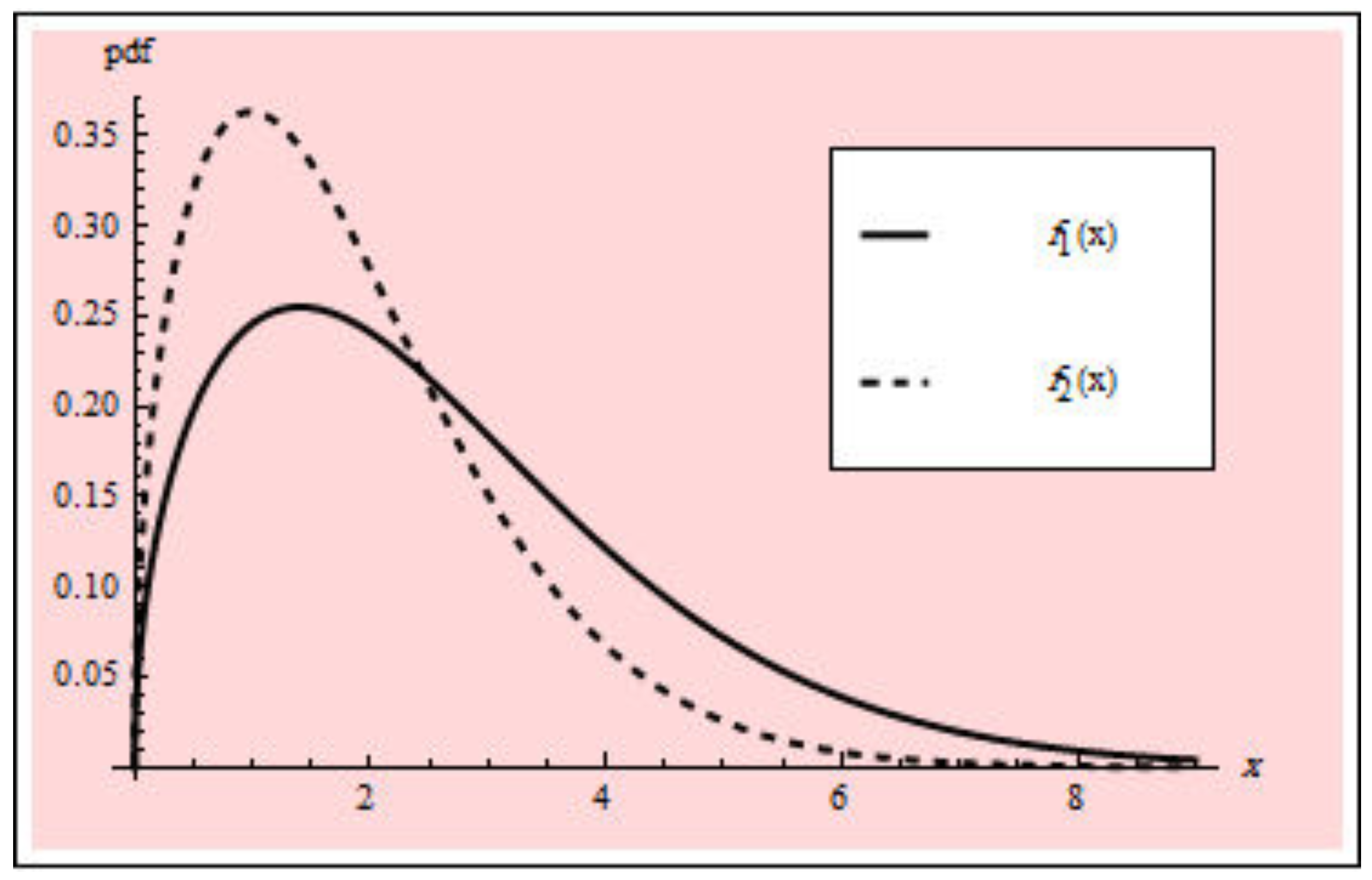
Before moving on, we first determine whether the PHFD can be employed as a suitable model to match the data set using the goodness-of-fit statistic, known as the Kolmogorov–Smirnov (K-S) statistic. The calculated K-S distances and p-values for the data set under the normal and accelerated stress conditions are 0.136924 ( 0.226930 ) and 0.092780 ( 0.700232 ) 
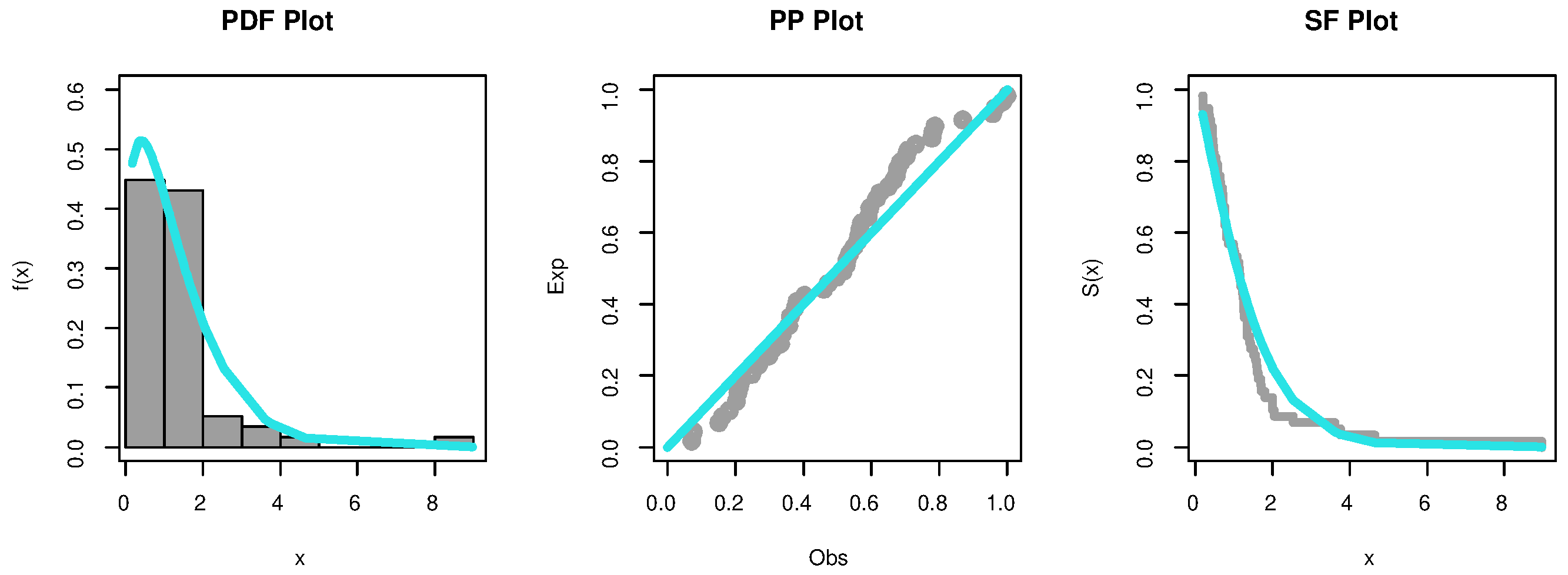
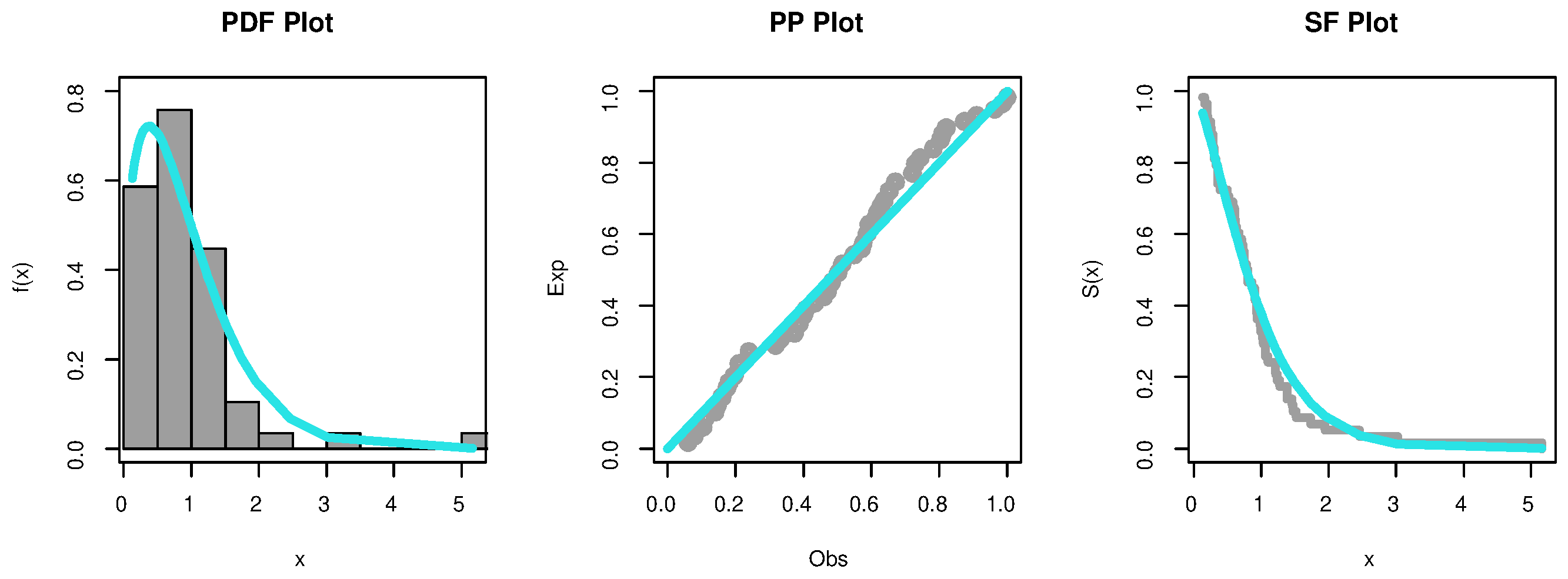
, respectively. The PHFD was found to be a suitable model for this set of data. Further, the empirical PDF, P-P, and SF plots which are shown in Figure 2 and 
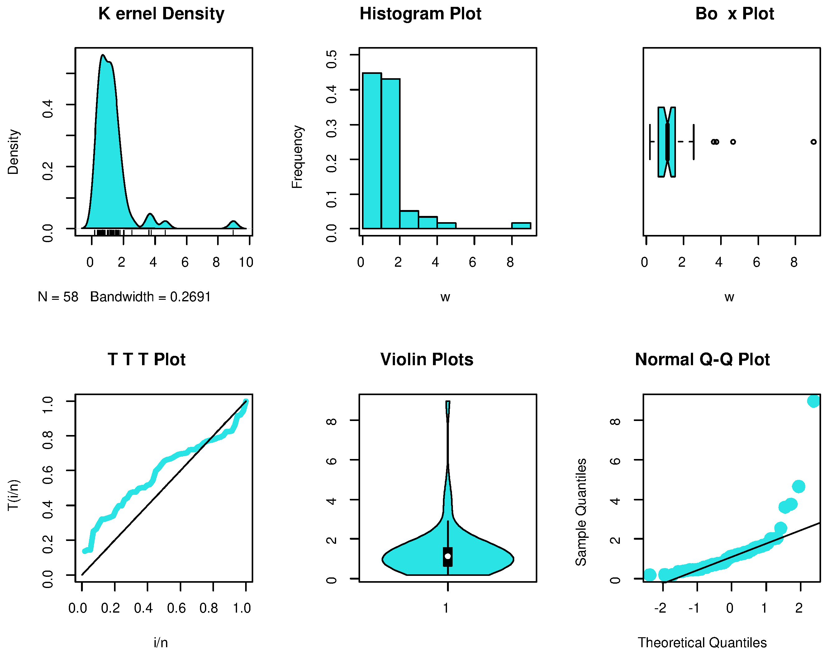
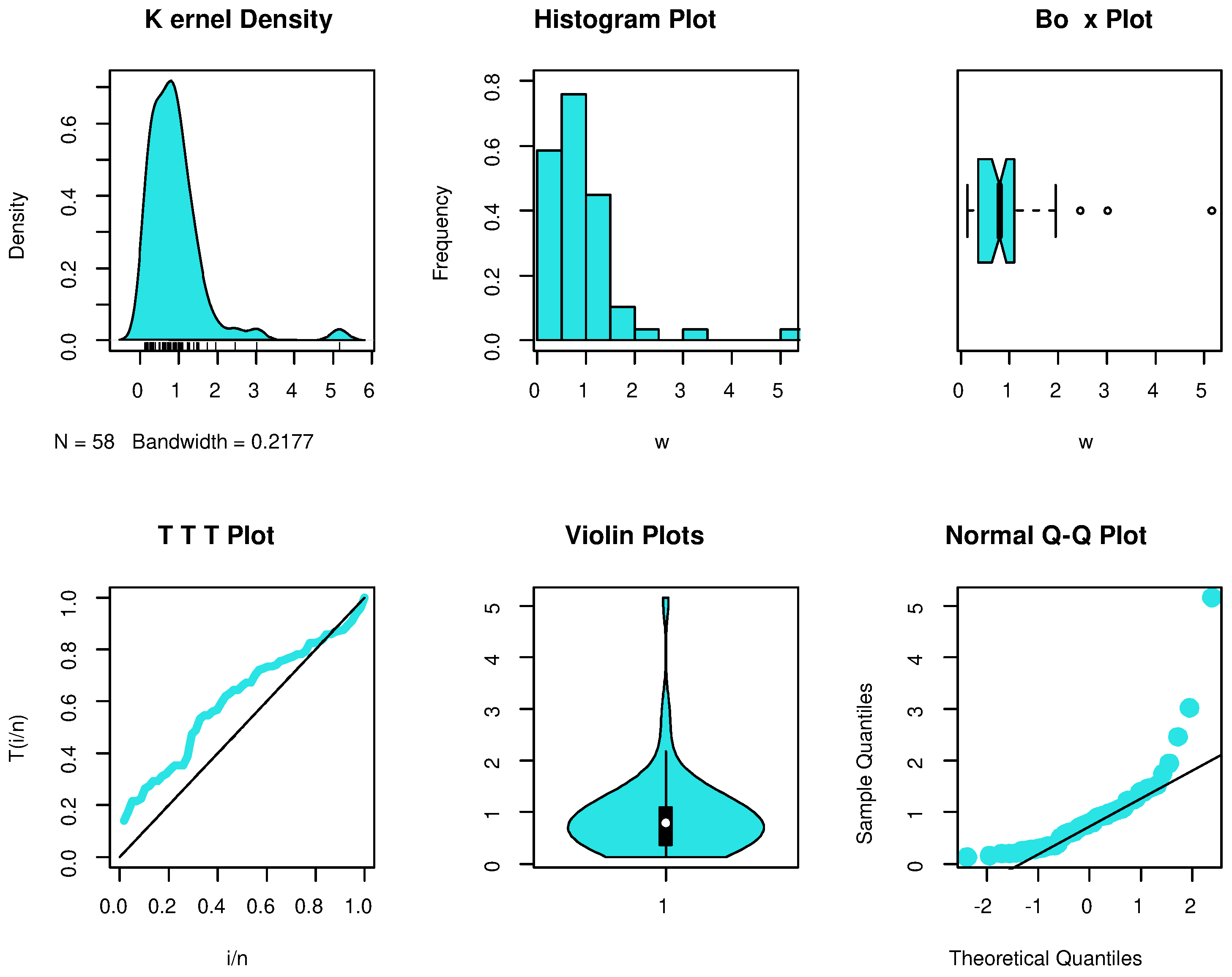
Figure 3 provide additional proof that the PHFD provides a strong fit to the data. Non-parametric approaches, such as histograms, kernel densities, box, violin, TTT, and standard Q-Q plots, are used in Figure 4 and Figure 5 to depict the initial shape. The asymmetry of the data and the validity of some outlier observations should be highlighted.
By implementing the technique outlined in Section 2, PFFC samples are obtained. The original data under both normal use and accelerated stress conditions are separated into groups of a specific size under the use of CSs. Refer to the details presented in Table 6.
The ML and two parametric Bootstrap point estimates as well as the associated ACIs are obtained and listed in Table 7. By moving to Bayes estimates, since no previous knowledge of the unknown population parameters is provided, the non-informative (or vague) gamma priors are adequate in this situation. In this instance, the hyper-parameters are set to zero ( a i = b i = 0 , i = 1 , 2 ) . As previously mentioned, the Gibbs algorithm relies on Metropolis to produce 12,000 MCMC samples using the β ^ M L , δ ^ M L and ρ ^ M L as initial values at the beginning of the algorithm. Additionally, the Bayes estimates are computed and recorded in Table 7. Finally, we can say that the estimated PHFD offers a superb fit for the provided data and that Bayes estimates performs better than MLEs and bootstrap.

8. Conclusions

This paper highlights the statistical inference issue for a system of CS-PALTs under PFFC when the testing products’ lifetimes follow the PHFD. By reducing the amount of time and test units required, and hence the cost, this combination makes our study more useful and applicable in the industrial and technical domains. Several techniques have been developed throughout the study to estimate the relevant parameters, the acceleration factor, and the corresponding confidence intervals. Using the observed FIM, the MLEs are obtained as classical estimation, and the related ACIs are established. Also, two parametric Bootstrap estimates (Boot-p and Boot-t) for the relevant parameters are provided for comparison. Due to the difficulties of obtaining Bayes estimates in closed form, the point and interval estimates for the Bayesian approach are created with the use of the MCMC technique. The effectiveness of the suggested methods is examined by in-depth Monte Carlo simulations. The results clearly show that the Boot-t and Bayes estimates outperform the traditional likelihood and Boot-p estimates in terms of performance and accuracy. In the end, a single collection of actual engineering data is examined for more illustration. The study has shown that the PHFD has offered good flexibility for modeling the life test of the light-emitting diode practically. This study is innovative in that it shows that variable sample sizes k 1 and k 2 can be taken into account in each group when a type-II progressively first failure censored sample is employed. This is completely consistent with real-world examples when conducting life tests. Even though progressively first failure type-II censoring and PHFD have received most of our attention in this study, the same approach can be applied to various distribution and censoring methods. The design of the best censoring schemes, the inference of competing risk models with more failure factors, and the statistical prediction of the subsequent order statistics based on the PALTs from PHFD are just a few of the numerous additional tasks that need to be completed in this area. Finally, we advise adopting the MCMC method based on partially accelerated life testing with the progressive first failure type-II censored on data from life testing, reliability modeling, and medical analysis.

Author Contributions

Conceptualization, A.A.-E.-M. and M.E.-M.; Methodology, M.S.E.; Software, A.A.-E.-M., M.S.E., M.E.-M. and R.M.E.-S.; Validation, R.M.E.-S.; Formal analysis, M.S.E. and R.M.E.-S.; Investigation, A.A.-E.-M.; Resources, M.E.-M. and A.A.-B.; Data curation, M.E.-M. and A.A.-B.; Writing—original draft, A.A.-E.-M. and R.M.E.-S.; Writing—review & editing, M.S.E. All authors have read and agreed to the published version of the manuscript.

Funding

This research was funded by Deanship of Scientific Research, Qassim University, Saudi Arabia.

Data Availability Statement

The data sets are available in the paper.

Acknowledgments

Researchers would like to thank the Deanship of Scientific Research, Qassim University for funding publication of this project.

Conflicts of Interest

The authors declare no conflict of interest.

References

  1. Nelson, W.B. Accelerated Life Testing, Statistical Models, Test Plans and Data Analysis; Wiley: New York, NY, USA, 1990. [Google Scholar]
  2. Lin, C.T.; Hsu, Y.Y.; Lee, S.Y.; Balakrishnan, N. Inference on constant stress accelerated life tests for log-location-scale lifetime distributions with Type-I hybrid censoring. J. Stat. Simul. 2019, 89, 720–749. [Google Scholar] [CrossRef]
  3. Dey, S.; Nassar, M. Generalized inverted exponential distribution under constant stress accelerated life test: Different estimation methods with application. Qual. Reliab. Eng. 2020, 36, 1296–1312. [Google Scholar] [CrossRef]
  4. Nooshin, H. Comparison between constant-stress and step-stress accelerated life tests under a cost constraint for progressive Type I censoring. Seq. Anal. 2021, 40, 17–31. [Google Scholar]
  5. Wang, B. Unbiased estimations for the exponential distribution based on step-stress accelerated life-testing data. Appl. Math. Comput. 2006, 173, 1227–1237. [Google Scholar] [CrossRef]
  6. Abdel-Hamid, A.H.; AL-Hussaini, E.K. Progressive stress accelerated life tests under finite mixture models. Metrika 2007, 66, 213–231. [Google Scholar] [CrossRef]
  7. Kumar, A.; Dey, S.; Tripathi, Y.M. Statistical inference on progressive-stress accelerated lifetesting for the logistic exponential distribution under progressive Type-II censoring. Qual. Reliabil. Eng. Int. 2020, 36, 112–124. [Google Scholar] [CrossRef]
  8. EL-Sagheer, R.M. Inferences in constant-partially accelerated life tests based on progressive type-II censoring. Bull. Malays. Sci. Soc. 2018, 41, 609–626. [Google Scholar] [CrossRef]
  9. Mahmoud, M.A.W.; EL-Sagheer, R.M.; Abou-Senna, A.M. Estimating the modified Weibull parameters in presence of constant-stress partiallyaccelerated life testing. J. Stat. Theory Appl. 2018, 17, 242–260. [Google Scholar] [CrossRef]
  10. Ismail, A. Likelihood inference for a step-stress partially accelerated life test model with type-I progressively hybrid censored data from Weibull distribution. J. Stat. Comput. Simul. 2014, 84, 2486–2494. [Google Scholar] [CrossRef]
  11. Nassar, M.; Farouq, M. Analysis of modified kies exponential distribution with constant stress partially accelerated life tests under type-II censoring. Mathematics 2022, 10, 819. [Google Scholar] [CrossRef]
  12. EL-Sagheer, R.M.; Mahmoud, M.A.W.; Nagaty, H. Inferences for Weibull-exponential distribution based on progressive Type-II censoring under step-stress partially accelerated life test model. J. Stat. Theory Pract. 2019, 13, 13–14. [Google Scholar] [CrossRef]
  13. El-Morshedy, M.; Aljohani, H.M.; Eliwa, M.S.; Nassar, M.; Shakhatreh, M.K.; Afify, A.Z. The exponentiated Burr-Hatke distribution and its discrete version: Reliability properties with CSALT model, inference and applications. Mathematics 2021, 9, 2277. [Google Scholar] [CrossRef]
  14. EL-Sagheer, R.M.; Ahsanullah, M. Statistical inference for a step-stress partially accelerated lifetest model based on progressively type-II censored data from lomax distribution. Appl. Stat. Sci. 2015, 21, 307–323. [Google Scholar]
  15. Sajid, A.; Aslam, M. Choice of suitable informative prior for the scale parameter of mixture of Laplace distribution using Type-I censoring scheme under diffeerent loss function. Electron. J. Appl. Stat. Anal. 2013, 6, 32–56. [Google Scholar]
  16. Ali, A.; Almarashi, A.M.; Okasha, H.; Ng, H.K.T. E-Bayesian estimation of Chen distribution based on Type-I censoring scheme. Entropy 2020, 22, 636. [Google Scholar]
  17. Balakrishnan, N.; Han, D. Exact inference for a simple step-stress model with competing risks for failure from exponential distribution under Type-II censoring. J. Stat. Plan. Inference 2008, 138, 4172–4186. [Google Scholar] [CrossRef]
  18. Balakrishnan, N.; Sandhu, R.A. A simple simulation algorithm for generating progressively type-II censored samples. Am. Stat. 1995, 49, 229–230. [Google Scholar]
  19. Balakrishnan, N. Progressive censoring methodology: An appraisal. Test 2007, 16, 21–259. [Google Scholar] [CrossRef]
  20. EL-Sagheer, R.M. Estimation of parameters of Weibull-Gamma distribution based on progressively censored data. Stat. Pap. 2018, 59, 725–757. [Google Scholar] [CrossRef]
  21. Wu, J.W.; Hung, W.L.; Tsai, C.H. Estimation of the parameters of the Gompertz distribution under the first failure-censored sampling plan. Statistics 2003, 37, 517–525. [Google Scholar] [CrossRef]
  22. Wu, S.J.; Kuş, C. On estimation based on progressive first-failure-censored sampling. Comput. Stat. Data Anal. 2009, 53, 3659–3670. [Google Scholar] [CrossRef]
  23. Saini, S.; Tomer, S.; Garg, R. On the reliability estimation of multicomponent stress-strength model for Burr XII distribution using progressively first-failure censored samples. J. Stat. Comput. Simul. 2022, 92, 667–704. [Google Scholar] [CrossRef]
  24. Ahmadi, M.V.; Doostparast, M. Pareto analysis for the lifetime performance index of products on the basis of progressively first-failure-censored batches under balanced symmetric and asymmetric loss functions. J. Appl. Stat. 2019, 46, 1196–1227. [Google Scholar] [CrossRef]
  25. EL-Sagheer, R.M.; Muqrin, M.A.; El-Morshedy, M.; Eliwa, M.S.; Eissa, F.H.; Abdo, D.A. Bayesian inferential approaches and bootstrap for the reliability and hazard rate functions under progressive first-failure censoring for coronavirus data from asymmetric model. Symmetry 2022, 14, 956. [Google Scholar] [CrossRef]
  26. Prakash, G.; Singh, P. Bound lengths based on constant-stress PALT under different censoring patterns. Int. J. Sci. World 2018, 6, 19–26. [Google Scholar] [CrossRef]
  27. Zhuang, L.; Xu, A.; Wang, X. A prognostic driven predictive maintenance framework based on Bayesian deep learning. Reliab. Eng. Syst. Saf. 2023, 234, 109181. [Google Scholar] [CrossRef]
  28. Luo, C.; Shen, L.; Xu, A. Modelling and estimation of system reliability under dynamic operating environments and lifetime ordering constraints. Reliab. Eng. Syst. Saf. 2022, 218, 108136. [Google Scholar] [CrossRef]
  29. Zhou, S.; Xu, A.; Tang, Y.; Shen, L. Fast Bayesian inference of reparameterized gamma process with random effects. IEEE Trans. Reliab. 2023; in press. [Google Scholar] [CrossRef]
  30. Eliwa, M.S.; Ahmed, E.A. Reliability analysis of constant partially accelerated life tests under progressive first failure type-II censored data from Lomax model: EM and MCMC algorithms. AIMS Math. 2023, 8, 29–60. [Google Scholar] [CrossRef]
  31. Meniconi, B.; Barry, D.M. The power function distribution: A useful and simple distribution to asses’ electrical component reliability. Microelectron. Reliab. 1995, 36, 1207–1212. [Google Scholar] [CrossRef]
  32. Mugdadi, A.R. The least squares type estimation of the parameters in the power hazard function. Appl. Math. Comput. 2005, 169, 737–748. [Google Scholar] [CrossRef]
  33. Mugdadi, A.; Min, A. Bayes estimation of the power hazard function. J. Interdiscip. Math. 2009, 12, 675–689. [Google Scholar] [CrossRef]
  34. Kınacı, I. Estimation of P(Y<X) for distributions having power hazard function. Pak. J. Stat. 2014, 30, 57–70. [Google Scholar]
  35. EL-Sagheer, R.M. Estimation of the parameters of life for distributions having power hazard function based on progressively Type-II censored data. Adv. Appl. Stat. 2015, 45, 1–27. [Google Scholar]
  36. Khan, M.I. The distribution having power hazard function based on orderd random variables. J. Stat. Appl. Probab. Lett. 2017, 4, 33–36. [Google Scholar] [CrossRef]
  37. EL-Sagheer, R.M.; Jawa, T.M.; Sayed, A.N. Assessing the lifetime performance index with digital inferences of power hazard function distribution using progressive type-II censoring scheme. Comput. Intell. Neurosci. 2022, 10, 6467724. [Google Scholar] [CrossRef]
  38. Meeker, W.Q.; Escobar, L.A. Statistical Methods for Reliability Data; Wiley: New York, NY, USA, 1998. [Google Scholar]
  39. Efron, B. The Bootstrap and Other Resampling Plans; Society for Industrial and Applied Mathematics: Philadelphia, PA, USA, 1982. [Google Scholar]
  40. Hall, P. Theoretical comparison of Bootstrap confidence intervals. Ann. Stat. 1988, 16, 927–953. [Google Scholar] [CrossRef]
  41. Arnold, B.C.; Press, S.J. Bayesian inference for Pareto populations. Econometrics 1983, 21, 287–306. [Google Scholar] [CrossRef]
  42. Upadhyay, S.K.; Vasistha, N.; Smith, A.F.M. Bayes inference in life testing and reliability via Markov chain Monte Carlo simulation. Sankhya A 2001, 63, 15–40. [Google Scholar]
  43. Kundu, D.; Howlader, H. Bayesian inference and prediction of the inverse Weibull distribution for Type-II censored data. Comput. Stat. Data Anal. 2010, 54, 1547–1558. [Google Scholar] [CrossRef]
  44. Metropolis, N.A.W.; Rosenbluth, M.N.; Teller, A.H.; Teller, E. Equation of state calculations by fast computing machines. J. Chem. Phys. 1953, 21, 1087–1092. [Google Scholar] [CrossRef]
  45. Tierney, L. Markov chains for exploring posterior distributions (with discussion). Ann. Stat. 1994, 22, 1701–1762. [Google Scholar]
  46. Nassar, M.; Alotaibi, R.; Elshahhat, A. Reliability estimation of XLindley constant-stress partially accelerated life tests using progressively censored samples. Mathematics 2023, 11, 1331. [Google Scholar] [CrossRef]
  47. Dey, S.; Wang, L.; Nassar, M. Inference on Nadarajah-Haghighi distribution with constant stress partially accelerated life tests under progressive Type-II censoring. J. Appl. Stat. 2022, 49, 2891–2912. [Google Scholar] [CrossRef] [PubMed]
  48. Cheng, Y.F.; Wang, F.K. Estimating the Burr XII parameters in constant stress partially accelerated life tests under multiple censored data. Commun.-Stat.-Simul. Comput. 2012, 41, 1711–1727. [Google Scholar] [CrossRef]
Figure 1. PDFs under normal and accelerated conditions.
Mathematics 11 04323 g001
Figure 2. Empirical PDF, P-P, and SF plots for normal condition.
Mathematics 11 04323 g002
Figure 3. Empirical PDF, P-P, and SF plots for accelerated condition.
Mathematics 11 04323 g003
Figure 4. Non-parametric plots for normal condition.
Mathematics 11 04323 g004
Figure 5. Non-parametric plots for accelerated condition.
Mathematics 11 04323 g005
Table 1. MSE of estimates for the parameters β and δ .
β δ
( k , n , m 1 , m 2 ) CS ML Boot-p Boot-t Bayes ML Boot-p Boot-t Bayes
( 2 , 40 , 15 , 15 ) I0.225460.235470.204170.186520.334570.324850.306350.28965
II0.246870.254730.225630.199680.356470.347830.329680.30124
III0.273650.264750.239840.223640.378560.364510.347890.32658
( 2 , 40 , 20 , 25 ) I0.176350.173350.153640.134780.293650.286470.264550.24365
II0.196350.191240.173650.158790.312540.306540.285740.26458
III0.233450.226540.206580.186570.356470.349980.324560.29571
( 2 , 60 , 30 , 30 ) I0.145320.141100.123650.108590.256480.247820.230110.21109
II0.159980.153660.139480.119320.274570.264750.249860.22145
III0.169970.169840.156210.132650.305640.296580.276940.24362
( 2 , 60 , 35 , 40 ) I0.119970.109990.095870.911240.214560.205480.183250.15964
II0.126580.119650.106890.094630.235470.224570.198750.17145
III0.134750.129680.116540.105560.256390.245730.221430.20325
( 2 , 90 , 45 , 45 ) I0.099670.097450.088690.082340.186350.180020.159680.13124
II0.105680.110020.093780.089680.212450.203210.176630.15347
III0.120650.118900.105540.999760.234750.226570.196610.16999
( 2 , 90 , 60 , 75 ) I0.093450.091640.083450.079650.156350.146580.130010.11475
II0.973670.095350.091280.084670.176580.165840.153480.13554
III0.103690.100240.097860.091640.202140.196480.176530.14587
( 4 , 40 , 15 , 15 ) I0.265480.255450.224160.206530.354560.344870.326360.29999
II0.276550.265470.246350.214550.373650.367840.346210.32632
III0.293650.284560.264590.235870.396520.388430.364270.33994
( 4 , 40 , 20 , 25 ) I0.196390.193390.173680.154790.333640.326460.294540.27361
II0.213560.210120.198750.173480.356520.347210.312650.29478
III0.238540.231870.213650.195970.374520.365430.346520.31247
( 4 , 60 , 30 , 30 ) I0.175340.171130.153640.138520.286460.277830.250240.23128
II0.196580.186350.169960.150230.302450.296540.276830.25362
III0.213450.206890.189650.176470.326540.314750.290120.26948
( 4 , 60 , 35 , 40 ) I0.139980.129960.115810.101250.244530.235470.203260.17965
II0.152340.146870.128970.110120.264810.256440.223450.19634
III0.171240.165890.146580.130110.286350.274610.248670.21543
( 4 , 90 , 45 , 45 ) I0.119680.107440.098660.092330.216360.200030.179690.14125
II0.135460.128960.105540.099890.231540.225470.195680.16532
III0.148960.139970.118560.107430.254730.245160.223410.18678
( 4 , 90 , 60 , 75 ) I0.103460.100050.093440.089660.186340.176570.150020.12671
II0.115970.110630.105570.097640.215480.203620.176950.14635
III0.131240.128970.118690.103230.236840.224570.196320.17021
Table 2. MSE of estimates for the parameter ρ .
( k , n , m 1 , m 2 ) CSMLBoot-pBoot-tBayes
( 2 , 40 , 15 , 15 ) I0.526340.516350.476540.42658
II0.536420.523690.496520.45234
III0.564710.556320.523620.47685
( 2 , 40 , 20 , 25 ) I0.496320.486570.423640.39874
II0.512430.502470.456320.41867
III0.536240.524630.475620.43869
( 2 , 60 , 30 , 30 ) I0.457830.445680.387450.35476
II0.476950.463570.406930.37985
III0.498630.486550.436750.40127
( 2 , 60 , 35 , 40 ) I0.412360.402380.359680.32154
II0.436580.425630.374540.34578
III0.461120.450270.403210.36942
( 2 , 90 , 45 , 45 ) I0.376950.365460.312580.28994
II0.395420.384560.341270.31253
III0.412580.403570.371240.34624
( 2 , 90 , 60 , 75 ) I0.336420.321450.286350.24751
II0.356280.346580.305470.27136
III0.375640.364720.334530.29954
( 4 , 40 , 15 , 15 ) I0.546350.536360.496550.44657
II0.562430.553640.512470.47635
III0.586720.574630.532410.49356
( 4 , 40 , 20 , 25 ) I0.516340.506550.443660.42875
II0.536240.524710.465720.44632
III0.563280.554730.486520.46211
( 4 , 60 , 30 , 30 ) I0.477820.465690.407460.37475
II0.493630.486570.428690.39674
III0.513640.504720.453620.42578
( 4 , 60 , 35 , 40 ) I0.432370.422390.379670.34155
II0.453620.445720.394520.36973
III0.489650.476580.425830.39112
( 4 , 90 , 45 , 45 ) I0.396960.385450.332570.30995
II0.412830.403240.362540.32164
III0.446580.436570.396550.36442
( 4 , 90 , 60 , 75 ) I0.356420.341450.306350.26751
II0.376250.370010.324870.28974
III0.412350.405860.356460.31587
Table 3. AWs and CPs of estimates for the parameter β .
( k , n , m 1 , m 2 ) CSMLEBoot-pBoot-tBayes
ACIs ACIs ACIs CRIs
AWs CPs AWs CPs AWs CPs AWs CPs
( 2 , 40 , 15 , 15 ) I3.25360.9413.15620.9512.99740.9512.92650.959
II3.27850.9393.18470.9413.10470.9542.98470.954
III3.32460.9383.23540.9453.16480.9493.10250.951
( 2 , 40 , 20 , 25 ) I3.13460.9413.09940.9432.85750.9472.79960.961
II3.19540.9423.11680.9502.93470.9482.84650.974
III3.22460.9293.16480.9392.98770.9512.93640.963
( 2 , 60 , 30 , 30 ) I3.02580.9382.95780.9542.77540.9502.67890.955
II3.10450.9373.09870.9412.83460.9552.72450.958
III3.15670.9413.10110.9392.91240.9542.86540.963
( 2 , 60 , 35 , 40 ) I2.95670.9382.88360.9382.66480.9492.57630.964
II2.99970.9372.94750.9412.71350.9422.63450.954
III3.12450.9413.08990.9422.83660.9472.75410.971
( 2 , 90 , 45 , 45 ) I2.87460.9432.79860.9472.55640.9512.49750.972
II2.92570.9392.83450.9512.59870.9462.55630.966
III2.97650.9372.88410.9462.66340.9552.59460.967
( 2 , 90 , 60 , 75 ) I2.75680.9512.68990.9422.47570.9532.39990.958
II2.83640.9482.72460.9432.53760.9552.44620.955
III2.88220.9432.78640.9412.59470.9512.51460.957
( 4 , 40 , 15 , 15 ) I3.35360.9523.25620.9513.19740.9493.09260.962
II3.41250.9543.31540.9523.22460.9483.11240.958
III3.48550.9473.36980.9443.29970.9513.19940.962
( 4 , 40 , 20 , 25 ) I3.23470.9463.19930.9372.95760.9532.83950.958
II3.31450.9373.25640.9513.10450.9522.94570.961
III3.37650.9383.31450.9473.22470.9563.10460.962
( 4 , 60 , 30 , 30 ) I3.12540.9413.05790.9392.87570.9572.77860.958
II3.25470.9443.11470.9382.94560.9552.83590.956
III3.32540.9403.21690.9413.14560.9542.92480.955
( 4 , 60 , 35 , 40 ) I3.07660.9512.98370.9362.76490.9532.64620.961
II3.13650.9493.06890.9412.83650.9492.71540.960
III3.23550.9503.13470.9452.94460.9552.81220.958
( 4 , 90 , 45 , 45 ) I2.97450.9292.89850.9432.65650.9482.59760.957
II3.09970.9552.96480.9332.72530.9592.65410.964
III3.16050.9413.07650.9412.82230.9582.74460.955
( 4 , 90 , 60 , 75 ) I2.85670.9492.78980.9512.57580.9542.49950.974
II2.91240.9342.82470.9522.66470.9532.57310.966
III2.99990.9412.89760.9492.77640.9552.64740.962
Table 4. AWs and CPs of estimates for the parameter δ .
( k , n , m 1 , m 2 ) CSMLEBoot-pBoot-tBayes
ACIs ACIs ACIs CRIs
AWs CPs AWs CPs AWs CPs AWs CPs
( 2 , 40 , 15 , 15 ) I2.04560.9391.89470.9411.74580.9411.69780.958
II2.13540.9371.93650.9451.86570.9451.72450.956
III2.36540.9512.05840.9431.96580.9481.86540.955
( 2 , 40 , 20 , 25 ) I1.86540.9481.75480.9501.66450.9461.54710.961
II1.93450.9431.86730.9391.76540.9441.67450.960
III2.13460.9521.96940.9541.85680.9521.75890.958
( 2 , 60 , 30 , 30 ) I1.65470.9541.56940.9411.45730.9511.33650.957
II1.75480.9391.69470.9391.55760.9521.42890.964
III1.83450.9371.77840.9411.65320.9541.53640.955
( 2 , 60 , 35 , 40 ) I1.46980.9511.36870.9451.30010.9511.28740.974
II1.56430.9481.45680.9431.49990.9541.35680.958
III1.66370.9431.55870.9501.50030.9491.43460.956
( 2 , 90 , 45 , 45 ) I1.26540.9521.15470.9391.11360.9471.09960.955
II1.36540.9541.27560.9541.21360.9481.15640.961
III1.45870.9391.36540.9411.31220.9511.24560.960
( 2 , 90 , 60 , 75 ) I1.17690.9371.09870.9391.07780.9501.06580.958
II1.23650.9511.16470.9411.10340.9551.10010.957
III1.31240.9481.25460.9451.18650.9541.12360.964
( 4 , 40 , 15 , 15 ) I2.14540.9431.99480.9431.84570.9511.79790.955
II2.23650.9522.14570.9501.96580.9541.85470.974
III2.36910.9542.25740.9392.13650.9491.94320.958
( 4 , 40 , 20 , 25 ) I1.96550.9391.85490.9541.76440.9471.64720.956
II2.05470.9371.93580.9411.85760.9481.75690.955
III2.13690.9512.09650.9391.96580.9511.86940.961
( 4 , 60 , 30 , 30 ) I1.75480.9481.66950.9411.55740.9501.43660.960
II1.84760.9431.77640.9451.65470.9551.54670.958
III1.95680.9521.86490.9431.74660.9541.65730.957
( 4 , 60 , 35 , 40 ) I1.56970.9541.46860.9501.40020.9511.38750.964
II1.66940.9411.54730.9391.50120.9541.47680.955
III1.75890.9391.63770.9541.59990.9491.51520.974
( 4 , 90 , 45 , 45 ) I1.36520.9371.25480.9411.21370.9471.15930.961
II1.45860.9511.34750.9391.31040.9481.24680.960
III1.56240.9481.45860.9291.40070.9511.35670.959
( 4 , 90 , 60 , 75 ) I1.27670.9431.19880.9411.15760.9501.10510.953
II1.36540.9521.26890.9391.21450.9551.16980.961
III1.46520.9541.35840.9411.29970.9541.25630.959
Table 5. AWs and CPs of estimates for the parameter ρ .
( k , n , m 1 , m 2 ) CSMLEBoot-pBoot-tBayes
ACIs ACIs ACIs CRIs
AWs CPs AWs CPs AWs CPs AWs CPs
( 2 , 40 , 15 , 15 ) I4.05640.9293.86540.9393.65480.9472.95840.951
II4.26580.9554.05690.9543.86140.9483.16530.958
III4.46350.9414.23550.9414.05630.9513.46580.957
( 2 , 40 , 20 , 25 ) I3.73650.9493.54680.9393.36590.9503.01250.964
II3.96520.9343.76590.9413.54760.9553.24860.955
III4.13650.9293.92540.9393.74630.9543.31920.974
( 2 , 60 , 30 , 30 ) I3.55640.9553.36840.9543.14680.9472.85670.958
II3.76850.9413.54770.9413.36980.9483.05680.957
III3.94760.9493.76660.9393.55740.9513.26950.964
( 2 , 60 , 35 , 40 ) I3.36590.9343.14570.9412.87450.9502.65470.955
II3.56870.9293.33940.9393.16920.9552.79540.974
III3.69850.9553.51470.9543.29980.9543.00450.958
( 2 , 90 , 45 , 45 ) I3.12540.9412.79940.9412.59980.9472.45770.957
II3.32580.9492.99570.9392.79840.9482.59690.964
III3.54620.9343.25980.9413.02430.9512.86350.955
( 2 , 90 , 60 , 75 ) I2.99650.9292.69540.9392.38740.9502.24660.974
II3.15640.9552.85470.9542.51460.9552.37210.958
III3.34670.9413.01190.9412.75680.9542.55990.957
( 4 , 40 , 15 , 15 ) I4.25640.9494.06540.9393.85480.9473.15840.964
II4.46890.9344.26580.9414.06540.9483.25810.955
III4.59560.9294.43650.9394.19970.9513.58760.974
( 4 , 40 , 20 , 25 ) I3.93650.9553.74680.9543.56590.9503.21250.958
II4.13580.9413.95240.9413.74560.9553.46580.957
III4.36920.9494.13650.9393.96470.9543.65240.964
( 4 , 60 , 30 , 30 ) I3.75630.9343.56850.9413.24670.9473.05680.955
II3.96580.9293.74580.9393.45780.9483.19950.974
III4.15680.9553.96510.9543.66540.9513.45540.958
( 4 , 60 , 35 , 40 ) I3.56570.9413.34540.9413.07460.9502.85480.957
II3.74410.9493.56620.9393.23130.9553.05330.964
III3.89540.9343.74410.9413.42250.9543.18990.955
( 4 , 90 , 45 , 45 ) I3.32560.9292.98950.9392.79990.9472.65780.974
II3.49960.9553.16450.9542.89740.9482.85570.958
III3.71540.9413.45710.9413.18240.9513.00790.957
( 4 , 90 , 60 , 75 ) I3.10630.9492.89560.9392.58750.9502.44670.964
II3.36510.9383.15870.9432.74580.9552.65520.955
III3.49850.3973.33340.9422.89650.9542.83240.974
Table 6. PFFC under CS-PALT LED failure data.
Normal use condition: ( k 1 , n 1 , m 1 ) = ( 2 , 29 , 15 ) .
R 1 = (3, 1, 1, 2, 0, 1, 2, 1, 0, 2, 0, 1, 0, 0, 0).
0.18, 0.19, 0.36, 0.45, 0.47, 0.57, 0.63, 0.70, 0.71, 0.76, 0.79, 0.85, 1.01, 3.76, 8.97.
Accelerated stress condition: ( k 2 , n 2 , m 2 ) = ( 2 , 29 , 18 ) .
R 2 = (1, 1, 2, 0, 1, 0, 2, 0, 2, 0, 2, 0, 0, 1, 0, 0, 0, 0).
0.13, 0.20, 0.21, 0.26, 0.31, 0.35, 0.50, 0.58, 0.60, 0.63, 0.75, 0.78, 0.80, 0.94, 1.22, 1.95,
2.46, 3.02.
Table 7. Estimates of β , δ , ρ and its corresponding 95 % CI using PFFC under CS-PALT.
Parameter ( . ) ML ( . ) Boot p ( . ) Boot t ( . ) BS
β Estimate1.709851.748651.664731.54899
95 % CI(0.8371, 3.4926)(0.9436, 3.3772)(0.8945, 2.9246)(0.9932, 2.6745)
δ Estimate0.153230.162250.134820.12557
95 % CI(0.0295, 0.7953)(0.0365, 0.8766)(0.0334, 0.7452)(0.0215, 0.6935)
ρ Estimate0.282090.269420.216410.19984
95 % CI(0.1701, 0.4679)(0.1432, 0.5211)(0.1165, 0.4263)(0.0989, 0.3762)
Disclaimer/Publisher’s Note: The statements, opinions and data contained in all publications are solely those of the individual author(s) and contributor(s) and not of MDPI and/or the editor(s). MDPI and/or the editor(s) disclaim responsibility for any injury to people or property resulting from any ideas, methods, instructions or products referred to in the content.

