
Prediction of Infectious Disease to Reduce the Computation Stress on Medical and Health Care Facilitators

Abstract
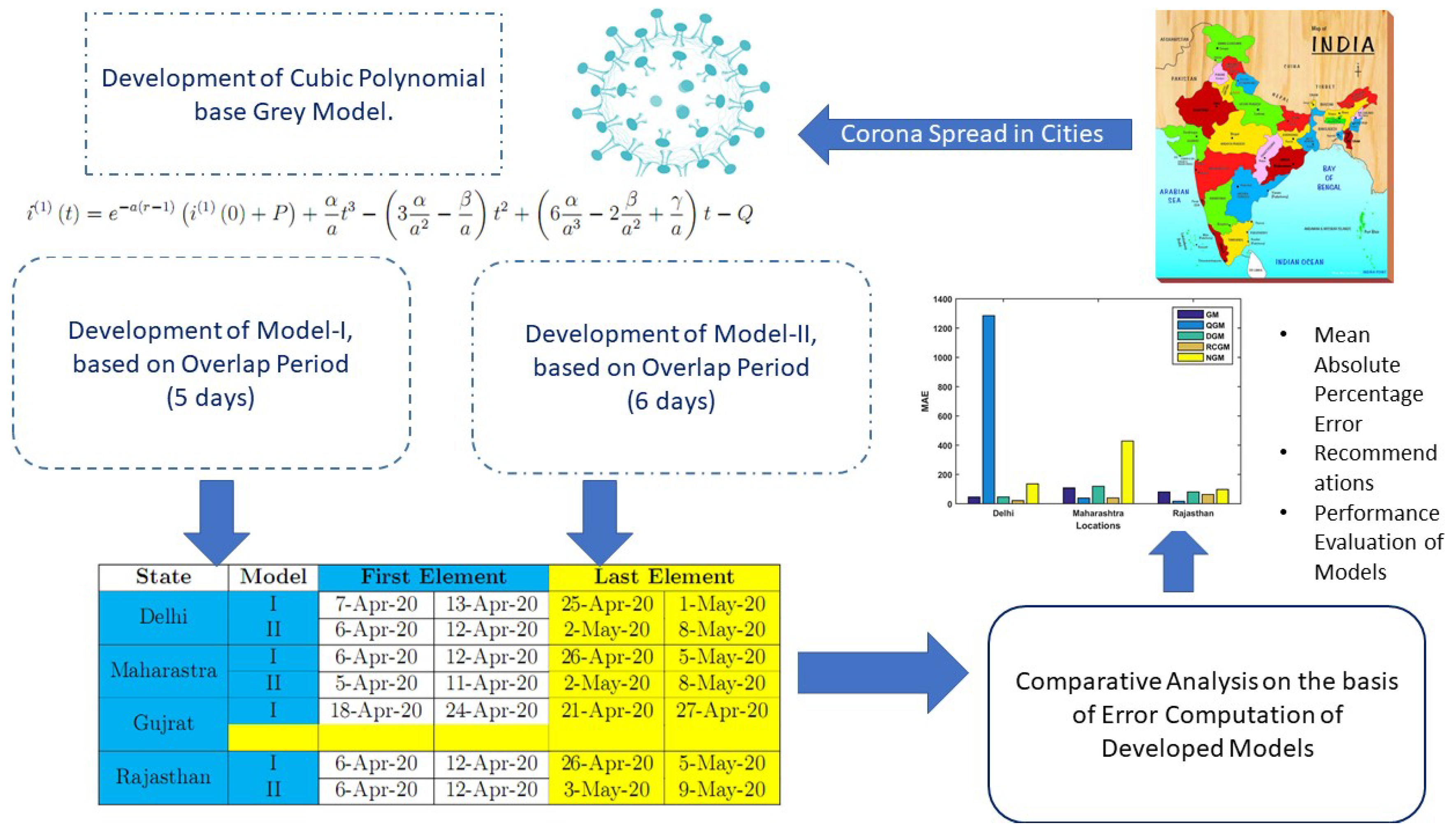
:1. Introduction
- Change in accumulation operator
- Change in back ground value information
- Transformation of the series into a new one in order to deal with negative data.
- 1.
- To develop a rolling horizon based grey model for identification of Novel Corona virus cases in a span of week.
- 2.
- To establish mathematical framework of Cubic polynomial driven grey model by analysing the response and mathematical induction.
- 3.
- To present a comparative analysis of developed models with some known grey models and evaluate the performance with the calculation of various error indices.
- 4.
- To frame the recommendations on the basis of forecasting results for authorities to take preventive steps for combating Corona effectively.
Paper Structure
2. Development of Rolling Horizon Grey Model Comprises with Cubic Polynomial (RCGM)
2.1. Details of Conventional Grey Models
- 1.
- GM(1,1) model: The classical GM(1,1) model is also known as the basic foundation model of grey theory and widely used in the forecasting of data with uncertainty. This model comprises of differential equation varying with time for variance of parameters. The basic equation of this model isThe sequence based on time series is given by
- 2.
- 3.
- NGM(1,1) model: The grey differential equation of NGM [25] isThe time response equation is given byand the restored value is given mathematically as
- 4.
- QGM model: This nonlinear grey model was first proposed by [20] and provide higher prediction accuracy than previously proposed model. The whitenization differential equation of QGM model is represented byThe time response term and restored values can be given as
2.2. Rolling Horizon Based Cubic Grey Model (RCGM)
- Mean Absolute Percentage Error
- Absolute Percentage Error
- Mean Absolute Error
- Mean Square Error
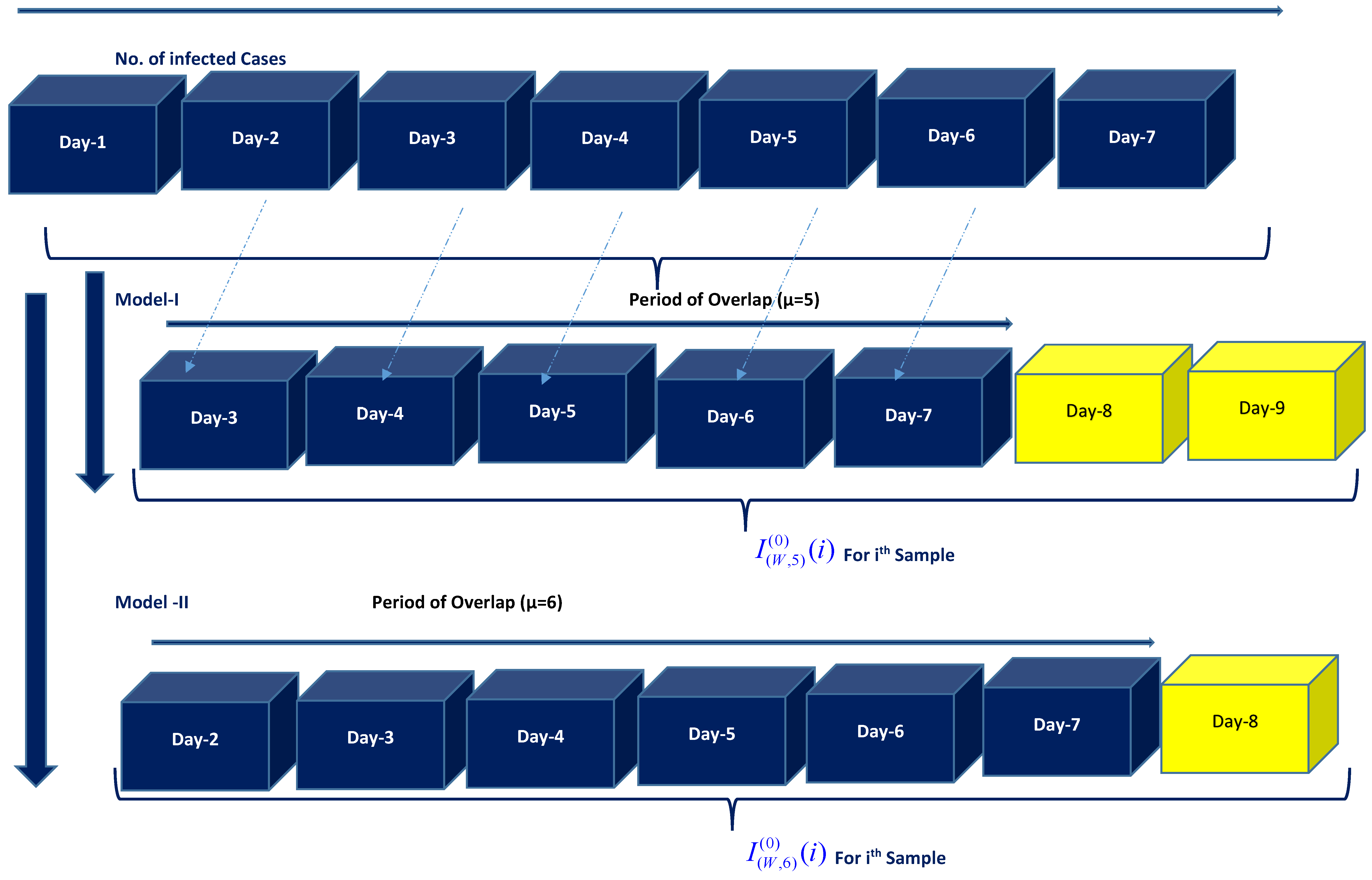
2.3. Development of Rolling Cubic Grey Model (RCGM)
2.4. Discussion
3. Results
3.1. Model I
- 1.
- For obtaining the results of Model-I, the time series is constructed with overlap period of five days and a rolling model is developed by rolling the mean values of a week by two days. The prediction of this series is evaluated with proposed RCGM and four other models such as (GM [23], NGM [24], DGM [38] and QGM [20]).
- 2.
- The prediction results of the states of Maharashtra, Rajasthan and Delhi are shown in tables. These prediction results show that pandemic spread is exponentially increasing in these locations and an acute requirement or advisory is necessary along with the medical help.
- 3.
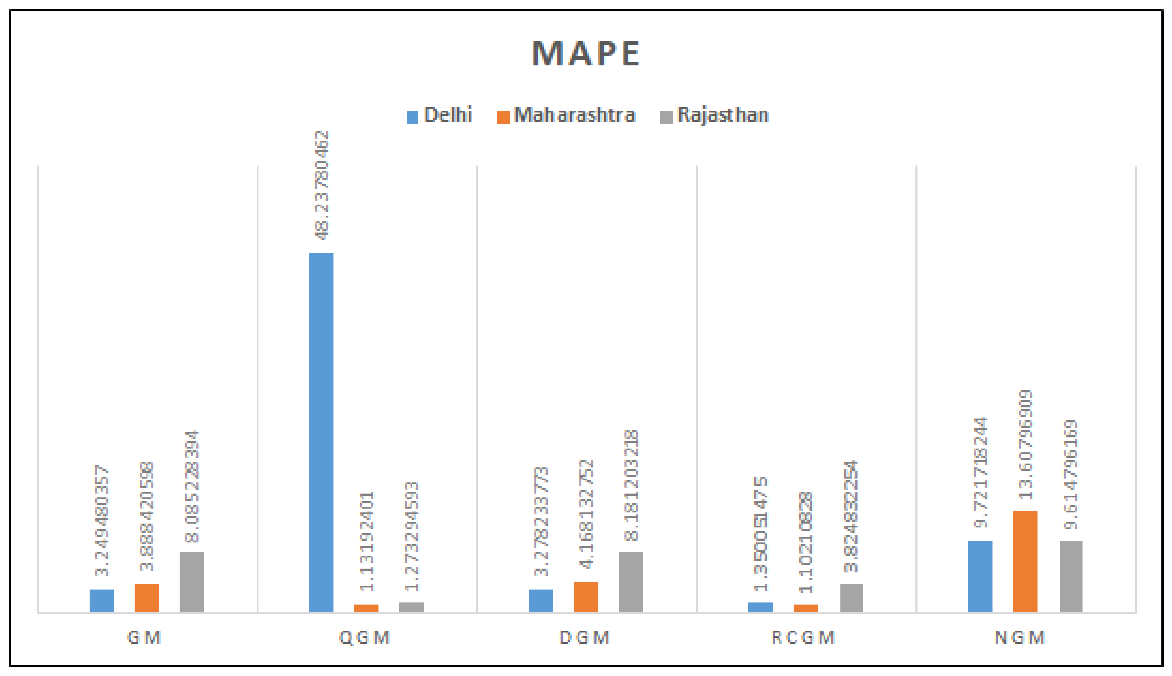
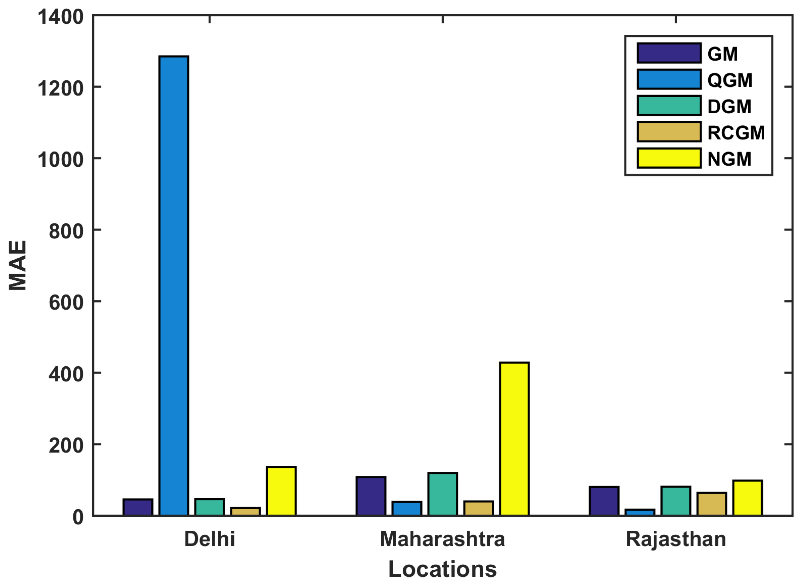
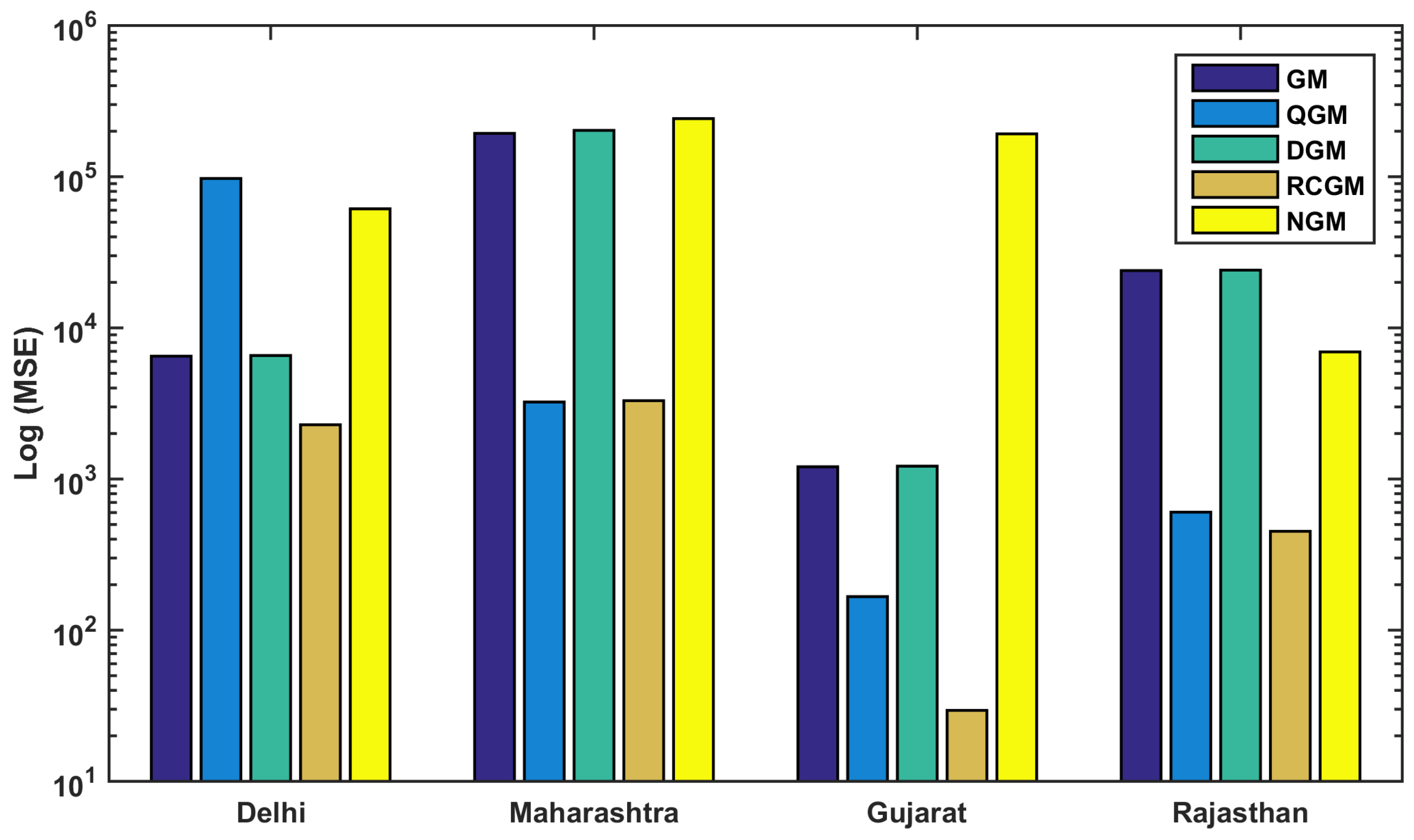
- Inspecting the results of Delhi, we observed that the values of infected cases in the Capital is accurately predicted by RCGM as the value of MAPE is optimal as compared to others. Also, it is observed that the values of MAPE are optimal for state of Maharashtra and Rajasthan. The analysis of the MAPE values are depicted in Figure 3. Addition to that analysis MAE is for these places are also depicted in Figure 4.
3.2. Model II
- 1.
- For obtaining the results of Model-II, the time series is constructed with overlap period of six days and a rolling model is developed again. The prediction of this series is evaluated with proposed RCGM and four other grey models.
- 2.
- The prediction results in terms of MAPE are depicted through Figure 5, from the figure, it is empirical to state that the MAPE values are optimal for proposed model. This fact affirms the applicability of of this RCGM model.
- 3.
- In case of all states along with Delhi, the values of MAPE are optimal. Addition to that, Mean absolute errors are also calculated for this model. Inspecting these values, it is concluded that these values are also quite optimal for RCGM. The analysis of MAE and MSE are shown in Figure 4 and Figure 5.
3.3. Discussion
3.4. Recommendations
- It is empirical to state that the no. of infected cases can be increased in due course of time, hence an acute arrangement of medical facilities and health care related facilities can be appended.
- An awareness program can be initiated for imparting the education to the rural areas about the disease and its implications. Addition to that, an online alert can be issued to major spots and guidelines for travel and other social gatherings can be changed according to the situation.
- Adequate arrangements can be done for converting the unused buildings/schools and colleges for conversion in major relief centres of the corona. Also, the awareness programs can be arranged by the people who have successfully defeated this disease. This can be broadcast on social media and local channels of televisions and radio.
4. Conclusions
- Two time series models based on diverse overlapping periods and rolling horizon are presented. Mathematical representation of these models is presented. Further, the analysis of these models is conducted with the help of COVID-19 case studies at different states of India.
- It has been observed that proposed models produce accurate results as compared to previous reported approaches on the same data. Comparison of the performance of the models has been done on the basis of different error indices evaluation. Further, we argue that due to lack of abundant data, we employ grey model with rolling horizon and also analyses are conducted with the calculation of many indices.
- It is concluded that the proposed approach is effective and yields accurate results and further can be implemented for improving medical facilities and other life supporting resources.
Author Contributions
Funding
Data Availability Statement
Acknowledgments
Conflicts of Interest
References
- Huang, C.; Wang, Y.; Li, X.; Ren, L.; Zhao, J.; Hu, Y.; Zhang, L.; Fan, G.; Xu, J.; Gu, X.; et al. Clinical features of patients infected with 2019 novel coronavirus in Wuhan, China. Lancet 2020, 395, 497–506. [Google Scholar] [CrossRef] [PubMed] [Green Version]
- Vellingiri, B.; Jayaramayya, K.; Iyer, M.; Narayanasamy, A.; Govindasamy, V.; Giridharan, B.; Ganesan, S.; Venugopal, A.; Venkatesan, D.; Ganesan, H.; et al. COVID-19: A promising cure for the global panic. Sci. Total. Environ. 2020, 725, 138277. [Google Scholar] [CrossRef] [PubMed]
- Cucinotta, D.; Vanelli, M. WHO declares COVID-19 a pandemic. Acta Bio Medica Atenei Parm. 2020, 91, 157. [Google Scholar]
- Tobías, A. Evaluation of the lockdowns for the SARS-CoV-2 epidemic in Italy and Spain after one month follow up. Sci. Total. Environ. 2020, 725, 138539. [Google Scholar] [CrossRef] [PubMed]
- Wang, L.; Li, J.; Guo, S.; Xie, N.; Yao, L.; Cao, Y.; Day, S.W.; Howard, S.C.; Graff, J.C.; Gu, T.; et al. Real-time estimation and prediction of mortality caused by COVID-19 with patient information based algorithm. Sci. Total. Environ. 2020, 727, 138394. [Google Scholar] [CrossRef]
- Bräuning, F.; Koopman, S.J. Forecasting macroeconomic variables using collapsed dynamic factor analysis. Int. J. Forecast. 2014, 30, 572–584. [Google Scholar] [CrossRef] [Green Version]
- Wu, L.; Liu, S.; Chen, D.; Yao, L.; Cui, W. Using gray model with fractional order accumulation to predict gas emission. Nat. Hazards 2014, 71, 2231–2236. [Google Scholar] [CrossRef]
- Zhou, W.; He, J.M. Generalized GM (1, 1) model and its application in forecasting of fuel production. Appl. Math. Model. 2013, 37, 6234–6243. [Google Scholar] [CrossRef]
- Zeng, B.; Tan, Y.; Xu, H.; Quan, J.; Wang, L.; Zhou, X. Forecasting the Electricity Consumption of Commercial Sector in Hong Kong Using a Novel Grey Dynamic Prediction Model. J. Grey Syst. 2018, 30, 159–174. [Google Scholar]
- Zhang, Y.; Xu, Y.; Wang, Z. GM (1, 1) grey prediction of Lorenz chaotic system. Chaos Solitons Fractals 2009, 42, 1003–1009. [Google Scholar] [CrossRef]
- Ou, S.L. Forecasting agricultural output with an improved grey forecasting model based on the genetic algorithm. Comput. Electron. Agric. 2012, 85, 33–39. [Google Scholar] [CrossRef]
- Javed, S.A.; Liu, S. Predicting the research output/growth of selected countries: Application of Even GM (1, 1) and NDGM models. Scientometrics 2018, 115, 395–413. [Google Scholar] [CrossRef]
- Lin, W.M.; Hong, C.M.; Huang, C.H.; Ou, T.C. Hybrid control of a wind induction generator based on Grey–Elman neural network. IEEE Trans. Control Syst. Technol. 2013, 21, 2367–2373. [Google Scholar] [CrossRef]
- Xia, M.; Wong, W.K. A seasonal discrete grey forecasting model for fashion retailing. Knowl. Based Syst. 2014, 57, 119–126. [Google Scholar] [CrossRef]
- Chimmula, V.K.R.; Zhang, L. Time series forecasting of COVID-19 transmission in Canada using LSTM networks. Chaos Solitons Fractals 2020, 135, 109864. [Google Scholar] [CrossRef]
- Sahai, A.K.; Rath, N.; Sood, V.; Singh, M.P. ARIMA modelling & forecasting of COVID-19 in top five affected countries. Diabetes Metab. Syndr. Clin. Res. Rev. 2020, 14, 1419–1427. [Google Scholar]
- Rahimi, I.; Chen, F.; Gandomi, A.H. A review on COVID-19 forecasting models. Neural Comput. Appl. 2021, 1–11. [Google Scholar] [CrossRef]
- Ju-Long, D. Control problems of grey systems. Syst. Control Lett. 1982, 1, 288–294. [Google Scholar] [CrossRef]
- Bilgil, H. New grey forecasting model with its application and computer code. AIMS Math. 2021, 6, 1497–1514. [Google Scholar] [CrossRef]
- Zhang, J.; Jiang, Z. A new grey quadratic polynomial model and its application in the COVID-19 in China. Sci. Rep. 2021, 11, 12588. [Google Scholar] [CrossRef]
- Saxena, A. Grey forecasting models based on internal optimization for Novel Corona virus (COVID-19). Appl. Soft Comput. 2021, 111, 107735. [Google Scholar] [CrossRef] [PubMed]
- Ceylan, Z. Short-term prediction of COVID-19 spread using grey rolling model optimized by particle swarm optimization. Appl. Soft Comput. 2021, 109, 107592. [Google Scholar] [CrossRef] [PubMed]
- Akay, D.; Atak, M. Grey prediction with rolling mechanism for electricity demand forecasting of Turkey. Energy 2007, 32, 1670–1675. [Google Scholar] [CrossRef]
- Cui, J.; Liu, S.f.; Zeng, B.; Xie, N.M. A novel grey forecasting model and its optimization. Appl. Math. Model. 2013, 37, 4399–4406. [Google Scholar] [CrossRef]
- Chen, P.Y.; Yu, H.M. Foundation settlement prediction based on a novel NGM model. Math. Probl. Eng. 2014, 2014, 242809. [Google Scholar] [CrossRef] [Green Version]
- Ma, X.; Hu, Y.s.; Liu, Z.b. A novel kernel regularized nonhomogeneous grey model and its applications. Commun. Nonlinear Sci. Numer. Simul. 2017, 48, 51–62. [Google Scholar] [CrossRef]
- Xie, N.m.; Liu, S.f. Discrete grey forecasting model and its optimization. Appl. Math. Model. 2009, 33, 1173–1186. [Google Scholar] [CrossRef]
- Xie, N.M.; Liu, S.F.; Yang, Y.J.; Yuan, C.Q. On novel grey forecasting model based on non-homogeneous index sequence. Appl. Math. Model. 2013, 37, 5059–5068. [Google Scholar] [CrossRef]
- Zeng, B.; Luo, C.; Liu, S.; Li, C. A novel multi-variable grey forecasting model and its application in forecasting the amount of motor vehicles in Beijing. Comput. Ind. Eng. 2016, 101, 479–489. [Google Scholar] [CrossRef]
- Ma, X.; Liu, Z.B. The kernel-based nonlinear multivariate grey model. Appl. Math. Model. 2018, 56, 217–238. [Google Scholar] [CrossRef]
- Zeng, B.; Li, C. Improved multi-variable grey forecasting model with a dynamic background-value coefficient and its application. Comput. Ind. Eng. 2018, 118, 278–290. [Google Scholar] [CrossRef]
- Saxena, A.; Alrasheedi, A.F.; Alnowibet, K.A.; Alshamrani, A.M.; Shekhawat, S.; Mohamed, A.W. Local Grey Predictor Based on Cubic Polynomial Realization for Market Clearing Price Prediction. Axioms 2022, 11, 627. [Google Scholar] [CrossRef]
- Saxena, A. Optimized Fractional Overhead Power Term Polynomial Grey Model (OFOPGM) for market clearing price prediction. Electr. Power Syst. Res. 2023, 214, 108800. [Google Scholar] [CrossRef]
- Saini, V.K.; Kumar, R.; Mathur, A.; Saxena, A. Short term forecasting based on hourly wind speed data using deep learning algorithms. In Proceedings of the 2020 3rd International Conference on Emerging Technologies in Computer Engineering: Machine Learning and Internet of Things (ICETCE), Jaipur, India, 7–8 February 2020; pp. 1–6. [Google Scholar]
- Faghih Mohammadi Jalali, M.; Heidari, H. Predicting changes in Bitcoin price using grey system theory. Financ. Innov. 2020, 6, 13. [Google Scholar] [CrossRef] [Green Version]
- Jiang, P.; Zhou, Q.; Jiang, H.; Dong, Y. An optimized forecasting approach based on grey theory and Cuckoo search algorithm: A case study for electricity consumption in New South Wales. In Abstract and Applied Analysis; Hindawi: London, UK, 2014; Volume 2014, p. 183095. [Google Scholar]
- Zhang, P.; Ma, X.; She, K. A novel power-driven grey model with whale optimization algorithm and its application in forecasting the residential energy consumption in China. Complexity 2019, 2019, 1510257. [Google Scholar] [CrossRef]
- Xie, N.; Liu, S. Discrete GM (1, 1) and mechanism of grey forecasting model. Syst. Eng. Theory Pract. 2005, 1, 93–99. [Google Scholar]
- Ministry of Health and Family Welfare MHFQ COVID-19 India Dataset. 2020. Available online: https://www.mohfw.gov.in/ (accessed on 25 July 2021).
- Kaggle Data. COVID-19 Corona Virus India Dataset. 2020. Available online: https://www.kaggle.com/imdevskp/covid19-corona-virus-india-dataset (accessed on 25 July 2021).


| State | Model | First Element | Last Element | ||
|---|---|---|---|---|---|
| Delhi | I | 7-April-20 | 13-April-20 | 25-April-20 | 1-May-20 |
| II | 6-April-20 | 12-April-20 | 2-May-20 | 8-May-20 | |
| Maharastra | I | 6-April-20 | 12-April-20 | 26-April-20 | 5-May-20 |
| II | 5-April-20 | 11-April-20 | 2-May-20 | 8-May-20 | |
| Gujrat | - | - | - | - | |
| II | 18-April-20 | 24-April-20 | 21-April-20 | 27-April-20 | |
| Rajasthan | I | 6-April-20 | 12-April-20 | 26-April-20 | 5-May-20 |
| II | 6-April-20 | 12-April-20 | 3-May-20 | 9-May-20 | |
| Index | Initial Value | GM | NGM | DGM | QGM | RCGM |
|---|---|---|---|---|---|---|
| 1 | 355.5714 | 355.5714 | 355.5714 | 355.5714 | 355.5714 | 355.5714 |
| 2 | 503.8571 | 694.262 | 332.871 | 697.5088 | 491.9806 | 497.5609 |
| 3 | 685 | 799.4657 | 553.1245 | 803.0879 | 686.1868 | 661.824 |
| 4 | 871.8571 | 920.6112 | 770.0057 | 924.6481 | 883.4866 | 841.5746 |
| 5 | 1061.429 | 1060.114 | 983.5661 | 1064.608 | 1083.353 | 1034.188 |
| 6 | 1256.143 | 1220.757 | 1193.857 | 1225.754 | 1285.349 | 1235.844 |
| 7 | 1493.714 | 1405.742 | 1400.927 | 1411.291 | 1489.112 | 1440.973 |
| 8 | 1727.714 | 1618.758 | 1604.827 | 1624.913 | 1694.341 | 1641.468 |
| 9 | 1933.286 | 1864.053 | 1805.605 | 1870.87 | 1900.786 | 1825.52 |
| 10 | 2111.714 | 2146.519 | 2003.309 | 2154.056 | 2108.24 | 1975.927 |
| 11 | 2278.571 | 2471.788 | 2197.985 | 2480.107 | 2316.531 | 2067.639 |
| Index | Initial Value | GM | NGM | DGM | QGM | RCGM |
|---|---|---|---|---|---|---|
| 1 | 1028.143 | 1028.143 | 1028.143 | 1028.143 | 1028.143 | 1028.143 |
| 2 | 1386.429 | 1662.276 | 778.5358 | 1669.154 | 1424.073 | 1371.877 |
| 3 | 1834.714 | 2006.884 | 1309.287 | 2016.133 | 1806.895 | 1796.358 |
| 4 | 2352.571 | 2422.934 | 1893.203 | 2435.242 | 2285.809 | 2273.47 |
| 5 | 2872.429 | 2925.236 | 2535.608 | 2941.473 | 2865.265 | 2837.874 |
| 6 | 3522.429 | 3531.67 | 3242.362 | 3552.939 | 3549.919 | 3509.077 |
| 7 | 4274.857 | 4263.826 | 4019.911 | 4291.514 | 4344.643 | 4298.055 |
| 8 | 5234.714 | 5147.765 | 4875.345 | 5183.623 | 5254.533 | 5210.985 |
| 9 | 6355 | 6214.956 | 5816.466 | 6261.181 | 6284.923 | 6251.342 |
| 10 | 7500.429 | 7503.386 | 6851.859 | 7562.738 | 7441.394 | 7421.084 |
| 11 | 8690.571 | 9058.924 | 7990.964 | 9134.86 | 8729.784 | 8721.31 |
| Index | Initial value | GM | NGM | DGM | QGM | RCGM |
|---|---|---|---|---|---|---|
| 1 | 355.5714 | 355.5714 | 355.5714 | 355.5714 | 355.5714 | 355.5714 |
| 2 | 503.8571 | 694.262 | 332.871 | 697.5088 | 491.9806 | 497.5609 |
| 3 | 685 | 799.4657 | 553.1245 | 803.0879 | 686.1868 | 661.824 |
| 4 | 871.8571 | 920.6112 | 770.0057 | 924.6481 | 883.4866 | 841.5746 |
| 5 | 1061.429 | 1060.114 | 983.5661 | 1064.608 | 1083.353 | 1034.188 |
| 6 | 1256.143 | 1220.757 | 1193.857 | 1225.754 | 1285.349 | 1235.844 |
| 7 | 1493.714 | 1405.742 | 1400.927 | 1411.291 | 1489.112 | 1440.973 |
| 8 | 1727.714 | 1618.758 | 1604.827 | 1624.913 | 1694.341 | 1641.468 |
| 9 | 1933.286 | 1864.053 | 1805.605 | 1870.87 | 1900.786 | 1825.52 |
| 10 | 2111.714 | 2146.519 | 2003.309 | 2154.056 | 2108.24 | 1975.927 |
| 11 | 2278.571 | 2471.788 | 2197.985 | 2480.107 | 2316.531 | 2067.639 |
| Index | Initial Value | GM | NGM | DGM | QGM | RCGM |
|---|---|---|---|---|---|---|
| 1 | 664 | 664 | 664 | 664 | 664 | 664 |
| 2 | 744.8571 | 974.7736 | 236.7698 | 975.3504 | 800.5598 | 757.1481 |
| 3 | 835 | 1036.207 | 395.2235 | 1036.827 | 905.0348 | 903.6271 |
| 4 | 968.4286 | 1101.511 | 553.189 | 1102.179 | 1010.093 | 1039.558 |
| 5 | 1109.143 | 1170.932 | 710.6676 | 1171.65 | 1115.872 | 1166.29 |
| 6 | 1239 | 1244.727 | 867.661 | 1245.5 | 1222.545 | 1285.185 |
| 7 | 1345 | 1323.173 | 1024.171 | 1324.004 | 1330.323 | 1397.62 |
| 8 | 1459.857 | 1406.564 | 1180.198 | 1407.457 | 1439.469 | 1504.988 |
| 9 | 1577.571 | 1495.209 | 1335.744 | 1496.17 | 1550.308 | 1608.692 |
| 10 | 1698.857 | 1589.442 | 1490.811 | 1590.474 | 1663.242 | 1710.156 |
| 11 | 1780.429 | 1689.613 | 1645.4 | 1690.723 | 1778.77 | 1810.813 |
| 12 | 1865.429 | 1796.097 | 1799.513 | 1797.29 | 1897.508 | 1912.114 |
| 13 | 1961.143 | 1909.292 | 1953.151 | 1910.574 | 2020.218 | 2015.526 |
| 14 | 2066.286 | 2029.621 | 2106.316 | 2030.998 | 2147.845 | 2122.529 |
| 15 | 2181.571 | 2157.534 | 2259.008 | 2159.013 | 2281.557 | 2234.62 |
| 16 | 2286.143 | 2293.508 | 2411.23 | 2295.097 | 2422.8 | 2353.311 |
| 17 | 2416.857 | 2438.052 | 2562.983 | 2439.758 | 2573.364 | 2480.131 |
| 18 | 2563.571 | 2591.705 | 2714.268 | 2593.538 | 2735.465 | 2616.623 |
| 19 | 2729 | 2755.041 | 2865.087 | 2757.01 | 2911.844 | 2764.348 |
| 20 | 2899.143 | 2928.672 | 3015.441 | 2930.786 | 3105.894 | 2924.882 |
| 21 | 3061.857 | 3113.245 | 3165.332 | 3115.515 | 3321.814 | 3099.819 |
| 22 | 3236.714 | 3309.451 | 3314.761 | 3311.887 | 3564.804 | 3290.768 |
| 23 | 3450.571 | 3518.022 | 3463.729 | 3520.637 | 3841.294 | 3499.356 |
| 24 | 3683.571 | 3739.738 | 3612.238 | 3742.545 | 4159.248 | 3727.227 |
| 25 | 3939.286 | 3975.427 | 3760.29 | 3978.44 | 4528.52 | 3976.041 |
| 26 | 4195 | 4225.969 | 3907.885 | 4229.203 | 4961.304 | 4247.477 |
| 27 | 4494 | 4492.302 | 4055.026 | 4495.772 | 5472.695 | 4543.231 |
| Index | Initial Value | GM | NGM | DGM | QGM | RCGM |
|---|---|---|---|---|---|---|
| 1 | 1028.143 | 1028.143 | 1028.143 | 1028.143 | 1028.143 | 1028.143 |
| 2 | 1209.714 | 1764.746 | 411.5523 | 1767.215 | 1235.981 | 1234.322 |
| 3 | 1386.429 | 1920.443 | 673.441 | 1923.175 | 1404.138 | 1399.326 |
| 4 | 1596.286 | 2089.876 | 947.8645 | 2092.897 | 1593.681 | 1586.744 |
| 5 | 1834.714 | 2274.258 | 1235.423 | 2277.598 | 1805.163 | 1796.955 |
| 6 | 2089.571 | 2474.908 | 1536.744 | 2478.599 | 2039.156 | 2030.362 |
| 7 | 2352.571 | 2693.259 | 1852.488 | 2697.339 | 2296.242 | 2287.388 |
| 8 | 2602.429 | 2930.875 | 2183.344 | 2935.383 | 2577.021 | 2568.485 |
| 9 | 2872.429 | 3189.455 | 2530.036 | 3194.434 | 2882.108 | 2874.129 |
| 10 | 3189.286 | 3470.849 | 2893.322 | 3476.347 | 3212.134 | 3204.827 |
| 11 | 3522.429 | 3777.069 | 3273.996 | 3783.14 | 3567.746 | 3561.114 |
| 12 | 3884.429 | 4110.305 | 3672.89 | 4117.007 | 3949.608 | 3943.556 |
| 13 | 4274.857 | 4472.942 | 4090.876 | 4480.338 | 4358.402 | 4352.756 |
| 14 | 4735.571 | 4867.572 | 4528.868 | 4875.734 | 4794.825 | 4789.348 |
| 15 | 5234.714 | 5297.02 | 4987.824 | 5306.024 | 5259.596 | 5254.008 |
| 16 | 5802.857 | 5764.356 | 5468.747 | 5774.288 | 5753.449 | 5747.45 |
| 17 | 6355 | 6272.923 | 5972.688 | 6283.876 | 6277.141 | 6270.43 |
| 18 | 6915.143 | 6826.359 | 6500.75 | 6838.437 | 6831.444 | 6823.749 |
| 19 | 7500.429 | 7428.623 | 7054.086 | 7441.938 | 7417.153 | 7408.257 |
| 20 | 8109.429 | 8084.022 | 7633.906 | 8098.699 | 8035.084 | 8024.853 |
| 21 | 8690.571 | 8797.245 | 8241.479 | 8813.42 | 8686.072 | 8674.489 |
| 22 | 9360.429 | 9573.392 | 8878.131 | 9591.216 | 9370.976 | 9358.174 |
| 23 | 10,027.29 | 10,418.02 | 9545.256 | 10,437.65 | 10,090.68 | 10,076.98 |
| 24 | 10,728.14 | 11,337.16 | 10,244.31 | 11,358.79 | 10,846.07 | 10,832.03 |
| 25 | 11,578.29 | 12,337.39 | 10,976.83 | 12,361.22 | 11,638.1 | 11,624.54 |
| 26 | 12,465 | 13,425.87 | 11,744.4 | 13,452.11 | 12,467.7 | 12,455.76 |
| 27 | 13,442.57 | 14,610.39 | 12,548.71 | 14,639.28 | 13,335.85 | 13,327.05 |
| Index | Initial | GM | NGM | DGM | QGM | RCGM |
|---|---|---|---|---|---|---|
| 1 | 1784.714 | 1784.714 | 1784.714 | 1784.714 | 1784.714 | 1784.714 |
| 2 | 2013.714 | 2112.806 | 834.7846 | 2113.869 | 2027.652 | 2012.995 |
| 3 | 2234.143 | 2274.534 | 1427.203 | 2275.746 | 2224.325 | 2231.876 |
| 4 | 2443.714 | 2448.642 | 1951.999 | 2450.021 | 2427.026 | 2438.733 |
| 5 | 2650.857 | 2636.077 | 2416.892 | 2637.641 | 2636.678 | 2644.116 |
| 6 | 2862.571 | 2837.859 | 2828.72 | 2839.629 | 2854.346 | 2855.155 |
| 7 | 3077.143 | 3055.088 | 3193.54 | 3057.085 | 3081.256 | 3076.672 |
| 8 | 3316.429 | 3288.944 | 3516.717 | 3291.193 | 3318.824 | 3311.925 |
| 9 | 3569.429 | 3540.702 | 3803.006 | 3543.229 | 3568.682 | 3563.115 |
| 10 | 3841.714 | 3811.73 | 4056.615 | 3814.566 | 3832.711 | 3831.734 |
| 11 | 4125.143 | 4103.505 | 4281.277 | 4106.682 | 4113.081 | 4118.786 |
| 12 | 4429 | 4417.614 | 4480.294 | 4421.167 | 4412.294 | 4424.953 |
| 13 | 4751.286 | 4755.767 | 4656.595 | 4759.736 | 4733.235 | 4750.694 |
| 14 | 5104.286 | 5119.805 | 4812.772 | 5124.232 | 5079.231 | 5096.32 |
| 15 | 5467.571 | 5511.708 | 4951.122 | 5516.64 | 5454.118 | 5462.041 |
| Index | Initial | GM | NGM | DGM | QGM | RCGM |
|---|---|---|---|---|---|---|
| 1 | 355.5714 | 355.5714 | 355.5714 | 355.5714 | 355.5714 | 355.5714 |
| 2 | 427 | 742.8266 | 187.9169 | 744.2623 | 388.3991 | 421.3425 |
| 3 | 503.8571 | 787.6736 | 313.8585 | 789.1484 | 488.5277 | 503.6302 |
| 4 | 588.2857 | 835.2282 | 437.8058 | 836.7415 | 588.6708 | 590.8635 |
| 5 | 685 | 885.6538 | 559.7903 | 887.2049 | 688.8283 | 682.2075 |
| 6 | 776.4286 | 939.1237 | 679.8431 | 940.7118 | 789.0003 | 776.9297 |
| 7 | 871.8571 | 995.8218 | 797.9947 | 997.4456 | 889.1866 | 874.3874 |
| 8 | 968.4286 | 1055.943 | 914.2754 | 1057.601 | 989.3873 | 974.0169 |
| 9 | 1061.429 | 1119.694 | 1028.715 | 1121.384 | 1089.602 | 1075.324 |
| 10 | 1156.571 | 1187.294 | 1141.342 | 1189.014 | 1189.832 | 1177.874 |
| 11 | 1256.143 | 1258.975 | 1252.185 | 1260.723 | 1290.075 | 1281.286 |
| 12 | 1369.857 | 1334.983 | 1361.274 | 1336.757 | 1390.333 | 1385.228 |
| 13 | 1493.714 | 1415.581 | 1468.634 | 1417.376 | 1490.605 | 1489.405 |
| 14 | 1612.714 | 1501.044 | 1574.295 | 1502.857 | 1590.891 | 1593.561 |
| 15 | 1727.714 | 1591.668 | 1678.282 | 1593.494 | 1691.191 | 1697.471 |
| 16 | 1832.286 | 1687.762 | 1780.623 | 1689.596 | 1791.505 | 1800.936 |
| 17 | 1933.286 | 1789.658 | 1881.343 | 1791.495 | 1891.834 | 1903.784 |
| 18 | 2031.286 | 1897.706 | 1980.468 | 1899.539 | 1992.176 | 2005.861 |
| 19 | 2111.714 | 2012.277 | 2078.024 | 2014.099 | 2092.533 | 2107.035 |
| 20 | 2190 | 2133.765 | 2174.034 | 2135.568 | 2192.903 | 2207.188 |
| 21 | 2278.571 | 2262.587 | 2268.525 | 2264.363 | 2293.287 | 2306.218 |
| 22 | 2368.857 | 2399.188 | 2361.519 | 2400.926 | 2393.686 | 2404.034 |
| 23 | 2467.286 | 2544.035 | 2453.04 | 2545.725 | 2494.098 | 2500.557 |
| 24 | 2567.429 | 2697.627 | 2543.112 | 2699.256 | 2594.524 | 2595.719 |
| 25 | 2681.571 | 2860.492 | 2631.757 | 2862.046 | 2694.963 | 2689.457 |
| 26 | 2795 | 3033.19 | 2718.999 | 3034.655 | 2795.417 | 2781.72 |
| 27 | 2920.571 | 3216.314 | 2804.86 | 3217.673 | 2895.884 | 2872.458 |
Disclaimer/Publisher’s Note: The statements, opinions and data contained in all publications are solely those of the individual author(s) and contributor(s) and not of MDPI and/or the editor(s). MDPI and/or the editor(s) disclaim responsibility for any injury to people or property resulting from any ideas, methods, instructions or products referred to in the content. |
© 2023 by the authors. Licensee MDPI, Basel, Switzerland. This article is an open access article distributed under the terms and conditions of the Creative Commons Attribution (CC BY) license (https://creativecommons.org/licenses/by/4.0/).
Share and Cite
Shekhawat, S.; Saxena, A.; Zeineldin, R.A.; Mohamed, A.W. Prediction of Infectious Disease to Reduce the Computation Stress on Medical and Health Care Facilitators. Mathematics 2023, 11, 490. https://doi.org/10.3390/math11020490
Shekhawat S, Saxena A, Zeineldin RA, Mohamed AW. Prediction of Infectious Disease to Reduce the Computation Stress on Medical and Health Care Facilitators. Mathematics. 2023; 11(2):490. https://doi.org/10.3390/math11020490
Chicago/Turabian StyleShekhawat, Shalini, Akash Saxena, Ramadan A. Zeineldin, and Ali Wagdy Mohamed. 2023. "Prediction of Infectious Disease to Reduce the Computation Stress on Medical and Health Care Facilitators" Mathematics 11, no. 2: 490. https://doi.org/10.3390/math11020490