Robust State Estimation for T–S Fuzzy Markov Jump Systems

Abstract

The problem of robust state estimation for a class of uncertain nonlinear systems with Markov jump is investigated. The uncertain nonlinear system under consideration is represented by the Takagi–Sugeno (T–S) fuzzy model because it is difficult to describe. Firstly, different from the traditional T–S fuzzy modeling method, the deviation of the linear system approaching a nonlinear system is considered, which is represented as a model error in system modeling. Secondly, through a robust state estimation method based on the sensitivity penalty, we develop a robust state estimator for linear subsystems, and the fuzzy robust state estimator is obtained by fuzzy rules. Thirdly, the stability and boundedness of the fuzzy robust state estimator are proved under the assumption conditions to ensure the reliability of the obtained estimator. Finally, some numerical examples are given to verify the effectiveness of the fuzzy robust state estimator.

1. Introduction

The state estimation problem for nonlinear systems is always challenging and complicated in system control and signal processing [1,2]. There has been extensive research on the methods of dealing with nonlinear systems, such as the Lipschitz continuity method and the smoothness approach. As a feasible solution to nonlinear problems, T–S fuzzy technology has received extensive attention in the field of control, due to its perfect combination of linear systems and fuzzy logic reasoning theory. The nonlinear system is approximated to the local linear system with a membership function by fuzzy rules. Then, the relatively mature linear system theory is used for further analysis and synthesis. Reference [3] studied the problem of reliable switching controllers for a class of discrete-time T–S fuzzy systems with randomly distributed delay sums and actuator failures. In reference [4], using the properties of matrix and norm measurement, new sufficient conditions for delay-independent and delay-dependent robust stability of uncertain fuzzy time-delay systems based on an uncertain T–S fuzzy model are given. In reference [5], the problem of fault estimation for a class of T–S fuzzy systems with state latency was investigated. Reference [6] studied the filtering problem of T–S fuzzy nonlinear systems under the premise of random perturbations and state switching. So far, a large number of studies on stability analysis and controller/estimator design have been published [7,8,9]. For example, ref. [10] analyzed the optimal decentralized adaptive fuzzy control problem of strict-feedback interconnected nonlinear large-scale systems with unknown nonlinear functions by fuzzy logic theory. Reference [11] studied the problem of robust filtering for discrete-time 2-D T–S fuzzy systems with uncertainties and random mixed delays. However, the above research is only applicable to the known system model, and the effect on the system with abrupt changes in structure and parameters is unknown.

In practical engineering, the parameters or structures of many dynamic systems will inevitably mutate due to external disturbance, sensor failure, subsystem interconnection and other uncertain sudden factors. The Markov processes have satisfactory characteristics for the uncertainty changes of a modeling system, so they are often used to simulate dynamic systems with random mutations in the structure or parameters. Reference [12] investigated the problem of robust passive sliding mode control for uncertain singular systems with semi-Markov switch and actuator faults by the sliding mode control method. The emphasis was on designing a common sliding mode surface to weaken the jump effect, and designing a slip controller to accommodate actuator failures to passivate the exotic semi-Markov jump system. Reference [13] discussed the predictive control of constrained discrete-time Markov jump linear systems. The system jumps between finite pattern sets according to the Markov probability transition/observation model, so as to minimize the average cost. The problem of quantitative control design for a class of semi-Markov hopping systems with repeated scalar nonlinearity was investigated in [14]. However, it needs to transform the semi-Markov system into a related Markov system through supplementary variable technology and plant transformation. In [15], the non-fragile guaranteed cost control problem for discrete-time T–S fuzzy Markov jump systems with time-varying delays was studied. However, it must be ensured that the closed-loop system is asymptotically stable and has sufficient conditions for the upper bound of the guaranteed cost index through the Lyapunov–Krasovskii functional method. Markov jump systems have not only been widely used in controllers, but have also achieved satisfactory results in filter design. The reduced order $\mathrm{H}\infty$ and $\mathrm{H}2$ filtering problems of discrete-time Markov with an uncertain transition probability matrix were studied in [16], and new design conditions that can be solved by LMI relaxation are provided. The problem of optimal statistical filtering in general non-linear non-Gaussian Markov dynamic systems was analyzed in [17]. In [18], H∞ and H-2 filtering for Markov jump linear systems with uncertain transition probability are studied. The l2-l∞ filter has been studied for discrete random Markov jump systems with random sensor nonlinearity in [19]. For Markov jump Lur’e systems with redundant channels, a distributed H∞ filter was designed, considering the mode mismatch between the plant in [20] and the proposed filter.

Therefore, the study of T–S fuzzy Markov jump systems has become a hot topic, and a considerable number of research results have been achieved. The T–S fuzzy model is actually a kind of fuzzy dynamic model, which uses a set of fuzzy rules to describe the global nonlinear system as a set of local linear models, and these local linear models are smoothly connected through fuzzy membership functions. The T–S fuzzy modeling method provides another method for describing complex nonlinear systems and greatly reduces the number of rules for modeling high-order nonlinear systems. Therefore, T–S fuzzy models are less prone to the curse of dimensionality than other fuzzy models. More importantly, some analysis methods in linear systems can be effectively extended to T–S fuzzy systems, including quantitative feedback control [21] and network fuzzy control [22] for fuzzy Markov jump systems. Ref. [23] describes nonlinear non-homogeneous Markov jump systems with norm-bounded parameter uncertainty through the T–S fuzzy model, and discusses its robust fuzzy l2-l∞ filtering problem. The reliable dissipative control problem of Takagi–Sugeno fuzzy systems with Markov jump parameters is studied in [24]. Ref. [25] proposes a H∞ filter control method for discrete T–S Markov jump systems with time-varying delays and packet loss.

Under the premise of ideal modeling, the state estimation problem of T–S Markov jump systems is studied. Because complex manufacturing processes and modeling inaccuracies often lead to modeling errors, a variety of robust state estimators have been derived that do not significantly deteriorate performance when actual plant parameters deviate reasonably from their nominal parameters [26,27]. In particular, when parameter uncertainty nonlinearly affected the plant state space model, an analytical robust state estimator was derived in [28], based on the simultaneous minimization of the nominal estimation error and its sensitivity. Therefore, it is more meaningful for T–S Markov jump systems to consider model uncertainty in practical applications.

In this paper, we investigate the robust state estimations for T–S fuzzy Markov jump systems with parametric uncertainties. For T–S fuzzy Markov jump systems composed of uncertain linear subsystems, a robust state estimator, based on a nominal estimation performance and sensitivity penalty for parameter change estimation errors, is adopted. The analytic expression of the fuzzy robust state estimator under Markov jump strategy is derived. The boundedness and stability of the proposed estimator are proved under given conditions. The numerical results show that the fuzzy fusion estimator has better estimation performance than the estimator based only on the nominal parameters of the system.

The rest of this paper is organized as follows. In Section 2, we describe this problem and give some preliminary results. The fuzzy robust state estimator is derived in Section 3 based on Markov jump strategy. Some important properties such as stability are discussed in Section 4. In Section 5, some numerical simulation cases are provided to verify its effectiveness. Finally, Section 6 concludes this paper.

Notation: The Euclidean norm $\sqrt{x^{T}x}$ and weighted norm $\sqrt{x^{T}Vx}$ are represented by $∥x∥$ and ${∥x∥}_V$, respectively, where x is the vector and V is the positive definite matrix. The expectation of the vector matrix is indicated by $E\left(*\right)/E\left\{*\right\}$, and the stack of vectors or matrices is indicated by $col\left\{x_j\right\}$. ${\xi }_{tj}$ is the Kronecker delta function. The maximum singular value of the matrix is expressed as ${\displaystyle \overline{\sigma }}\left(.\right)$.

2. Problem Formulation and Some Premliminaries

Consider the following discrete-time nonlinear Markov jump systems, modeled by the T–S fuzzy approach,

$$\begin{array}{c}PlantRulel:IF{\zeta }_1\left(t\right)is{\xi }_{l1},{\zeta }_2\left(t\right)is{\xi }_{l2},and\dots ,and{\zeta }_s\left(t\right)is{\xi }_{ls}\hfill \\ THEN\hfill \\ \left\{\begin{array}{c}x(t+1)=A_{l,t,\eta \left(t\right)}\left({\epsilon }_t\right)x\left(t\right)+B_{l,t,\eta \left(t\right)}\left({\epsilon }_t\right)u\left(t\right)+C_{l,t,\eta \left(t\right)}\left({\epsilon }_t\right)w\left(t\right),\hfill \\ y\left(t\right)=D_{l,t,\eta \left(t\right)}\left({\epsilon }_t\right)x\left(t\right)+v\left(t\right),\hfill \end{array}\right.\hfill \end{array}$$

(1)

where $x\left(t\right)$, $y\left(t\right)$, $u\left(t\right)$, $w\left(t\right)$ and $v\left(t\right)$ are, respectively, the state vector, output vector, control input, process noise and measurement error. $x_l\left(0\right)$, $w\left(t\right)$ and $v\left(t\right)$ are uncorrelated random vectors, and $E\left(w\left(t\right)\right)=0,E\left(v\left(t\right)\right)=0,E\left\{col\left\{x_l\left(0\right)-E\left(x_l\left(0\right)\right),w\left(t\right),v\left(t\right)\right\}{\left(*\right)}^T\right\}=diag\left\{{\Pi }_{l,0},Q_{l,t}{\delta }_{l,tj},R_{l,t}{\delta }_{l,tj}\right\},$ where $Q_{l,t},R_{l,t}$ and ${\Pi }_{l,0}$ are positive definite matrices. It is known that matrices $A_{l,t,\eta \left(t\right)}\left({\epsilon }_t\right)$, $B_{l,t,\eta \left(t\right)}\left({\epsilon }_t\right)$, $C_{l,t,\eta \left(t\right)}\left({\epsilon }_t\right)$ and $D_{l,t,\eta \left(t\right)}\left({\epsilon }_t\right)$ have appropriate dimensions and are differentiable functions of the model error, ${\epsilon }_t$. In addition, ${\epsilon }_t$ is composed of L real value scalar uncertainties ${\epsilon }_{t,k},k=1,\cdots ,L$. System (1) has $r\left(l\in R=\left\{1,2,\dots ,r\right\}\right)$ fuzzy rules and l means the $l-th$ rule. ${\zeta }_e\left(t\right)\left(e=\left(1,2,\dots ,s\right)\right)$ is the premise variable, and ${\xi }_{le}$ is the fuzzy set. The transfer matrix, $\eta \left(t\right)$, is described as ${\left[\Pi \right]}_{a,b}={\pi }_{a,b}$, in which ${\pi }_{a,b}=Pr\left\{\eta \left(t+1=b\right)|\eta \left(t=a\right)\right\}$ represents the transition probability from time, t, model a to time, $t+1$, model b. Note that ${\pi }_{a,b}$ is not related to the fuzzy rules.

Through the T–S fuzzy method, we get the normalized membership function ${\mu }_l\left(\zeta \left(t\right)\right)=\frac{{\prod }_e^s{\xi }_{le}\left({\zeta }_e\left(t\right)\right)}{{\displaystyle \sum _{l=1}^r}{\prod }_e^s{\xi }_{le}\left({\zeta }_e\left(t\right)\right)}$ and $\zeta \left(t\right)=\left[{\zeta }_1\left(t\right),{\zeta }_2\left(t\right),\dots ,{\zeta }_s\left(t\right)\right]$, where ${\xi }_{le}\left({\zeta }_e\left(t\right)\right)$ is the grade of membership, ${\zeta }_e\left(t\right)$, in ${\xi }_{le}$ and satisfies condition ${\prod }_e^s{\xi }_{le}\left({\zeta }_e\left(t\right)\right)\ge 0$. So, we can easily get ${\mu }_l\left(\zeta \left(t\right)\right)\ge 0$, and ${\displaystyle \sum _{l=1}^r}{\mu }_l\left(\zeta \left(t\right)\right)=1$.

For analysis convenience, we describe ${\mu }_l\left(\zeta \left(t\right)\right)$ as ${\mu }_l$.

According to [29], the fuzzy system can be inferred from System (1) as:

$$\left\{\begin{array}{c}x(t+1)=A_{\mu \eta \left(t\right)}x\left(t\right)+B_{\mu \eta \left(t\right)}u\left(t\right)+C_{\mu \eta \left(t\right)}w\left(t\right),\hfill \\ y\left(t\right)=D_{\mu \eta \left(t\right)}x\left(t\right)+{\displaystyle \sum _{l=1}^r}{\mu }_l\left(z\left(t\right)\right)v\left(t\right),\hfill \end{array}\right.$$

(2)

where

$$\begin{array}{c}{A}_{\mu \eta \left(t\right)}={\displaystyle \sum _{l=1}^r}{\mu }_l{A}_{l,t,\eta \left(t\right)},B_{\mu \eta \left(t\right)}={\displaystyle \sum _{l=1}^r}{\mu }_l{B}_{l,t,\eta \left(t\right)},\hfill \\ C_{\mu \eta \left(t\right)}={\displaystyle \sum _{l=1}^r}{\mu }_l{C}_{l,t,\eta \left(t\right)},D_{\mu \eta \left(t\right)}={\displaystyle \sum _{l=1}^r}{\mu }_l{D}_{l,t,\eta \left(t\right)}.\hfill \end{array}$$

Since Equation (2) represents a time-varying nonlinear system, the state vector and output vector of the local system are constructed to estimate the state of the local linear time-varying system,

$$\begin{array}{c}{x}_l\left(t\right)={\mu }_{l}x\left(t\right),\hfill \\ y_l\left(t\right)={\mu }_{l}y\left(t\right).\hfill \end{array}$$

(3)

From the fuzzy system model, we have the following derivation,

$$\begin{array}{c}x(t+1)={\displaystyle \sum _{l=1}^r}{\mu }_l{A}_{l,t,\eta \left(t\right)}\left({\epsilon }_t\right)x\left(t\right)+{\displaystyle \sum _{l=1}^r}{\mu }_l{B}_{l,t,\eta \left(t\right)}\left({\epsilon }_t\right)u\left(t\right)+{\displaystyle \sum _{l=1}^r}{\mu }_l{C}_{l,t,\eta \left(t\right)}w\left(t\right)\hfill \\ ={\displaystyle \sum _{l=1}^r}{A}_{l,t,\eta \left(t\right)}\left({\epsilon }_t\right)x_l\left(t\right)+{\displaystyle \sum _{l=1}^r}{\mu }_l{B}_{l,t,\eta \left(t\right)}\left({\epsilon }_t\right)u\left(t\right)+{\displaystyle \sum _{l=1}^r}{\mu }_l{C}_{l,t,\eta \left(t\right)}\left({\epsilon }_t\right)w\left(t\right)\hfill \\ ={\displaystyle \sum _{l=1}^r}{x}_l(t+1),\hfill \\ y\left(t\right)={\displaystyle \sum _{l=1}^r}{\mu }_l{D}_{l,t,\eta \left(t\right)}\left({\epsilon }_t\right)x\left(t\right)+{\displaystyle \sum _{l=1}^r}{\mu }_l\left(z\left(t\right)\right)v\left(t\right)\hfill \\ ={\displaystyle \sum _{l=1}^r}{D}_{l,t,\eta \left(t\right)}\left({\epsilon }_t\right)x_l\left(t\right)+{\displaystyle \sum _{l=1}^r}{\mu }_l\left(z\left(t\right)\right)v\left(t\right)\hfill \\ ={\displaystyle \sum _{l=1}^r}{y}_l\left(t\right).\hfill \end{array}$$

(4)

Then, the uncertain linear subsystem is rewritten as follows,

$$\left\{\begin{array}{c}{x}_l(t+1)=A_{l,t,\eta \left(t\right)}\left({\epsilon }_t\right)x_l\left(t\right)+{\mu }_l{B}_{l,t,\eta \left(t\right)}\left({\epsilon }_t\right)w\left(t\right)+{\mu }_l{C}_{l,t,\eta \left(t\right)}\left({\epsilon }_t\right)w\left(t\right),\hfill \\ y_l\left(t\right)=D_{l,t,\eta \left(t\right)}\left({\epsilon }_t\right)x_l\left(t\right)+{\mu }_{l}v\left(t\right).\hfill \end{array}\right.$$

(5)

3. Design of the State Estimator for T–S Fuzzy Markov Jump Systems

To take into account the influence of deviation when linear systems approach nonlinearity, and obtain better state estimation performance, the state estimation method based on the sensitivity penalty in [28] was improved to obtain local estimates ${{\displaystyle \widehat{x}}}_l\left(t|t\right)$, under different models for each subsystem. The robust state estimator is derived based on the relationship between the Kalman filter and the regularized least squares, as well as the sensitivity penalty for the estimation error of the parameter changes. It takes exactly the same form as the Kalman filter, but it has modified parameters and comparable computational complexity. To achieve a balance of importance between the the importance of the nominal estimation performance and its degradation due to model error, the design parameter, ${\gamma }_{l,t}$, is given. The research shows that there is a large range of design parameters that enable the state estimator to obtain satisfactory estimation performance, and the optimal value is proposed based on experience. It should be noted that when ${\gamma }_{l,t}=1$, that is, the robust state estimator proposed in [28] degenerates into a standard Kalman filter without considering the penalty of the estimation error for the parameter changes. In order to obtain the local robust state estimation of the $l-th$ subsystem, the matrices $S_{l,t},T_{l,1t}$ and $T_{l,2t}$, respectively, are defined as follows, which plays a key role in the derivation of the robust state estimator and its stability analysis.

$$S_{l,t}=\left[\begin{array}{c}{S}_{l,t,1}(0,0)\hfill \\ ⋮\hfill \\ S_{l,t,L}(0,0)\hfill \end{array}\right],T_{l,1t}=\left[\begin{array}{c}{T}_{l,1t,1}(0,0)\hfill \\ ⋮\hfill \\ T_{l,1t,L}(0,0)\hfill \end{array}\right],T_{l,2t}=\left[\begin{array}{c}{T}_{l,2t,1}(0,0)\hfill \\ ⋮\hfill \\ T_{l,2t,L}(0,0)\hfill \end{array}\right],$$

(6)

in which,

$$S_{l,t,k}({\epsilon }_t,{\epsilon }_{t+1})=\left[\begin{array}{c}\frac{\partial D_{l,t,\eta \left(t\right)}\left({\epsilon }_{t+1}\right)}{\partial {\epsilon }_{t+1,k}}{A}_{l,t,\eta \left(t\right)}\left({\epsilon }_t\right)\hfill \\ D_{l,t,\eta \left(t\right)}\left({\epsilon }_{t+1}\right)\frac{\partial A_{l,t,\eta \left(t\right)}\left({\epsilon }_t\right)}{\partial {\epsilon }_{t+1,k}}\hfill \end{array}\right],$$

$$T_{l,1t,k}({\epsilon }_t,{\epsilon }_{t+1})=\left[\begin{array}{c}\frac{\partial D_{l,t,\eta \left(t\right)}\left({\epsilon }_{t+1}\right)}{\partial {\epsilon }_{t+1,k}}{\mu }_l\left(z\left(t\right)\right)B_{l,t,\eta \left(t\right)}\left({\epsilon }_t\right)\hfill \\ D_{l,t,\eta \left(t\right)}\left({\epsilon }_{t+1}\right)\frac{\partial {\mu }_l\left(z\left(t\right)\right)B_{l,t,\eta \left(t\right)}\left({\epsilon }_t\right)}{\partial {\epsilon }_{t+1,k}}\hfill \end{array}\right],$$

$$T_{l,2t,k}({\epsilon }_t,{\epsilon }_{t+1})=\left[\begin{array}{c}\frac{\partial D_{l,t,\eta \left(t\right)}\left({\epsilon }_{t+1}\right)}{\partial {\epsilon }_{t+1,k}}{\mu }_l\left(z\left(t\right)\right)C_{l,t,\eta \left(t\right)}\left({\epsilon }_t\right)\hfill \\ D_{l,t,\eta \left(t\right)}\left({\epsilon }_{t+1}\right)\frac{\partial {\mu }_l\left(z\left(t\right)\right)C_{l,t,\eta \left(t\right)}\left({\epsilon }_t\right)}{\partial {\epsilon }_{t+1,k}}\hfill \end{array}\right].$$

To simplify the derivation, let ${\lambda }_{l,t}=\frac{1-{\gamma }_{l,t}}{{\gamma }_{l,t}}$. The state estimation of the $l-th$ subsystem can be obtained through the following iteration.

(1) Initialization. Define matrices $P_{l,0|0}$ and ${{\displaystyle \widehat{x}}}_l\left(0\right|0)$ as $P_{l,0|0}=\left({\left({{\displaystyle {\displaystyle \widehat{\prod }}}}_{l,0}\right)}^{-1}+D_{l,0,\eta \left(0\right)}^T\left(0\right)\right.$ ${\left.R_{l,0}^{-1}{D}_{l,0,\eta \left(0\right)}\left(0\right)\right)}^{-1}$ and ${{\displaystyle \widehat{x}}}_l\left(0\right|0)=P_{l,0|0}{D}_{l,0,\eta \left(0\right)}^T\left(0\right)R_{l,0}^{-1}{y}_l\left(0\right)$ respectively, where ${{\displaystyle \widehat{\prod }}}_{l,0}=\left({\prod }_{l,0}^{-1}+{\lambda }_{l,0}\right.$${\left.{\displaystyle \sum _{k=1}^L}\left(\frac{\partial {\left(D_{l,0,\eta \left(0\right)}^T\left({\epsilon }_0\right)\right)}^T}{\partial {\epsilon }_{0,k}}\right)\left(\frac{\partial \left(D_{l,0,\eta \left(0\right)}^T\left({\epsilon }_0\right)\right)}{\partial {\epsilon }_{0,k}}\right){|}_{{\epsilon }_0=0}\right)}^{-1}.$

(2) Parameter modification. The subsystem parameter matrices are defined as follows,

$$\begin{array}{c}{{\displaystyle \widehat{T}}}_{l,2t}=T_{l,2t}-{\lambda }_{l,t}{S}_{l,t}{{\displaystyle \widehat{P}}}_{l,t|t}{S}_{l,t}^T{T}_{l,2t},\hfill \\ {{\displaystyle \widehat{A}}}_{l,t}\left(0\right)=\left(A_{l,t,\eta \left(t\right)}\left(0\right)-{\lambda }_{l,t}{{\displaystyle \widehat{C}}}_{l,t,\eta \left(t\right)}\left(0\right){{\displaystyle \widehat{Q}}}_{l,t}{T}_{l,2t}^T{S}_{l,t}\right)\left(I-{\lambda }_{l,t}{{\displaystyle \widehat{P}}}_{l,t|t}{S}_{l,t}^T{S}_{l,t}\right),\hfill \\ {{\displaystyle \widehat{C}}}_{l,t,\eta \left(t\right)}\left(0\right)={\mu }_l\left(z\left(t\right)\right)C_{l,t,\eta \left(t\right)}\left(0\right)-{\lambda }_{l,t}{A}_{l,t,\eta \left(t\right)}\left(0\right){{\displaystyle \widehat{P}}}_{l,t|t}{S}_{l,t}^T{T}_{l,2t},\hfill \\ {{\displaystyle \widehat{B}}}_{l,t,\eta \left(t\right)}\left(0\right)={\mu }_l\left(z\left(t\right)\right){{\displaystyle \overline{B}}}_{l,t,\eta \left(t\right)}\left(0\right)-{\lambda }_{l,t}\left(A_{l,t,\eta \left(t\right)}\left(0\right){{\displaystyle \widehat{P}}}_{l,t|t}{S}_{l,t}^T+{{\displaystyle \widehat{C}}}_{l,t,\eta \left(t\right)}\left(0\right){{\displaystyle \widehat{Q}}}_{l,t}{T}_{l,2t}^T\right)T_{l,1t},\hfill \\ {{\displaystyle \widehat{P}}}_{{}_{l,t|t}}^{-1}=P_{l,t|t}^{-1}+{\lambda }_{l,t}{S}_{l,t}^T{S}_{l,t},\hfill \\ {{\displaystyle \widehat{Q}}}_{l,t}^{-1}=Q_{l,t}^{-1}+{\lambda }_{l,t}{T}_{l,2t}^T{\left(I+{\lambda }_{l,t}{S}_{l,t}{P}_{l,t|t}{S}_{l,t}^T\right)}^{-1}{T}_{l,2t}.\hfill \end{array}$$

(7)

(3) State estimate updating. Calculate $P_{l,t+1|t+1}$ and ${{\displaystyle \widehat{x}}}_{l,t+1|t+1}$, respectively.

$$\begin{array}{c}{P}_{l,t+1|t}=A_{l,t,\eta \left(t\right)}\left(0\right){{\displaystyle \widehat{P}}}_{l,t|t}{A}_{l,t,\eta \left(t\right)}^T\left(0\right)+{{\displaystyle \widehat{C}}}_{l,t,\eta \left(t\right)}\left(0\right){{\displaystyle \widehat{Q}}}_{l,t}{{\displaystyle \widehat{C}}}_{l,t,\eta \left(t\right)}^T\left(0\right),\hfill \\ R_{l,e,t+1}=R_{l,t+1}+D_{l,t+1,\eta \left(t\right)}\left(0\right)P_{l,t+1|t}{D}_{l,t+1,\eta \left(t\right)}^T\left(0\right),\hfill \\ P_{l,t+1|t+1}=P_{l,t+1|t}-P_{l,t+1|t}{D}_{l,t+1,\eta \left(t\right)}^T\left(0\right)R_{l,e,t+1}^{-1}{D}_{l,t+1,\eta \left(t\right)}\left(0\right)P_{l,t+1|t},\hfill \\ {{\displaystyle \widehat{x}}}_{l,t+1|t+1}={{\displaystyle \widehat{B}}}_{l,t,\eta \left(t\right)}\left(0\right)u\left(t\right)+{{\displaystyle \widehat{A}}}_{l,t,\eta \left(t\right)}\left(0\right){{\displaystyle \widehat{x}}}_{l,t|t}+P_{l,t+1|t+1}\left(D_{l,t+1,\eta \left(t\right)}^T\left(0\right)\right)R_{l,t+1}^{-1}\hfill \\ \times \left[y_l(t+1)-D_{l,t+1,\eta \left(t\right)}\left(0\right)\left({{\displaystyle \widehat{A}}}_{l,t,\eta \left(t\right)}\left(0\right){{\displaystyle \widehat{x}}}_{l,t|t}+{{\displaystyle \widehat{B}}}_{l,t,\eta \left(t\right)}\left(0\right)u\left(t\right)\right)\right].\hfill \end{array}$$

(8)

Finally, the state estimation of the nonlinear system is obtained through the fuzzy rules and the above derivation process.

$${\displaystyle \widehat{x}}\left(t\right|t)={\displaystyle \sum _{l=1}^r}{{\displaystyle \widehat{x}}}_l\left(t\right|t)$$

(9)

4. Some Properties of the Fuzzy State Estimator

In this section, we investigate the asymptotic properties of the T–S fuzzy fusion estimation based on Markov jump strategy. It is assumed that $A_{l,t,\eta \left(t\right)}\left(0\right),B_{l,t,\eta \left(t\right)}\left(0\right),C_{l,t,\eta \left(t\right)}\left(0\right),D_{l,t,\eta \left(t\right)}\left(0\right),R_{l,t}$, $Q_{l,t},S_{l,t},T_{l,1t},T_{l,2t}$ and ${\gamma }_{l,t}$ are time invariant. The model errors are normalized and constitute sets G, that is $G=\left\{\epsilon ∥{\epsilon }_{t,k}|\le 1,k=1,\cdots L\right\}$. In addition, the following two assumptions will be used in the derivation of the fuzzy estimator.

(A1) The uncertainty subsystem (5) is exponentially stable in the Lyapunov sense. The matrices $A_{l,t,\eta \left(t\right)}\left({\epsilon }_t\right),B_{l,t,\eta \left(t\right)}\left({\epsilon }_t\right),C_{l,t,\eta \left(t\right)}\left({\epsilon }_t\right),D_{l,t,\eta \left(t\right)}\left({\epsilon }_t\right),R_{l,t},Q_{l,t}$ and ${\Pi }_{l,0}$ are bounded at $t>0$ and ${\epsilon }_t\in G$.

(A2) For each subsystem, $\left(A_{l,t,\eta \left(t\right)}\left(0\right),D_{l,t,\eta \left(t\right)}\left(0\right)\right)$ can be detected and $\left(A_{l,t,\eta \left(t\right)}\left(0\right)-\right.$${\lambda }_{l,t}{\mu }_l\left(z\left(t\right)\right)C_{l,t,\eta \left(t\right)}\left(0\right)Q_{l,t}{T}_{l,2t}^T{\left(I+{\lambda }_{l,t}{T}_{l,2t}{Q}_{l,t}{T}_{l,2t}^T\right)}^{-1}{S}_{l,t},$${\mu }_l\left(z\left(t\right)\right)C_{l,t,\eta \left(t\right)}\left(0\right)Q_{l,t}^{1/2}$$\left(I+{\lambda }_{l,t}\right.$

$\left.Q_{l,t}^{1/2}{\left.T_{l,2t}^T{T}_{l,2t}{Q}_{l,t}^{1/2}\right)}^{-1/2}\right)$ can be stabilized.

Theorem 1. 

Suppose that the assumptions (A1) and (A2) hold. Then, for the arbitrary${\prod }_{l,0}>0$and$0<{\gamma }_{l,t}\le 1$, $P_{l,t|t-1}$converges exponentially into a unique positive semidefinite matrix P, while$A_{l,pt,\eta \left(t\right)}$converges into a constant stable matrix$A_{l,p}$. The T–S fuzzy state estimator of this paper converges into a time-invariant and stable system, in which

$$\begin{array}{c}{A}_{l,pt,\eta \left(t\right)}=A_{l,t,\eta \left(t\right)}\left(0\right)-\left(A_{l,t,\eta \left(t\right)}\left(0\right)P_{l,t\mid t-1}{{\displaystyle \widehat{D}}}_{l,t,\eta \left(t\right)}^T+{{\displaystyle \widehat{B}}}_{l,t,\eta \left(t\right)}{J}_{l,t}\right){\left(W_{l,t}+{{\displaystyle \widehat{D}}}_{l,t,\eta \left(t\right)}{P}_{l,t\mid t-1}{{\displaystyle \widehat{D}}}_{l,t,\eta \left(t\right)}^T\right)}^{-1}\hfill \\ \times {{\displaystyle \widehat{D}}}_{l,t,\eta \left(t\right)},A_{l,p}=A_{l,t,\eta \left(t\right)}\left(0\right)-\left(A_{l,t,\eta \left(t\right)}\left(0\right)P{{\displaystyle \widehat{D}}}_{l,t,\eta \left(t\right)}+{{\displaystyle \widehat{B}}}_{l,t,\eta \left(t\right)}{J}_{l,t}\right){\left(W_{l,t}+{{\displaystyle \widehat{D}}}_{l,t,\eta \left(t\right)}P{{\displaystyle \widehat{D}}}_{l,t,\eta \left(t\right)}\right)}^{-1}\hfill \\ \times {{\displaystyle \widehat{D}}}_{l,t,\eta \left(t\right)},{{\displaystyle \widehat{B}}}_{l,t,\eta \left(t\right)}=B_{l,t,\eta \left(t\right)}\left(0\right)Q_{l,t}^{1/2},J_{l,t}=[\begin{array}{cc}0& {\lambda }_{l,t}^{1/2}{Q}_{l,t}^{1/2}{T}_{l,2t}^T\end{array}\left],W_{l,t}=\right[\begin{array}{cc}I& 0\\ 0& I+{\lambda }_{l,t}{T}_{l,2t}{Q}_{l,t}{T}_{l,2t}^T\end{array}],\hfill \\ {{\displaystyle \widehat{D}}}_{l,t,\eta \left(t\right)}=\left[\begin{array}{c}{R}_{l,t}^{-1/2}{D}_{l,t,\eta \left(t\right)}\left(0\right)\hfill \\ {\lambda }_{l,t}^{1/2}{S}_{l,t}\hfill \end{array}\right].\hfill \end{array}$$

Proof of Theorem 1. 

Equation (8) can be rewritten as follows,

$${{\displaystyle \widehat{x}}}_l(t+1|t+1)=A_{l,ft,\eta \left(t\right)}{{\displaystyle \widehat{x}}}_l\left(t\right|t)+\left[B_{l,f,\eta \left(t\right)t}{P}_{l,t+1|t+1}{D}_{l,t+1|t+1,\eta \left(t\right)}^T\left(0\right)R_{l,t+1}^{-1}\right]{\left[u^T\left(t\right)y_{{}_{l,t+1}}^T\right]}^T$$

(10)

where

$$\begin{array}{c}{A}_{l,ft,\eta \left(t\right)}=[I-P_{t+1|t+1}{D}_{l,t+1,\eta \left(t\right)}^T\left(0\right)R_{l,t+1}^{-1}{D}_{l,t+1,\eta \left(t\right)}\left(0\right)]{{\displaystyle \widehat{A}}}_{l,t,\eta \left(t\right)}\left(0\right),\hfill \\ B_{l,f,\eta \left(t\right)t}=[I-P_{t+1|t+1}{D}_{l,t+1,\eta \left(t\right)}^T\left(0\right)R_{t+1}^{-1}{D}_{l,t+1,\eta \left(t\right)}\left(0\right)]{{\displaystyle \widehat{B}}}_{l,t,\eta \left(t\right)}\left(0\right).\hfill \end{array}$$

We know that the convergence of $P_{l,t|t-1}$ is equivalent to that of $P_{l,t|t}$ from the relation between $P_{l,t|t-1}$ and $P_{l,t|t}$. Therefore, the derived robust state sub-estimator converges to a time-invariant stable system when the conditions of Theorem 1 are satisfied. We then consider the biasness of estimation and boundedness of estimation errors for this T–S fuzzy robust state estimator.

To simplify the analysis equation, the matrices ${{\displaystyle \overline{x}}}_l\left(t\right)$, ${\stackrel{⌣}{x}}_l$(t|t) and ${\stackrel{⌢}{x}}_l$(t|t) are defined as $\left[I+{\mathsf{\Omega }}_{l,t}\left(0\right)\right]x_l\left(t\right),\left[I+{\mathsf{\Omega }}_{l,t}\left(0\right)\right]{{\displaystyle \widehat{x}}}_l\left(t\mid t\right)$ and ${{\displaystyle \overline{x}}}_l\left(t\right)-{\breve{x}}_l\left(t\mid t\right)$, respectively, in which, ${\mathsf{\Omega }}_{l,t}\left({\epsilon }_t\right)=P_{l,t\mid t-1}{D}_{l,t,\eta \left(t\right)}^T\left(0\right)R_{l,t}^{-1}{D}_{l,t,\eta \left(t\right)}\left({\epsilon }_t\right)$.

According to the fuzzy rules and Equation (8), the following formula is obtained,

$$\begin{array}{c}\left[\begin{array}{c}\breve{x}\left(t+1\mid t+1\right)\\ {\displaystyle \widehat{x}}\left(t+1\mid t+1\right)\end{array}\right]={\displaystyle {\displaystyle \sum }_{l=1}^r}({{\displaystyle \tilde{A}}}_{l,t,\eta \left(t\right)}\left({\epsilon }_t,{\epsilon }_{t+1}\right)\left[\begin{array}{c}{\breve{x}}_l\left(t\mid t\right)\\ {{\displaystyle \widehat{x}}}_l\left(t\mid t\right)\end{array}\left]+{{\displaystyle \tilde{C}}}_{l,t,\eta \left(t\right)}\left({\epsilon }_t,{\epsilon }_{t+1}\right)\right[\begin{array}{c}w\left(t\right)\\ v\left(t+1\right)\end{array}\right]\\ \hspace{1em}\hspace{1em}\hspace{1em}\hspace{1em}\hspace{1em}\hspace{1em}+{{\displaystyle \tilde{B}}}_{l,t,\eta \left(t\right)}\left({\epsilon }_t,{\epsilon }_{t+1}\right)u\left(t\right))\hfill \end{array}$$

(11)

where,

$$\begin{array}{c}\begin{array}{c}{{\displaystyle \tilde{A}}}_{l,t,\eta \left(t\right)}\left({\epsilon }_t,{\epsilon }_{t+1}\right)=\hfill \\ \left[\begin{array}{c}\left(I+{\mathsf{\Omega }}_{l,t+1}\left(0\right)\right)A_{l,t,\eta \left(t\right)}\left({\epsilon }_t\right)\left(I+{\mathsf{\Omega }}_{l,t+1}\left(0\right)\right)A_{l,t,\eta \left(t\right)}\left({\epsilon }_t\right)\hfill \\ {\left(I+{\mathsf{\Omega }}_{l,t}\left(0\right)\right)}^{-1}-{\mathsf{\Omega }}_{l,t+1}\left({\epsilon }_{t+1}\right)\times {\left(I+{\mathsf{\Omega }}_{l,t}\left(0\right)\right)}^{-1}-{\mathsf{\Omega }}_{l,t+1}\left({\epsilon }_{t+1}\right)\hfill \\ \times A_{l,t,\eta \left(t\right)}\left({\epsilon }_t\right){\left(I+{\mathsf{\Omega }}_{l,t}\left(0\right)\right)}^{-1}\times A_{l,t,\eta \left(t\right)}\left({\epsilon }_t\right){\left(I+{\mathsf{\Omega }}_{l,t}\left(0\right)\right)}^{-1}\hfill \\ -{{\displaystyle \widehat{A}}}_{l,t,\eta \left(t\right)}\left(0\right){\left(I+{\mathsf{\Omega }}_{l,t}\left(0\right)\right)}^{-1}\hfill \\ \hfill \\ {\mathsf{\Omega }}_{l,t+1}\left({\epsilon }_{t+1}\right)A_{l,t,\eta \left(t\right)}\left({\epsilon }_t\right){\left(I+{\mathsf{\Omega }}_{l,t}\left(0\right)\right)}^{-1}{\mathsf{\Omega }}_{l,t+1}\left({\epsilon }_{t+1}\right)A_{l,t,\eta \left(t\right)}\left({\epsilon }_t\right){\left(I+{\mathsf{\Omega }}_{l,t}\left(0\right)\right)}^{-1}\hfill \\ +{{\displaystyle \widehat{A}}}_{l,t,\eta \left(t\right)}\left(0\right){\left(I+{\mathsf{\Omega }}_{l,t}\left(0\right)\right)}^{-1}\hfill \end{array}\right],\hfill \end{array}\hfill \\ {{\displaystyle \tilde{C}}}_{l,t,\eta \left(t\right)}\left({\epsilon }_t,{\epsilon }_{t+1}\right)=\left[\begin{array}{c}\left(\left(I+{\mathsf{\Omega }}_{l,t+1}\left(0\right)\right)-{\mathsf{\Omega }}_{l,t+1}\left({\epsilon }_{t+1}\right)\right)-P_{l,t+1\mid t}{D}_{l,t+1,\eta \left(t\right)}^T\left(0\right)R_{l,t+1}^{-1}\hfill \\ \times {\mu }_l\left(z\left(t\right)\right)C_{l,t,\eta \left(t\right)}\left({\epsilon }_t\right)\hfill \\ {\mathsf{\Omega }}_{l,t+1}\left({\epsilon }_{t+1}\right){\mu }_l\left(z\left(t\right)\right)C_{l,t,\eta \left(t\right)}\left({\epsilon }_t\right)P_{l,t+1\mid t}{D}_{l,t+1,\eta \left(t\right)}^T\left(0\right)R_{l,t+1}^{-1}\hfill \end{array}\right],\hfill \end{array}$$

$${{\displaystyle \tilde{B}}}_{l,t,\eta \left(t\right)}\left({\epsilon }_t,{\epsilon }_{t+1}\right)=\left[\begin{array}{c}\begin{array}{c}\left(\left(I+{\mathsf{\Omega }}_{l,t+1}\left(0\right)\right)-{\mathsf{\Omega }}_{l,t+1}\left({\epsilon }_{i+1}\right)\right){\mu }_l\left(z\left(t\right)\right)\hfill \\ \times B_{l,t,\eta \left(t\right)}\left({\epsilon }_t\right)-{\mu }_l\left(z\left(t\right)\right)B_{l,t,\eta \left(t\right)}\left(0\right)\hfill \end{array}\\ {\mathsf{\Omega }}_{l,t+1}\left({\epsilon }_{t+1}\right){\mu }_l\left(z\left(t\right)\right)B_{l,t,\eta \left(t\right)}\left({\epsilon }_t\right)+{{\displaystyle \widehat{B}}}_{l,t,\eta \left(t\right)}\left(0\right)\end{array}\right].$$

Considering the whiteness and irrelevance of $w\left(t\right)$ and $v\left(t\right)$, it can be obtained from Formula (11),

$$\begin{array}{c}\parallel E\left\{\left[\begin{array}{c}\breve{x}\left(t+1\mid t+1\right)\\ {\displaystyle \widehat{x}}\left(t+1\mid t+1\right)\end{array}\right]\right\}\parallel \hfill \\ =\parallel E\{{\displaystyle {\displaystyle \sum }_{l=1}^r}({{\displaystyle \tilde{A}}}_{l,t,\eta \left(t\right)}\left({\epsilon }_t,{\epsilon }_{t+1}\right)\left[\begin{array}{c}{{\displaystyle \tilde{x}}}_l\left(t\mid t\right)\\ {{\displaystyle \widehat{x}}}_l\left(t\mid t\right)\end{array}\left]+{{\displaystyle \tilde{C}}}_{l,t,\eta \left(t\right)}\left({\epsilon }_t,{\epsilon }_{t+1}\right)\times \right[\begin{array}{c}w\left(t\right)\\ v\left(t+1\right)\end{array}\right]+{{\displaystyle \tilde{B}}}_{l,t,\eta \left(t\right)}\left({\epsilon }_t,{\epsilon }_{t+1}\right)u\left(t\right)\}\hfill \\ \times \left[\begin{array}{c}w\left(t\right)\\ v\left(t+1\right)\end{array}\right]+{{\displaystyle \tilde{B}}}_{l,t,\eta \left(t\right)}\left({\epsilon }_t,{\epsilon }_{t+1}\right)u\left(t\right))\}\parallel \hfill \\ \begin{array}{c}\\ =\parallel E\left\{{\displaystyle {\displaystyle \sum }_{l=1}^r}\left({{\displaystyle \tilde{A}}}_{l,t,\eta \left(t\right)}\left({\epsilon }_t,{\epsilon }_{t+1}\right)\left[\begin{array}{c}{{\displaystyle \tilde{x}}}_l\left(t\mid t\right)\\ {{\displaystyle \widehat{x}}}_l\left(t\mid t\right)\end{array}\right]+{{\displaystyle \tilde{B}}}_{l,t,\eta \left(t\right)}\left({\epsilon }_t,{\epsilon }_{t+1}\right)u\left(t\right)\right)\right\}\parallel \end{array}\hfill \\ =\parallel {\displaystyle {\displaystyle \sum }_{l=1}^r}(\left[{\displaystyle {\displaystyle \prod }_{m=0}^t}{{\displaystyle \tilde{A}}}_{l,m,\eta \left(m\right)}\left({\epsilon }_m,{\epsilon }_{m+1}\right)\right]E\left\{\left[\begin{array}{c}{\breve{x}}_l\left(0\mid 0\right)\\ {{\displaystyle \widehat{x}}}_l\left(0\mid 0\right)\end{array}\right]\right\}+\left[{\displaystyle {\displaystyle \prod }_{m=1}^t}{{\displaystyle \tilde{A}}}_{l,m,\eta \left(m\right)}\left({\epsilon }_m,{\epsilon }_{m+1}\right)\right]\hfill \\ \times u\left(0\right)+\left[{\displaystyle {\displaystyle \prod }_{m=2}^t}{{\displaystyle \tilde{A}}}_{l,m,\eta \left(m\right)}\left({\epsilon }_m,{\epsilon }_{m+1}\right)\right]{{\displaystyle \widehat{B}}}_{l,1,\eta \left(1\right)}\left({\epsilon }_t,{\epsilon }_{t+1}\right)u\left(1\right)+\cdots \hfill \\ +\left[{\displaystyle {\displaystyle \prod }_{m=t}^t}{{\displaystyle \tilde{A}}}_{l,m,\eta \left(m\right)}\left({\epsilon }_m,{\epsilon }_{m+1}\right)\right]\times {{\displaystyle \tilde{B}}}_{l,t-1,\eta \left(t-1\right)}\left({\epsilon }_t,{\epsilon }_{t+1}\right)u\left(t-1\right)+{{\displaystyle \tilde{B}}}_{l,t,\eta \left(t\right)}\left({\epsilon }_t,{\epsilon }_{t+1}\right)u\left(t\right))\parallel \hfill \\ \le {\displaystyle {\displaystyle \sum }_{l=1}^r}\left(\left[{\displaystyle {\displaystyle \prod }_{m=0}^t}{{\displaystyle \tilde{A}}}_{l,m,\eta \left(m\right)}\left({\epsilon }_m,{\epsilon }_{m+1}\right)\right]E\left\{\left[\begin{array}{c}{\breve{x}}_l\left(0\mid 0\right)\\ {{\displaystyle \widehat{x}}}_l\left(0\mid 0\right)\end{array}\right]\right\}\right)\parallel \hfill \\ +\parallel {\displaystyle {\displaystyle \sum }_{l=1}^r}\left(\left[{\displaystyle {\displaystyle \prod }_{m=1}^t}{{\displaystyle \tilde{A}}}_{l,m,\eta \left(m\right)}\left({\epsilon }_m,{\epsilon }_{m+1}\right)\right]u\left(0\right)\right)\parallel \hfill \\ +\parallel {\displaystyle {\displaystyle \sum }_{l=1}^r}\left(\left[{\displaystyle {\displaystyle \prod }_{m=2}^t}{{\displaystyle \tilde{A}}}_{l,m,\eta \left(m\right)}\left({\epsilon }_m,{\epsilon }_{m+1}\right)\right]{{\displaystyle \tilde{B}}}_{l,1,\eta \left(1\right)}\left({\epsilon }_t,{\epsilon }_{t+1}\right)u\left(1\right)\right)\parallel \hfill \\ +\cdots +\parallel {\displaystyle {\displaystyle \sum }_{l=1}^r}\left(\left[{\displaystyle {\displaystyle \prod }_{m=t}^t}{{\displaystyle \tilde{A}}}_{l,m,\eta \left(m\right)}\left({\epsilon }_m,{\epsilon }_{m+1}\right)\right]\times {{\displaystyle \tilde{B}}}_{l,t-1,\eta \left(t-1\right)}\left({\epsilon }_t,{\epsilon }_{t+1}\right)u\left(t-1\right)\right)\parallel \hfill \\ +\parallel {\displaystyle {\displaystyle \sum }_{l=1}^r}\left({{\displaystyle \tilde{B}}}_{l,t,\eta \left(t\right)}\left({\epsilon }_t,{\epsilon }_{t+1}\right)u\left(t\right)\right)\parallel \hfill \\ \le \parallel {\displaystyle {\displaystyle \sum }_{l=1}^r}\left(\left[{\displaystyle {\displaystyle \prod }_{m=0}^t}{{\displaystyle \tilde{A}}}_{l,m,\eta \left(m\right)}\left({\epsilon }_m,{\epsilon }_{m+1}\right)\right]E\left\{\left[\begin{array}{c}{x}_l\left(0\mid 0\right)\\ x_l\left(0\mid 0\right)\end{array}\right]\right\}\right)\parallel \hfill \\ +\parallel {\displaystyle {\displaystyle \sum }_{l=1}^r}\left(\left[{\displaystyle {\displaystyle \prod }_{m=1}^t}{{\displaystyle \tilde{A}}}_{l,m,\eta \left(m\right)}\left({\epsilon }_m,{\epsilon }_{m+1}\right)\right]u\left(0\right)\right)\parallel \hfill \\ +\left({\displaystyle {\displaystyle \sum }_{l=1}^r}\parallel \left[{\displaystyle {\displaystyle \prod }_{m=2}^t}{{\displaystyle \tilde{A}}}_{l,m,\eta \left(m\right)}\left({\epsilon }_m,{\epsilon }_{m+1}\right)\right]\parallel \parallel {{\displaystyle \tilde{B}}}_{l,1,\eta \left(1\right)}\left({\epsilon }_t,{\epsilon }_{t+1}\right)u\left(1\right)\parallel \right)\hfill \\ +\cdots +{\displaystyle {\displaystyle \sum }_{l=1}^r}(\parallel \left[{\displaystyle {\displaystyle \prod }_{m=t}^t}{{\displaystyle \tilde{A}}}_{l,m,\eta \left(m\right)}\left({\epsilon }_m,{\epsilon }_{m+1}\right)\right]\parallel \hfill \\ \times \parallel {{\displaystyle \tilde{B}}}_{l,t-1,\eta \left(t-1\right)}\left({\epsilon }_t,{\epsilon }_{t+1}\right)u\left(t-1\right)\parallel )+\parallel {\displaystyle {\displaystyle \sum }_{l=1}^r}\left({{\displaystyle \tilde{B}}}_{l,t,\eta \left(t\right)}\left({\epsilon }_t,{\epsilon }_{t+1}\right)u\left(t\right)\right)\parallel \hfill \\ \le \parallel {\displaystyle {\displaystyle \sum }_{l=1}^r}\left(\left[{\displaystyle {\displaystyle \prod }_{m=0}^t}{{\displaystyle \tilde{A}}}_{l,m,\eta \left(m\right)}\left({\epsilon }_m,{\epsilon }_{m+1}\right)\right]E\left\{\left[\begin{array}{c}{x}_l\left(0\mid 0\right)\\ x_l\left(0\mid 0\right)\end{array}\right]\right\}\right)\parallel \hfill \\ +\parallel {\displaystyle {\displaystyle \sum }_{l=1}^r}\left(\left[{\displaystyle {\displaystyle \prod }_{m=1}^t}{{\displaystyle \tilde{A}}}_{l,m,\eta \left(m\right)}\left({\epsilon }_m,{\epsilon }_{m+1}\right)\right]u\left(0\right)\right)\parallel \hfill \\ +\left({\displaystyle {\displaystyle \sum }_{l=1}^r}\left(\parallel \left[{\displaystyle {\displaystyle \prod }_{m=2}^t}{{\displaystyle \tilde{A}}}_{l,m,\eta \left(m\right)}\left({\epsilon }_m,{\epsilon }_{m+1}\right)\right]\parallel +\cdots {\parallel }_l^t{\displaystyle \prod }_{m=t}{{\displaystyle \tilde{A}}}_{l,m,\eta \left(m\right)}\left({\epsilon }_m,{\epsilon }_{m+1}\right)\right]\parallel \right)+1)\hfill \\ \times \max \left\{{\displaystyle {\displaystyle \sum }_{l=1}^r}\parallel {{\displaystyle \tilde{B}}}_{l,1,\eta \left(1\right)}\left({\epsilon }_t,{\epsilon }_{t+1}\right)u\left(1\right)\parallel ,\cdots ,{\displaystyle {\displaystyle \sum }_{l=1}^r}{{\displaystyle \tilde{B}}}_{l,t,\eta \left(t\right)}\left({\epsilon }_t,{\epsilon }_{t+1}\right)u\left(t\right)\right\},\hfill \end{array}$$

(12)

reference [30] pointed out that, when a single uncertain linear system is exponentially stable, $\underset{t\to \infty }{lim}\parallel \left[{\displaystyle \prod _{m=0}^t}{{\displaystyle \tilde{A}}}_{l,m,\eta \left(m\right)}\left({\epsilon }_m,{\epsilon }_{m+1}\right)\right]E\left\{\left[\begin{array}{c}{\breve{x}}_l\left(00\right)\\ {\stackrel{⌢}{x}}_l\left(00\right)\end{array}\right]\right\}\parallel =0$ and $\underset{t\to \infty }{\lim }\parallel \left[{\displaystyle {\displaystyle \prod }_{m=1}^t}{{\displaystyle \tilde{A}}}_{l,m,\eta \left(m\right)}\left({\epsilon }_m,{\epsilon }_{m+1}\right)\right]u\left(0\right)\parallel =0$ exists if the conditions K₁, K₂, K₃ and 0 ≤ ρ₃ ≤1 are satisfied and make $\parallel \left[{\displaystyle {\displaystyle \prod }_{m=k_1}^{k_2}}{{\displaystyle \tilde{A}}}_{l,m,\eta \left(m\right)}\left({\epsilon }_m,{\epsilon }_{m+1}\right)\right]\parallel \le \frac{\left(3+\sqrt{5}\right)\sqrt{K_1^2+K_2^2+{\left(k_2-k_1+1\right)}^2{K}_3^2}}{2}{\rho }_3^{k_2-k_1}$.

According to the fuzzy fusion rule, then

$$\begin{array}{c}{\displaystyle {\displaystyle \sum }_{l=1}^r}\underset{t\to \infty }{lim}\parallel \left[{\displaystyle {\displaystyle \prod }_{m=0}^t}{{\displaystyle \tilde{A}}}_{l,m,\eta \left(m\right)}\left({\epsilon }_m\right)\right]E\left\{\left[\begin{array}{c}{{\displaystyle \tilde{x}}}_l\left(0\mid 0\right)\\ {{\displaystyle \widehat{x}}}_l\left(0\mid 0\right)\end{array}\right]\right\}\parallel =0\hfill \\ {\displaystyle \sum _{l=1}^r}\underset{t\to \infty }{lim}∥\left[{\displaystyle \prod _{m=1}^t}{{\displaystyle \tilde{A}}}_{l,m,\eta \left(m\right)}\left({\epsilon }_m\right)\right]u\left(0\right)∥=0.\hfill \end{array}$$

(13)

It’s easy to get ${\displaystyle \sum _{n=0}^{+\infty }}\frac{(3+\sqrt{5})}{2}\left\{K_1^2+K_2^2+{(n+1)}^2{K}_3^2\right\}{\rho }_3^n=N_1<+\infty$ based on $\underset{n\to \infty }{lim}\left(\frac{1}{2}\right.$${\left.(3+\sqrt{5})\sqrt{K_1^2+K_2^2+{(n+1)}^2{K}_3^2}{\rho }_3^n\right)}^{\frac{1}{n}}={\rho }_3\underset{n\to \infty }{lim}{\left((n+1)\frac{(3+\sqrt{5})}{2}\sqrt{\frac{K_1^2+K_2^2}{{(n+1)}^2}+K_3^2}\right)}^{\frac{1}{n}}={\rho }_3<1$, where $N_1$ is a finite positive constant, $A_{l,t,\eta \left(t\right)}\left({\epsilon }_t\right)$ and $B_{l,t,\eta \left(t\right)}\left({\epsilon }_t\right)$ are bounded to get ${{\displaystyle \tilde{A}}}_{l,t,\eta \left(t\right)}({\epsilon }_t,{\epsilon }_{t+1})$ and ${{\displaystyle \tilde{B}}}_{l,t,\eta \left(t\right)}({\epsilon }_t,{\epsilon }_{t+1})$. In addition, there’s a normal number, $N_2$, that makes inequality $\underset{t\to \infty }{\lim }\parallel E\left\{\left[\begin{array}{c}\breve{x}\left(t+1\mid t+1\right)\\ \stackrel{⌢}{x}\left(t+1\mid t+1\right)\end{array}\right]\right\}\parallel \le N_2$ hold.

Therefore, the estimation error of the estimator is bounded and the proof is completed. □

Based on the stability of Equation (11) and matrix ${{\displaystyle \tilde{A}}}_{l,t,\eta \left(t\right)}\left({\epsilon }_t,{\epsilon }_{t+1}\right)$, and the previous derivation, the conditions for the T–S fuzzy robust estimator are as follows:

Theorem 2. 

Assuming that the conditions (A1) and (A2) are satisfied, the covariance matrix of the estimation error of the fuzzy state estimator is bounded at each time.

Proof of Theorem 2. 

To analyze conveniently, we describe $E\left\{\left[\begin{array}{c}{\tilde{x}}_l\left(t\mid t\right)\\ {\stackrel{⌢}{x}}_l\left(t\mid t\right)\end{array}\right]{\left[\begin{array}{c}{\tilde{x}}_l\left(t\mid t\right)\\ {\stackrel{⌢}{x}}_l\left(t\mid t\right)\end{array}\right]}^T\right\}$ as K_l,t in the following.

Using the whiteness and irrelevance of noise and Equation (11), the following derivation is obtained,

$$\begin{array}{c}{K}_{t+1}\hfill \\ \hspace{1em}={\displaystyle {\displaystyle \sum }_{l=1}^r}({\tilde{A}}_{l,t,\eta \left(t\right)}\left({\epsilon }_t,{\epsilon }_{t+1}\right)\left[\begin{array}{c}{\breve{x}}_l\left(t\mid t\right)\\ {\stackrel{⌢}{x}}_l\left(t\mid t\right)\end{array}\right]\left({\displaystyle {\displaystyle \sum }_{l=1}^r}{\left[\begin{array}{c}{\breve{x}}_l\left(t\mid t\right)\\ {\stackrel{⌢}{x}}_l\left(t\mid t\right)\end{array}\right]}^T{\tilde{A}}_{l,t,\eta \left(t\right)}^T\left({\epsilon }_t,{\epsilon }_{t+1}\right)\right)\hfill \\ \hspace{1em}+{\tilde{A}}_{l,t,\eta \left(t\right)}\left({\epsilon }_t,{\epsilon }_{t+1}\right)\left[\begin{array}{c}{\breve{x}}_l\left(t\mid t\right)\\ {\stackrel{⌢}{x}}_l\left(t\mid t\right)\end{array}\right]\left({\displaystyle {\displaystyle \sum }_{l=1}^r}{u}^T\left(t\right){\tilde{B}}_{l,t,\eta \left(t\right)}^T\left({\epsilon }_t,{\epsilon }_{t+1}\right)\right)+{\tilde{C}}_{l,t,\eta \left(t\right)}\left({\epsilon }_t,{\epsilon }_{t+1}\right)\hfill \\ \hspace{1em}\times \left[\begin{array}{c}w\left(t\right)\\ v\left(t+1\right)\end{array}\right]\left({\displaystyle {\displaystyle \sum }_{l=1}^r}{\left[\begin{array}{c}w\left(t\right)\\ v\left(t+1\right)\end{array}\right]}^T{\tilde{C}}_{l,t,\eta \left(t\right)}^T\left({\epsilon }_t,{\epsilon }_{t+1}\right)\right)+{\tilde{B}}_{l,t,\eta \left(t\right)}\left({\epsilon }_t,{\epsilon }_{t+1}\right)u\left(t\right)\hfill \\ \hspace{1em}\left({\displaystyle {\displaystyle \sum }_{l=1}^r}{u}^T\left(t\right){\tilde{B}}_{l,t,\eta \left(t\right)}^T\left({\epsilon }_t,{\epsilon }_{t+1}\right)\right)+{\tilde{B}}_{l,t,\eta \left(t\right)}\left({\epsilon }_t,{\epsilon }_{t+1}\right)u\left(t\right)({\displaystyle {\displaystyle \sum }_{l=1}^r}{\left[\begin{array}{c}{\breve{x}}_l\left(t\mid t\right)\\ {\stackrel{⌢}{x}}_l\left(t\mid t\right)\end{array}\right]}^T\hfill \\ \hspace{1em}{\tilde{A}}_{l,t,\eta \left(t\right)}^T\left({\epsilon }_t,{\epsilon }_{t+1}\right))\hfill \end{array}$$

(14)

Further simplify the analysis,

$$\begin{array}{c}{K}_{t+1}={\displaystyle \sum _{l=1}^r}\left\{{\displaystyle \sum _{k=0}^t}\left\{{\displaystyle \prod _{j=k+1}^t}{{\displaystyle \tilde{A}}}_{l,j,\eta \left(j\right)}\left({\epsilon }_j,{\epsilon }_{j+1}\right)\left({{\displaystyle \tilde{C}}}_{l,t,\eta \left(t\right)}\left({\epsilon }_t,{\epsilon }_{t+1}\right)\right.\right.\right.\hfill \\ \times \left[\begin{array}{c}w\left(t\right)\hfill \\ v(t+1)\hfill \end{array}\right]\left({\displaystyle {\displaystyle \sum _{l=1}^r}}{\left[\begin{array}{c}w\left(t\right)\hfill \\ v(t+1)\hfill \end{array}\right]}^T{{\displaystyle \tilde{C}}}_{l,t,\eta \left(t\right)}^T\left({\epsilon }_t,{\epsilon }_{t+1}\right)\right)\hfill \\ +{\tilde{A}}_{l,t,\eta \left(t\right)}\left({\epsilon }_t,{\epsilon }_{t+1}\right)\left[\begin{array}{c}{\breve{x}}_l\left(t\mid t\right)\\ {\stackrel{⌢}{x}}_l\left(t\mid t\right)\end{array}\right]\left({\displaystyle {\displaystyle \sum }_{l=1}^r}{u}^T\left(t\right){\tilde{B}}_{l,t,\eta \left(t\right)}^T\left({\epsilon }_t,{\epsilon }_{t+1}\right)\right)\hfill \\ +{\tilde{B}}_{l,t,\eta \left(t\right)}\left({\epsilon }_t,{\epsilon }_{t+1}\right)u\left(t\right)\left({\displaystyle {\displaystyle \sum }_{l=1}^r}{u}^T\left(t\right){\tilde{B}}_{l,t,\eta \left(t\right)}^T\left({\epsilon }_t,{\epsilon }_{t+1}\right)\right)\hfill \\ +{\tilde{B}}_{l,t,\eta \left(t\right)}\left({\epsilon }_t,{\epsilon }_{t+1}\right)u\left(t\right)\left({\displaystyle {\displaystyle \sum }_{l=1}^r}{\left[\begin{array}{c}{\breve{x}}_l\left(t\mid t\right)\\ {\stackrel{⌢}{x}}_l\left(t\mid t\right)\end{array}\right]}^T{\tilde{A}}_{l,t,\eta \left(t\right)}^T\left({\epsilon }_t,{\epsilon }_{t+1}\right)\right))\hfill \\ \left({\displaystyle {\displaystyle \sum }_{l=1}^r}\left({\displaystyle {\displaystyle \prod }_{j=k+1}^t}{\tilde{A}}_{l,j,\eta \left(j\right)}^T\left({\epsilon }_j,{\epsilon }_{j+1}\right)\right)\right)\left\}\right\}.\hfill \end{array}$$

(15)

To simplify the derivation process, define the matrix $N_3$,

$$\begin{array}{c}{N}_3=\underset{t\ge 0}{sup}\underset{{\epsilon }_t,{\epsilon }_{t+1}\in G}{sup}{\displaystyle \overline{\sigma }}\left({{\displaystyle \tilde{C}}}_{l,t,\eta \left(t\right)}\left({\epsilon }_t,{\epsilon }_{t+1}\right)\right.\hfill \\ \times \left[\begin{array}{c}w\left(t\right)\hfill \\ v(t+1)\hfill \end{array}\right]\left({\displaystyle \sum _{l=1}^r}{\left[\begin{array}{c}w\left(t\right)\hfill \\ v(t+1)\hfill \end{array}\right]}^T{{\displaystyle \tilde{C}}}_{l,t,\eta \left(t\right)}^T\left({\epsilon }_t,{\epsilon }_{t+1}\right)\right)\hfill \\ +{{\displaystyle \tilde{A}}}_{l,t,\eta \left(t\right)}\left({\epsilon }_t,{\epsilon }_{t+1}\right){\left[\begin{array}{c}{\breve{x}}_l\left(t\mid t\right)\\ {\stackrel{⌢}{x}}_l\left(t\mid t\right)\end{array}\right]}^T\left({\displaystyle \sum _{l=1}^r}{u}^T\left(t\right){{\displaystyle \tilde{B}}}_{l,t,\eta \left(t\right)}^T\left({\epsilon }_t,{\epsilon }_{t+1}\right)\right)\hfill \\ +{\tilde{B}}_{l,t,\eta \left(t\right)}\left({\epsilon }_t,{\epsilon }_{t+1}\right)u\left(t\right)\left({\displaystyle {\displaystyle \sum }_{l=1}^r}{u}^T\left(t\right){\tilde{B}}_{l,t,\eta \left(t\right)}^T\left({\epsilon }_t,{\epsilon }_{t+1}\right)\right)\hfill \\ +{\tilde{B}}_{l,t,\eta \left(t\right)}\left({\epsilon }_t,{\epsilon }_{t+1}\right)u\left(t\right)\left({\displaystyle {\displaystyle \sum }_{l=1}^r}{\left[\begin{array}{c}{\breve{x}}_l\left(t\mid t\right)\\ {\stackrel{⌢}{x}}_l\left(t\mid t\right)\end{array}\right]}^T{\tilde{A}}_{l,t,\eta \left(t\right)}^T\left({\epsilon }_t,{\epsilon }_{t+1}\right)\right)).\hfill \end{array}$$

(16)

Considering the boundedness of the estimation error of the estimator and the boundedness of the matrix system parameters $B_{l,t,\eta \left(t\right)},C_{l,t,\eta \left(t\right)},D_{l,t,\eta \left(t\right)},Q_{l,t}$ and $R_{l,t}$, it can be obtained that,

$$\begin{array}{c}{\displaystyle \overline{\sigma }}\left(K_{t+1}\right)\hfill \\ \le {\displaystyle \sum _{l=1}^r}\left\{{\displaystyle \overline{\sigma }}\left({\displaystyle \prod _{j=k+1}^t}{{\displaystyle \tilde{A}}}_{l,j,\eta \left(j\right)}\left({\epsilon }_j,{\epsilon }_{j+1}\right)\right)\right.N_3\hfill \\ \begin{array}{c}\left.\times {\displaystyle \overline{\sigma }}\left({\displaystyle \sum _{l=1}^r}\left({\displaystyle \prod _{j=k+1}^t}{{\displaystyle \tilde{A}}}_{l,j,\eta \left(j\right)}^T\left({\epsilon }_j,{\epsilon }_{j+1}\right)\right)\right)\right\}\hfill \\ \le {\displaystyle \sum _{l=1}^r}\left(N_3{\displaystyle \sum _{k=0}^t}{\left\{{\displaystyle \overline{\sigma }}\left({\displaystyle \prod _{j=k+1}^t}{{\displaystyle \tilde{A}}}_{l,j,\eta \left(j\right)}\left({\epsilon }_j,{\epsilon }_{j+1}\right)\right)\right\}}^r\right.\hfill \\ \le {\displaystyle \sum _{l=1}^r}\left(N_3{\displaystyle \sum _{k=0}^t}{\left\{\frac{3+\sqrt{5}}{2}\sqrt{K_1^2+K_2^2+{(t-k)}^2{K}_3^2}{\rho }_3^{t-k}\right\}}^r\right.\hfill \\ ={\displaystyle \sum _{l=1}^r}\left\{\frac{7+3\sqrt{5}}{2}{N}_3\left\{\left(K_1^2+K_2^2\right)\frac{1-{\rho }_3^{2(t+1)}}{1-{\rho }_3^2}\right.\right.\hfill \\ \left.{\left.+K_3^2\frac{{\rho }_3^2\left(1+{\rho }_3^2\right)-{\rho }_3^{2(t+1)}\left[{(t+1)}^2-\left(2t^2+2t-1\right){\rho }_3^{2t}+t^2{\rho }_3^{4t}\right]}{{\left(1-{\rho }_3^2\right)}^3}\right\}}^{\frac{r}{2}}\right\}\hfill \\ <+\infty .\hfill \end{array}\hfill \\ \hfill \end{array}$$

(17)

□

5. Numerical Simulation

In this section, we compare the performance of the derived fuzzy robust state estimator with that of the fuzzy Kalman filter based on actual parameters and nominal parameters, respectively, through the case of a tunnel diode circuit. Each set of experiments was simulated 500 times to calculate the variance of the overall mean estimated error at each moment. The size of the population mean is approximated by the average of the square of the Euclidean distance from the actual equipment state to its estimated value, that is $E\left|\right|x\left(t\right)-{\displaystyle \widehat{x}}\left(t\right|t){\parallel }^2\approx \frac{1}{500}{\sum }_{j=1}^{500}\left|\right|x\left(t\right)-{{\displaystyle \widehat{x}}}^j\left(t\right|t){\parallel }^2$.

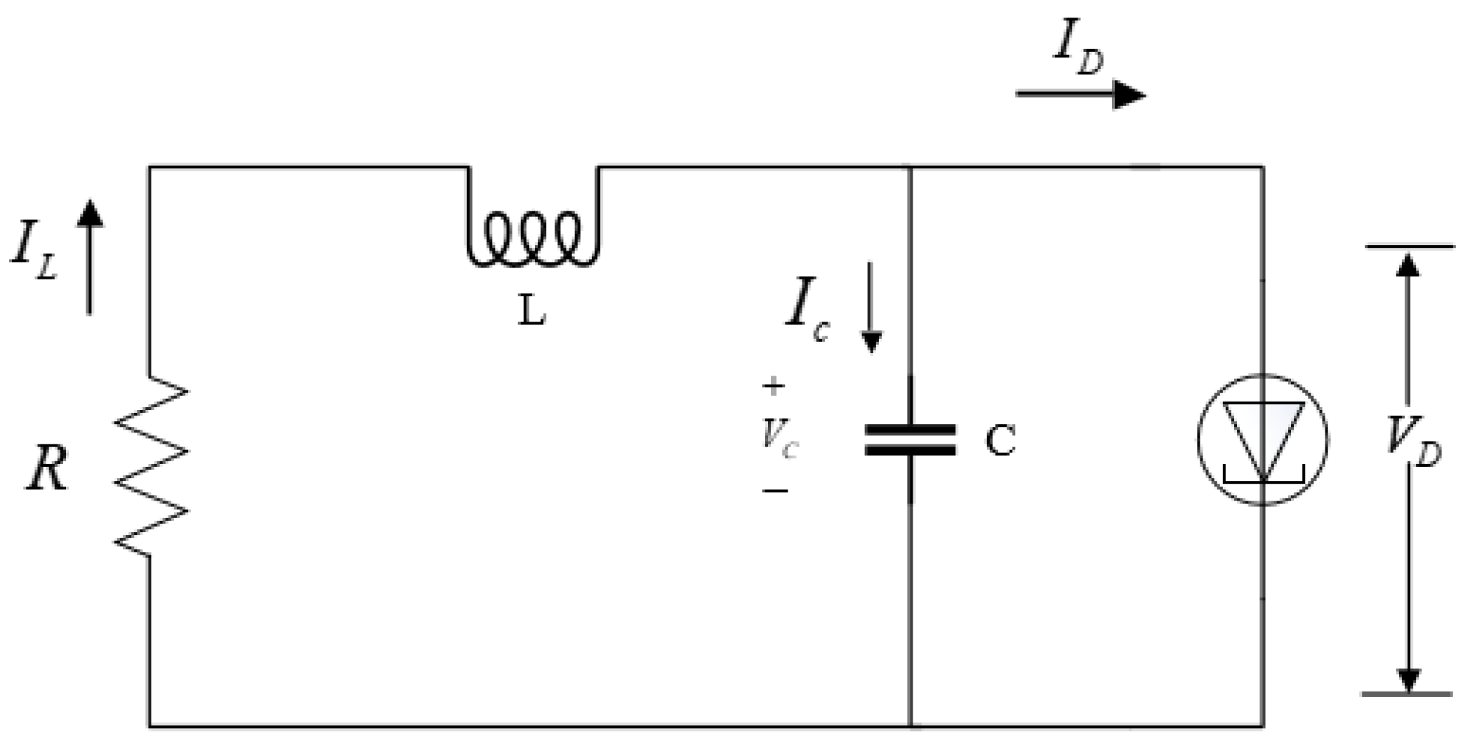
Firstly, consider and modify the case of a tunnel diode circuit in [31], as shown in Figure 1, which is characterized by $I_D=0.002V_D\left(t\right)+0.01V_D^3\left(t\right).$ Let ${\chi }_1\left(t\right)=V_c\left(t\right)$, ${\chi }_2\left(t\right)=I_L\left(t\right)$. The following equation is given,

$$\begin{array}{c}C{\chi }_1(t+1)=-0.002{\chi }_1\left(t\right)-0.01{\chi }_1^3\left(t\right)+0.3999*{10}^{-3}{\chi }_2\left(t\right),\hfill \\ L{\chi }_2(t+1)=-{\chi }_1\left(t\right)-R{\chi }_2\left(t\right)+w\left(t\right),\hfill \end{array}$$

(18)

where $w\left(t\right)$ is the disturbance noise input, C is the capacitance, L is the inductance, and R is the resistance.

In order to facilitate the analysis, we use as few rules as possible. The following two rules are used to approximate the nonlinear systems,

$$\begin{array}{c}PlantRule1:IF\zeta \left(t\right)\in {\xi }_1\left(\zeta \left(t\right)\right),THEN:\hfill \\ {\chi }_1(t+1)=-\frac{0.02}{C_1}{\chi }_1\left(t\right)-\frac{0.01}{C_1}{\chi }_1^3\left(t\right)+\frac{0.3999*{10}^{-3}}{C_1}{\chi }_2\left(t\right)\hfill \\ {\chi }_2(t+1)=-\frac{1}{L_1}{\chi }_2\left(t\right)-\frac{R}{L_1}{\chi }_2\left(t\right)+w\left(t\right)\hfill \end{array}$$

$$\begin{array}{c}PlantRule2:IF\zeta (t)\in {\xi }_2\left(\zeta (t)\right),THEN:\hfill \\ {\chi }_1(t+1)=-\frac{0.02}{C_2}{\chi }_1\left(t\right)-\frac{0.01}{C_2}{\chi }_1^3\left(t\right)+\frac{0.3999*{10}^{-3}}{C_2}{\chi }_2\left(t\right)\hfill \\ {\chi }_2(t+1)=-\frac{1}{L_2}{\chi }_2\left(t\right)-\frac{R}{L_2}{\chi }_2\left(t\right)+w\left(t\right)\hfill \end{array}$$

Taking into account the system error when the linear system approximates the nonlinear system, it is substituted into the model in the form of a model error; then, the matrix parameters are:

$$\begin{array}{c}{A}_{11}\left({\epsilon }_t\right)=\left[\begin{array}{cc}\frac{0.02}{C_1}& R+\mathsf{\Delta }{\epsilon }_t\\ 0& \frac{0.02}{C_1}\end{array}\right],\hfill \\ A_{12}\left({\epsilon }_t\right)=\left[\begin{array}{cc}\frac{0.02}{C_1}& R+\mathsf{\Delta }{\epsilon }_t\\ 0& \frac{0.02}{C_1}\end{array}\right],\hfill \\ B_{11}\left({\epsilon }_t\right)=B_{12}\left({\epsilon }_t\right)=\left[\begin{array}{cc}\frac{R}{L_1}& 0\\ 0& \frac{R}{L_1}\end{array}\right],\hfill \\ A_{21}\left({\epsilon }_t\right)=\left[\begin{array}{cc}\frac{0.02}{C_2}& \mathrm{R}+\mathsf{\Delta }{\epsilon }_t\\ 0& \frac{0.02}{C_2}\end{array}\right],\hfill \\ A_{22}\left({\epsilon }_t\right)=\left[\begin{array}{cc}\frac{0.02}{C_2}& \mathrm{R}+\mathsf{\Delta }{\epsilon }_t\\ 0& \frac{0.02}{C_2}\end{array}\right],\hfill \\ B_{21}\left({\epsilon }_t\right)=B_{22}\left({\epsilon }_t\right)=\left[\begin{array}{cc}\frac{R}{L_2}& 0\\ 0& \frac{R}{L_2}\end{array}\right],\hfill \end{array}$$

and the numerical values in the simulation experiment are $C_1\in \left[0.2F,0.25F\right],C_2\in \left[0.4F,0.45F\right]$, $L_1\approx 1H,L_2\approx 1.2H,R=0.0196\mathsf{\Omega }.$ Then, the matrix parameters are as follows, where the parameter before the model error, ${\epsilon }_t$, is adjustable, which represents the “size” of the uncertainty:

$$\begin{array}{c}{A}_{11}\left({\epsilon }_t\right)=\left[\begin{array}{cc}0.9802& 0.0196+0.99{\epsilon }_t\\ 0& 0.9802\end{array}\right],\hfill \\ A_{12}\left({\epsilon }_t\right)=\left[\begin{array}{cc}0.9904& 0.0196+0.99{\epsilon }_t\\ 0& 0.9904\end{array}\right],\hfill \\ B_{11}\left({\epsilon }_t\right)=B_{12}\left({\epsilon }_t\right)=\left[\begin{array}{cc}0.0196& 0\\ 0& 0.0196\end{array}\right],\hfill \\ C_{11}\left({\epsilon }_t\right)=C_{12}\left({\epsilon }_t\right)=\left[\begin{array}{cc}1& 0\\ 0& 1\end{array}\right],D_{11}\left({\epsilon }_t\right)=D_{12}\left({\epsilon }_t\right)=\left[\begin{array}{cc}1& -1\end{array}\right],\hfill \\ A_{21}\left({\epsilon }_t\right)=\left[\begin{array}{cc}0.4901& 0.0196+0.99{\epsilon }_t\\ 0& 0.4901\end{array}\right],\hfill \\ A_{22}\left({\epsilon }_t\right)=\left[\begin{array}{cc}0.5902& 0.0196+0.99{\epsilon }_t\\ 0& 0.5902\end{array}\right],\hfill \\ B_{21}\left({\epsilon }_t\right)=B_{22}\left({\epsilon }_t\right)=\left[\begin{array}{cc}0.0163& 0\\ 0& 0.0163\end{array}\right],\hfill \\ C_{21}\left({\epsilon }_t\right)=C_{22}\left({\epsilon }_t\right)=\left[\begin{array}{cc}1& 0\\ 0& 1\end{array}\right],D_{21}\left({\epsilon }_t\right)=D_{22}\left({\epsilon }_t\right)=\left[\begin{array}{cc}1& -1\end{array}\right],\hfill \\ Q_{l,t}=\left[\begin{array}{cc}1.9608& 0.0195\\ 0.0195& 1.9605\end{array}\right],R_{l,t}=1.00000,{\Pi }_{l,0}=\left[\begin{array}{cc}1& 0\\ 0& 1\end{array}\right].\hfill \end{array}$$

Given the transition probability matrix, ${\pi }_{a,b}=\left[\begin{array}{cc}0.2& 0.8\\ 0.5& 0.5\end{array}\right]$.

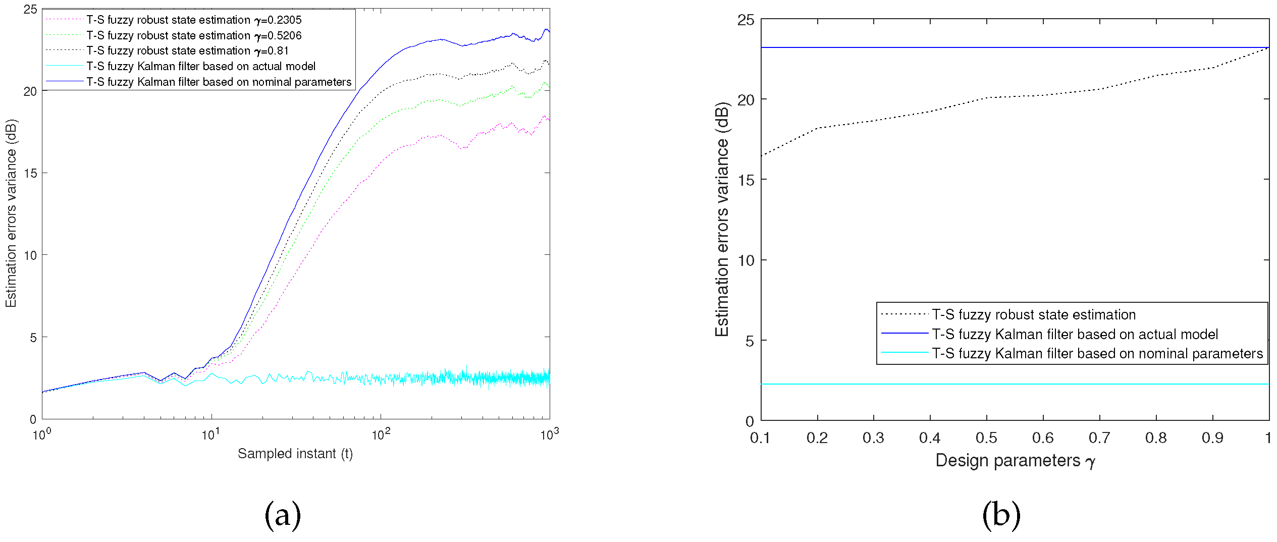
In the first group of simulations, the model error, ${\epsilon }_t$, is fixed at −0.8508, and the deterministic input, $u\left(t\right)$, is also fixed at $u\left(t\right)=\left[1.0;0.1\right]$. Figure 2a shows the estimation error variances with respect to the time samples and the T–S fuzzy state estimator design parameter, γ. It can be clearly seen that when the design parameter, γ, is about 0.2; the performance of the T–S fuzzy state estimator proposed in this paper is about 12 dB different from that of the T–S fuzzy Kalman filter based on the actual parameters, but the performance is improved by nearly 10 dB compared with that of the T–S fuzzy Kalman filter based on the nominal parameters. The same conclusion can be drawn from Figure 2b.

Figure 2b shows that, at the sampled instant t = 500, if γ takes any value between 0.1 and 1.0, the performance of the derived T–S fuzzy robust state estimator is better than that of the T–S fuzzy Kalman filter based on the nominal parameter values.

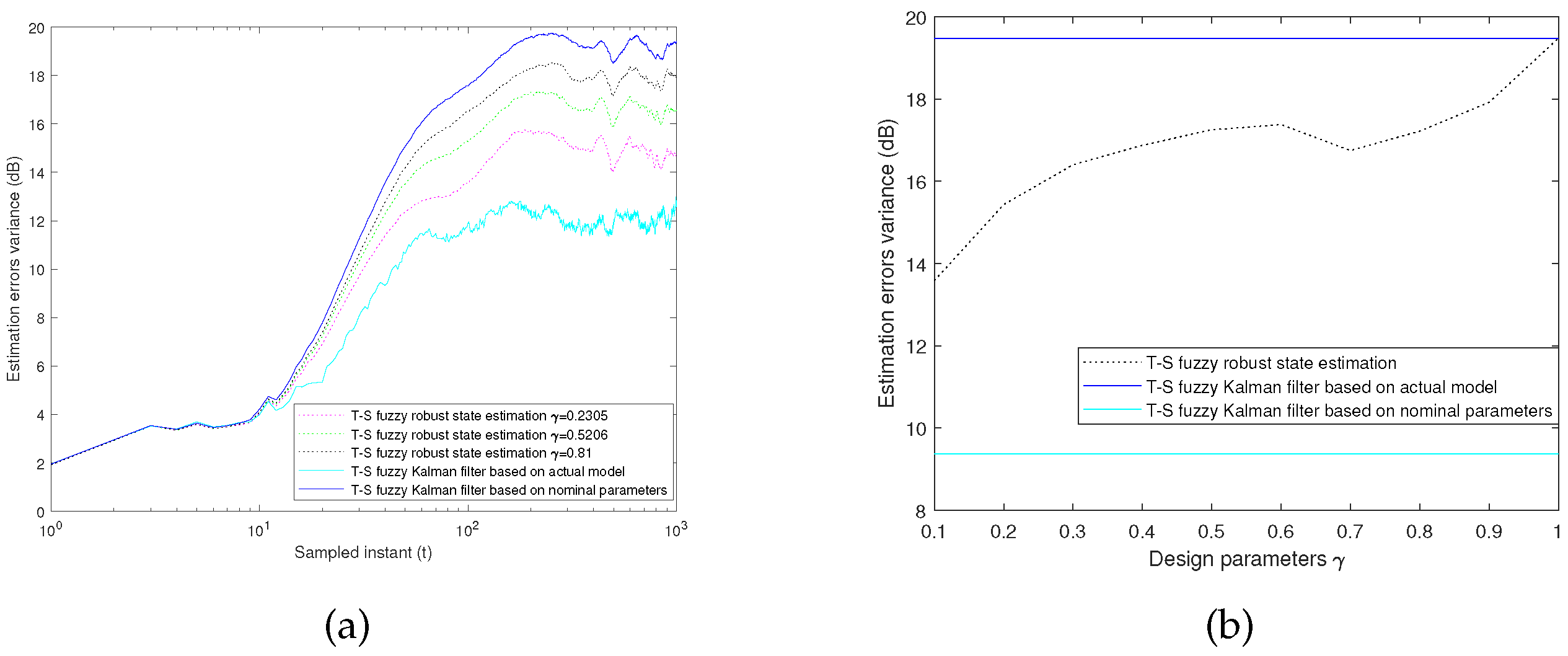
In the second group of simulations, the uncertainty of the system model is increased, that is, the model error, ${\epsilon }_t$, changes randomly. The model error is generated by the intercept of the Gaussian distribution, and the mean value is set to 0 and the variance is set to 1, while the external input signals, $u\left(t\right)$, are fixed to $\left[1.0;0.1\right]$. In addition, the amplitude of the model error cannot be greater than 1. If the given requirement is not met, it is deleted and regenerated until the amplitude satisfies less than 1.

From Figure 3b, we can see that there exists a large interval of γ, which leads to the T–S fuzzy robust estimator with better performance than the T–S fuzzy Kalman filter, based on the nominal parameters at the sampled instant t = 500.

The two sets of simulation cases show that the derived fuzzy robust state estimator performs satisfactorily compared to ignoring uncertain estimators under fuzzy rules and the Markov jump strategy. This means that the proposed method is an effective state estimation method in practical engineering.

6. Conclusions

In this paper, a fuzzy robust state estimator is designed for a class of nonlinear systems with sudden changes in the system structure and parameters due to external disturbances. Firstly, based on Markov jump strategy, the T–S fuzzy method is used to model the nonlinear system, and the inevitable deviation of the linear subsystem when approaching the nonlinear is taken into account, which is expressed as the model error in system modeling. Secondly, the robust state estimation method, based on the sensitivity penalty, is used to design sub-estimators for uncertain linear subsystems, and fuzzy robust state estimators for nonlinear systems are obtained by fuzzy rules and membership functions. Thirdly, the steady state analysis of the proposed fuzzy state estimator is given under certain conditions. Finally, the numerical simulation of a tunnel diode circuit proves that the proposed fuzzy robust state estimator has good state estimation performance.

References

Wang, J.; Mao, Y.; Li, Z.; Gao, J.; Liu, H. Robust state estimation for uncertain linear discrete systems with d-step state delay. IET Control Theory Appl.2021, 40, 1708–1723. [Google Scholar] [CrossRef]
Liu, H.; Zhou, T. Robust state estimation for uncertain linear systems with random parametric uncertainties. Sci. China Inform. Sci.2018, 60, 012202. [Google Scholar] [CrossRef]
Dong, S.; Wu, Z.-G.; Shi, P.; Su, H. Reliable control of fuzzy systems with quantization and switched actuator failures. IEEE Trans. Cybern.2017, 15, 2198–2208. [Google Scholar] [CrossRef]
Chao, C.; Chen, D.; Chiou, J. Stability Analysis and Robust Stabilization of Uncertain Fuzzy Time-Delay Systems. Mathematics2021, 9, 2441. [Google Scholar] [CrossRef]
Huang, S.; Yang, G. Fault estimation for fuzzy delay systems: A minimum norm least squares solution approach. IEEE Trans. Cybern.2017, 47, 2389–2399. [Google Scholar] [CrossRef]
Sun, J.; Zhang, H.; Wang, Y. Dissipativity analysis on switched uncertain nonlinear T-S fuzzy Systems with stochastic perturbation and time delay. J. Frankl. Inst.2020, 357, 13410–13429. [Google Scholar] [CrossRef]
Li, Z.; Wang, J.; Liu, H. A robust state estimator for T-S fuzzy system. IEEE Access2020, 8, 84063–84069. [Google Scholar] [CrossRef]
Li, H.; Yin, S.; Liu, J.; Zhao, C. Novel Gaussian approximate filter method for stochastic nonlinear system. Int. J. Innov. Comput. Inf. Control2017, 13, 201–218. [Google Scholar]
Sun, K.; Shuai, S.; Tong, S. Fuzzy Adaptive Decentralized Optimal Control for Strict Feedback Nonlinear Large-Scale Systems. IEEE Trans. Cybern2018, 48, 1326–1339. [Google Scholar] [CrossRef]
Luo, Y.; Alsaadi, F.E. Robust H∞ filtering for a class of two-dimensional uncertain fuzzy systems with randomly occurring mixed delays. IEEE Trans. Fuzzy Syst.2017, 25, 70–83. [Google Scholar] [CrossRef]
Jiang, B.; Kao, Y.; Gao, C. Passification of uncertain singular semi-Markovian jump systems with actuator failures via sliding mode approach. IEEE Trans. Autom. Control2017, 62, 4138–4143. [Google Scholar] [CrossRef]
Sala, A.; Hernández-Mejías, M.; Arino, C. Stable receding-horizon scenario predictive control for Markov-jump linear systems. Automatica2017, 86, 121–128. [Google Scholar] [CrossRef]
Li, F.; Shi, P.; Wu, L.; Basin, M.V.; Lim, C.-C. Quantized control design for cognitive radio networks modeled as nonlinear semiMarkovian jump systems. IEEE Trans. Ind. Electron.2015, 62, 2330–2340. [Google Scholar] [CrossRef]
Wu, Z.; Dong, S. Fuzzy-model-based nonfragile guaranteed cost control of nonlinear Markov jump systems. IEEE Trans. Syst. Man. Cybern.2017, 47, 2388–2397. [Google Scholar] [CrossRef]
Morais, C.F.; Palma, J.M.; Peres, P.L.D.; Oliveira, R.C.L.F. An LMI approach for H2 and H∞ reduced-order filtering of uncertain discrete-time Markov and Bernoulli jump linear systems. Automatica2018, 95, 463–471. [Google Scholar] [CrossRef]
Gorynin, I.; Derrode, S.; Monfrini, E.; Pieczynski, W. Fast filtering in switching approximations of nonlinear Markov systems with applications to stochastic volatility. IEEE Trans. Autom. Control2017, 62, 853–862. [Google Scholar] [CrossRef]
Li, X.; Lam, J.; Gao, H.; Xiong, J. H∞ and H2 filtering for linear systems with uncertain Markov transitions. Automatica2016, 67, 252–266. [Google Scholar] [CrossRef]
Wu, Z.; Shi, P.; Su, H.; Lu, R. Asynchronous l2 -l∞ filtering for discrete-time stochastic Markov jump systems with randomly occurred sensor nonlinearities. Automatica2014, 50, 180–186. [Google Scholar] [CrossRef]
Zhu, Y.; Zhang, L.; Zheng, W. Distributed H∞ filtering for a class of discrete-time Markov jump Lur’e systems with redundant channels. IEEE Trans. Ind. Electron.2016, 63, 1876–1885. [Google Scholar] [CrossRef]
Zhang, M.; Shi, P. Quantized Feedback Control of Fuzzy Markov Jump Systems. IEEE Trans. Cybern.2019, 49, 3375–3384. [Google Scholar] [CrossRef] [PubMed]
Zhang, M.; Shi, P. Network-based fuzzy control for nonlinear Markov jump systems subject to quantization and dropout compensationy. Fuzzy Sets Syst.2019, 371, 96–109. [Google Scholar] [CrossRef]
Yin, Y.; Shi, P. Robust filtering for nonlinear nonhomogeneous Markov jump systems by fuzzy approximation approach. IEEE Trans. Cybern.2015, 45, 1706–1716. [Google Scholar] [CrossRef] [PubMed]
Tao, J.; Lu, R.; Shi, P.; Su, H.; Wu, Z. Dissipativity-based reliable control for fuzzy Markov jump systems with actuator faults. IEEE Trans. Cybern.2017, 47, 2377–2388. [Google Scholar] [CrossRef] [PubMed]
Zhang, L.; Ning, Z.; Shi, P. Input–output approach to control for fuzzy Markov jump systems with time-varying delays and uncertain packet dropout rate. IEEE Trans. Cybern2015, 45, 2449–2460. [Google Scholar] [CrossRef]
Liu, H.; Zhou, T. Robust state estimation for uncertain linear systems with deterministic input signals. Control Theory Technol.2014, 12, 383–392. [Google Scholar] [CrossRef]
Meng, F.; Gao, J.; Liu, H. Robust State Estimation for Time-Delay Linear Systems With External Inputs. IEEE Access2021, 9, 106540–106549. [Google Scholar] [CrossRef]
Zhou, T. Sensitivity penalization based robust state estimation for uncertain linear systems. IEEE Trans. Autom. Control2010, 55, 1018–1024. [Google Scholar] [CrossRef]
Tseng, C. Fuzzy tracking control design for nonlinear dynamic systems via T-S fuzzy model. IEEE Trans. Fuzzy Syst.2001, 9, 381–392. [Google Scholar] [CrossRef] [Green Version]
Zhou, T.; Liang, H. On asymptotic behaviors of a sensitivity penalization based robust state estimator. Syst. Control Lett.2011, 60, 174–180. [Google Scholar] [CrossRef]
Nguang, S.; Assawinchaichote, W. H∞ filtering for fuzzy dynamical systems with D stability constraints. IEEE Trans. Circuits Syst. I Fundam. Theory Appl.2003, 50, 1503–1508. [Google Scholar] [CrossRef]
Figure 1.
Tunnel diode circuit.
Figure 2.
The model error, , is fixed. (a) The design parameter, γ, is fixed. (b) The sampled instant, t, is fixed.
Figure 3.
The model error, , is not fixed. (a) The design parameter, γ, is fixed. (b) The sampled instant, t, is fixed.
Disclaimer/Publisher’s Note: The statements, opinions and data contained in all publications are solely those of the individual author(s) and contributor(s) and not of MDPI and/or the editor(s). MDPI and/or the editor(s) disclaim responsibility for any injury to people or property resulting from any ideas, methods, instructions or products referred to in the content.
Zhang, Z.; Wang, J.; Gao, J.; Liu, H.