Mixed-Integer Conic Formulation of Unit Commitment with Stochastic Wind Power

Abstract

Due to the high randomness and volatility of renewable energy sources such as wind energy, the traditional thermal unit commitment (UC) model is no longer applicable. In this paper, in order to reduce the possible negative effects of an inaccurate wind energy forecast, the chance-constrained programming (CCP) method is used to study the UC problem with uncertainty wind power generation, and chance constraints such as power balance and spinning reserve are satisfied with a predetermined probability. In order to effectively solve the CCP problem, first, we used the sample average approximation (SAA) method to transform the chance constraints into deterministic constraints and to obtain a mixed-integer quadratic programming (MIQP) model. Then, the quadratic terms were incorporated into the constraints by introducing some auxiliary variables, and some second-order cone constraints were formed by combining them with the output characteristics of thermal unit; therefore, a tighter mixed-integer second-order cone programming (MISOCP) formulation was obtained. Finally, we applied this method to some systems including 10 to 100 thermal units and 1 to 2 wind units, and we invoked MOSEK in MATLAB to solve the MISOCP formulation. The numerical results obtained within 24 h confirm that not only is the MISOCP formulation a successful reformulation that can achieve better suboptimal solutions, but it is also a suitable method for solving the large-scale uncertain UC problem. In addition, for systems of up to 40 units within 24 h that do not consider wind power and pollution emissions, the numerical results were compared with those of previously published methods, showing that the MISOCP formulation is very promising, given its excellent performance.

1. Introduction

1.1. Motivation and Incitement

Unit commitment (UC) in a power system is an important aspect of optimization that has been studied for a long time. It determines the on–off status and outputs of generation units over a scheduling planning horizon while minimizing the total operational cost of the system [1,2,3,4]. In recent years, owing to the dramatic reduction in fossil fuels and the increased demand for cleaner energy, renewable energy sources such as wind and solar energy have attracted widespread attention, with significantly increased used in power systems [5]. As a typical representative of renewable energy, the use of wind energy has rapidly increased, and it is considered one of the most promising alternative energies. However, wind energy has a strong randomness and uncertainty and is usually difficult to accurately predict. The implementation of large-scale wind power brings many difficulties to the operation of a power system. Therefore, it is worth establishing rapid and effective solutions to the thermal UC problem, in combination with wind generation. In this paper, a mixed-integer second-order conic programming formulation of chance-constrained UC with wind power uncertainty is proposed, which can be effectively solved by related software. The proposed method is suitable for solving the large-scale uncertain UC problem.

1.2. Literature Review

The thermal UC problem is usually modeled as a large-scale mixed-integer non-linear program in mathematics [6], and it can be effectively solved by the metaheuristic method [7], Lagrange relaxation method [8], outer approximation method [9], etc. In recent years, as an increasing number of renewable energy generations have been incorporated into power systems, the related UC model has become increasingly complex and random, and the related problem has become more difficult to effectively solve. With the creation of stochastic optimization algorithms that achieve good numerical performance, the number of published studies addressing renewable energy generation in the thermal UC problem has increased. Zhu et al. [10] presented a stochastic programming model for the related UC problem, and the uncertainties of renewable energy generation were thoroughly simulated in the form of synthetic ensemble forecasts and scenario trees. Vatanpour and Yazdankhah [11] also presented a stochastic security constrained UC model that included a wind power farm and energy storage systems, and the problem was solved by a scenario-based method that incorporated the Benders decomposition technique. Shahbazitabar and Abdi [12] considered a stochastic UC model with an electric vehicle parking plot, and a priority-list-based heuristic method was used to solve the model. However, these scenario-based methods require a large number of scenarios to achieve high accuracy. As a result, the related mathematical models are very large and difficult to solve. To address this problem, some robust models have been proposed by researchers for the related UC problem. Zhou et al. [13] presented a robust UC model for a hybrid AC/DC power system in which the problem was formulated as mixed-integer second-order cone programming with a data-adaptive uncertainty set, and extreme scenarios were introduced to reformulate the robust optimization. Sun et al. [14] presented an optimal day-ahead wind–thermal generation-scheduling method that considered the statistical and predicted features of wind speeds. Ref. [15] proposed a data-driven adaptive robust optimization (ARO) framework for the UC problem integrating wind power, and the model was formulated as a four-level optimization problem to be solved. However, the conservatism of these robust optimization methods needs to be improved.

Chance-constrained programming (CCP) is an effective method for solving the stochastic problem that has been applied to the relevant UC problem. Ref. [16] proposed a chanced-constrained model for the related UC with high wind energy penetration and used two approximation approaches—the quantile-based approximation approach and p-efficient point—to solve CCP. Ref. [17] proposed a chance-constrained UC model to guarantee the utilization of wind power, and the chance constraints were transformed into sample average reformulations by the sample average approximation algorithm. Ref. [18] presented a chance-constrained two-stage stochastic programming UC problem that considers the uncertainties of loads and wind power, and the problem was converted into an equivalent deterministic formulation by a sequence of approximations and verification. In ref. [19], a Gaussian mixture model was used to deal with wind power forecast errors, and the Newton method was proposed to obtain the quantiles and transform chance constraints into deterministic constraints. In these studies, the outputs of wind power generation are considered random variables with a probability distribution, and CCP ensures that the probability of the constraints with random variables is not less than a given confidence level. However, with respect to the uncertainty of wind power output, there are still two major challenges associated with solving the CCP formulation. One is that an accurate probabilistic model of random variables is needed; the other is how it efficiently transforms the chance constraint into an equivalent deterministic formulation.

1.3. Contribution and Paper Organization

It is very difficult to directly solve CCP, and a popular technique is to transform it into a deterministic formulation via a sample average approximation (SAA). Ref. [20] reformulated the chance constraints as mixed-integer non-linear programming; the integer variables were relaxed into continuous variables and regularized by expanding the feasible region. Ref. [21] reviewed recent developments in mixed-integer linear formulations of CCP with finite discrete distributions. In this paper, we consider the CCP model of the UC problem with the uncertainty of wind power output, which addresses stochastic wind power output by introducing chance constraints. An equivalent mixed-integer second-order conic reformulation of an original chance-constrained UC model is derived. The main contributions of this paper are summarized as follows.

(i)

By introducing some auxiliary variables, the quadratic terms in objective function are incorporated into the constraints, and some rotating second-order cone constraints with better compactness are obtained, which combine the constraint characteristics, such as the upper and lower bounds of thermal unit output.

(ii)

Using the SAA method, we derive a mixed-integer formulation of a chance-constrained model of the considered UC problem with finite discrete distributional information. Then, an equivalent deterministic reformulation for the related UC problem is obtained, which can be readily solved with state-of-the-art optimization software.

(iii)

The proposed method is tested on systems that contain between 10 and 100 thermal units and 1 to 2 wind units, and the deterministic reformulation is solved by MOSEK in MATLAB. The simulation results show that the presented method is suitable for the large-scale stochastic chance-constrained UC problem.

The remainder of this paper is organized as follows. In Section 2, the chance-constrained model of the stochastic UC problem with wind power is introduced. The solution procedure is described in Section 3. Numerical tests and simulation results are presented to illustrate the performance of the proposed method in Section 4. The maximum penetration rate of wind power analysis and a discussion of practical implementation are provided in Section 5. Conclusions are drawn in Section 6.

2. Mathematical Formulation of Chance-Constrained UC

2.1. Objective Function

The UC problem with stochastic wind power consists of thermal generators and wind power farms. The objective of the related UC problem is to acquire the optimal on–off schedule and output for thermal generators over the scheduled time horizon so that the overall operation cost can be minimized. The overall operation cost consists of three parts and can be expressed as follows:

$$\min F_C=f_1\left(P_{i,t}\right)+f_2\left(P_{i,t}\right)+S_{i,t}$$

(1)

where the fuel cost is $f_1\left(P_{i,t}\right)={\sum }_{i=1}^N{\sum }_{t=1}^T[{\alpha }_i{u}_{i,t}+{\beta }_i{P}_{i,t}+{\gamma }_i{\left(P_{i,t}\right)}^2]$; the pollutant emission cost is $f_2\left(P_{i,t}\right)={\sum }_{t=1}^T{\sum }_{i=1}^N[a_i{u}_{i,t}+b_i{P}_{i,t}+c_i{(P_{i,t})}^2]$; and the startup cost ($S_{i,t}$) is incurred when a thermal unit is put into operation, which depends on how long the unit has been inactive, i.e., $S_{i,t}$ only depends on the binary variable associated with the on/off state of generating units. The startup cost ($S_{i,t}$) can be approximated by the following linearization inequalities [1,2]:

$$\{\begin{array}{c}{S}_{i,t}\ge k_{i,\tau }\left[u_{i,t}-{\sum }_{j=1}^{\tau }{u}_{i,t-j}\right]\hfill \\ S_{i,t}\ge 0,i=1,\cdots ,N;t=1,\cdots ,T;\tau =1,\cdots ,N_{D,i}\hfill \end{array}$$

(2)

where $N_{D,i}$ is a given parameter, and the coefficient $k_{i,\tau }$ is represented by the following piecewise function:

$$k_{i,\tau }=\{\begin{array}{c}{C}_{hot,i }, \tau =1,\cdots ,{\underset{\_}{T}}_{off,i}+T_{cold,i}\hfill \\ C_{cold,i }, \tau ={\underset{\_}{T}}_{off,i}+T_{cold,i+1},\cdots ,N_{D,i}\hfill \end{array}$$

It is worth noting that the objective function (1) can be assigned different weighting factors according to the importance of each cost.

2.2. Constraints

The UC problem with wind power uncertainty essentially involves system chance constraints and thermal generator constraints; the physical constraints for thermal generators are described in detail in Ref. [1]. The mathematical expression of these constraints are as follow:

(1) Power balance chance constraint:

$$Pr\left\{{\sum }_{i=1}^N{P}_{i,t}+{\sum }_{j=1}^{Nw}{P}_{\xi ,t}{}^j\ge P_{D,t}\right\}\ge 1-\epsilon$$

(3)

where the random variable $P_{\xi ,t}{}^j$ is the actual wind power output value of wind unit $j$ at time period $t$, and $\epsilon \in \left(0,1\right)$ is a given confidence level. Due to the randomness of wind power, it must be guaranteed with a high probability for the power balance of the power system.

(2) Spinning reserve chance constraint:

$$Pr\{{\sum }_{i=1}^N{u}_{i,t}{\overline{P}}_i+{\sum }_{j=1}^{Nw}{P}_{\xi ,t}{}^j\ge P_{D,t}+R_t\}\ge 1-\epsilon$$

(4)

which is necessary in the operation of a power system. If the load is interrupted or suddenly increases, the power quality is guaranteed by the maximum available capacity of the active thermal units.

(3). Thermal generator output constraint:

$$u_{i,t}{\underset{\_}{P}}_i\le P_{i,t}\le u_{i,t}{\overline{P}}_i$$

(5)

which represents the output value of thermal unit $i$ at time period $t$ and must be limited to a certain range.

(4) Thermal generator ramping-up rate constraint:

$$P_{i,t}-P_{i,t-1}\le u_{i,t}(P_{up,i}+{\underset{\_}{P}}_i)-u_{i,t-1}{\underset{\_}{P}}_i+s_{i,t}(P_{start,i}-P_{up,i}-{\underset{\_}{P}}_i)$$

(6)

(5) Thermal generator ramping-down rate constraint:

$$P_{i,t-1}-P_{i,t}\le u_{i,t-1}\left(P_{down,i}+{\underset{\_}{P}}_i\right)-u_{i,t}{\underset{\_}{P}}_i+d_{i,t}(P_{shut,i}-P_{down,i}-{\underset{\_}{P}}_i)$$

(7)

The power output of a thermal unit cannot fluctuate too rapidly, and the ramp-up/down rate reflects the maximum load increase/decrease in the two successive time periods.

(6) Thermal generator minimum uptime constraint:

$${\sum }_{\overline{\omega }={[t-{\underset{\_}{T}}_{on,i}]}^{+}+1}^t{s}_{i,\overline{\omega }}\le u_{i,t},t\in \left[U_i+1,\dots ,T\right]$$

(8)

where $U_i=\left[\min \right[T,u_{i,0}\left({\underset{\_}{T}}_{on,i}-T_{i,0}\right)]{]}^{+}$, and ${\left[a\right]}^{+}=\max \left[0,a\right]$.

(7) Thermal generator minimum downtime constraint:

$${\sum }_{\overline{\omega }={[t-{\underset{\_}{T}}_{off,i}]}^{+}+1}^t{d}_{i,\overline{\omega }}\le 1-u_{i,t},t\in \left[L_i+1,\dots ,T\right]$$

(9)

where $L_i=\left[\min \right[T,u_{i,0}\left({\underset{\_}{T}}_{off,i}+T_{i,0}\right)]{]}^{+}$. Constraints (8) and (9) indicate that the thermal generators must remain in the on/off state for several consecutive time periods after startup/shutdown.

(8) State constraint:

$$s_{i,t}-d_{i,t}=u_{i,t}-u_{i,t-1}$$

(10)

Based on the analysis presented above, the mathematical model of the UC problem with wind power uncertainty can be expressed as the following chance-constrained program:

$$\begin{array}{c}\min F_c={\sum }_{i=1}^N{\sum }_{t=1}^T\left[({\alpha }_i+a_i)u_{i,t}+({\beta }_i+b_i)P_{i,t}+({\gamma }_i+c_i)){\left(P_{i,t}\right)}^2+S_{i,t}\right] \\ \left(2\right)-\left(10\right)\\ u_{i,t},s_{i,t}, d_{i,t}\in \left\{0,1\right\}, P_{i,t},S_{i,t}\ge 0, P_{\xi ,t}{}^j\ge 0 \mathrm{is} \mathrm{a} \mathrm{random} \mathrm{variable} ,i\in N,t\in T \end{array}\}$$

(11)

Chance constraints (3) and (4) of wind power uncertainties are vital for (11), but it is difficult to solve these. In this paper, the SAA method is employed to solve the chance constraints, and the chance-constrained model (11) can be transformed into an equivalently and deterministically mixed-integer quadratic program. Furthermore, it can be reformulated as a mixed-integer second-order conic problem by introducing some auxiliary variables.

3. Solution Procedure

3.1. Deterministic Reformulation of Chance Constraints

For the sake of convenience and a given probability space $\left(\mathsf{\Omega },ℱ,\mathcal{P}\right)$, we take the following chance-constrained program (CCP) as an example to introduce the basic ideas of deterministic reformulation [21].

$$\begin{gathered} \min c^{T}x \\ s.t.P_r\left\{x\in \rho \left(\xi \right)\right\}\ge 1-\epsilon \\ x\in X \end{gathered}$$

(12)

where $c\in R^n$ is the coefficient vector of the objective function, $\xi \in \mathsf{\Omega }$ is a random vector with a known distribution ($\mathcal{P}$), $\epsilon \in \left(0,1\right)$ is a confidence level given by the decision maker, $X\subset R^n$ is a compact set, and the polyhedron $\rho \left(\xi \right)$ is the set of solutions that are safe or desirable. Let

$$\rho \left(\xi \right)≔\{x| Tx\ge r\left(\xi \right)\}$$

(13)

where $T$ is an $m\times n$ deterministic matrix, and $r\left(\xi \right)$ is a random column vector in $R^m$.

Consider CCP (12) under a finite discrete probability space; the true distribution can be approximated by finite empirical distribution. For ease of description, we assume that the K samples are independent and identically distributed and consider the following SAA formulation of CCP (12):

$$\begin{gathered} \min c^{T}x \\ s.t. \frac{1}{K}{\sum }_{k=1}^K\mathsf{\Theta }\left(x\notin \rho \left({\xi }_k\right)\right)\le \epsilon \\ x\in X \end{gathered}$$

(14)

where $\mathsf{\Theta }(.)$ is an indicator function and equals 0 or 1. From the formulation (14), it is evident that the use of finite discrete distribution avoids the difficulty of assessing the probability when the distribution is not precisely given. Under non-equal probability scenarios, the part I constraint of (14) is simply:

$${\sum }_{k=1}^K{p}_k\mathsf{\Theta }\left(x\notin \rho \left({\xi }_k\right)\right)\le \epsilon$$

By introducing binary variables ($z_k\left(k=1,\dots ,K\right)$) and letting $Tx=t$, the Formulation (14) can be transformed into the following mixed-integer linear program (MILP):

$$\begin{gathered} \min c^{T}x \\ s.t. \begin{array}{c}\begin{array}{c}x\in X,Tx-t=0\\ t_j+r\left({\xi }_k^j\right)z_k\ge r\left({\xi }_k^j\right),\forall k=1,\dots ,K,\forall j=1,\dots ,m\\ \frac{1}{K}{\sum }_{k=1}^K{z}_k\le \epsilon \end{array}\\ z\in {\left\{0,1\right\}}^K \end{array}\} \end{gathered}$$

(15)

Because (15) contains big-M constraints ($t_j+r\left({\xi }_k^j\right)z_k\ge r\left({\xi }_k^j\right),\forall k=1,\dots ,K,\forall j=1,\dots ,m$), it is NP-hard. Therefore, it is necessary to obtain the strengthening formulation of SAA to scale up the problem size. An important substructure in this formulation (15) is given for a fixed $j$. Let the following mixed set with cardinality constraint be

$${ℳ}_C≔\{\left(t_j,z\right)\in R_{+}\times {\left\{0,1\right\}}^K:t_j\ge r\left({\xi }_k^j\right)\left(1-z_k\right),\frac{1}{K}{{\displaystyle \sum }}_{k=1}^K{z}_k\le \epsilon ,\forall k=1,\dots ,K\}$$

Sort the values of $r\left({\xi }_k^j\right)$ for $k \left(k=1,\dots ,K\right)$ to obtain a permutation (σ) such that

$$r\left({\xi }_{{\sigma }_1}^j\right)\ge r\left({\xi }_{{\sigma }_2}^j\right)\ge \dots \ge r\left({\xi }_{{\sigma }_{\mathrm{K}}}^j\right)$$

By reason of the cardinality constraint ($\frac{1}{K}{\sum }_{k=1}^K{z}_k\le \epsilon$), we have $t_j\ge r\left({\xi }_{{\sigma }_{\mathrm{k}+1}}^j\right)$; then, we can replace the inequalities ($t_j\ge r\left({\xi }_k^j\right)\left(1-z_k\right)$) of ${ℳ}_C$ with the following inequalities:

$$t_j+\left[r\left({\xi }_k^j\right)-r\left({\xi }_{{\sigma }_{\mathrm{k}+1}}^j\right)\right]z_k\ge r\left({\xi }_k^j\right), \forall k=1,\dots ,K$$

Consider the subset $\left\{s_1,s_2,\dots ,s_l\right\}\subseteq \left\{{\sigma }_1,{\sigma }_2,\dots ,{\sigma }_q\right\}$ such that $r\left({\xi }_{s_k}^j\right)\ge r\left({\xi }_{s_{k+1}}^j\right)$ for $k=1,2,\dots ,l$, where $q≔\left[K\epsilon \right]$, and $s_1={\sigma }_1,s_{l+1}={\sigma }_{q+1}$. Then, a strong valid inequality for ${ℳ}_C$ is given by

$$t_j+{{\displaystyle \sum }}_{k=1}^l[r\left({\xi }_{s_{\mathrm{k}}}^j\right)-r\left({\xi }_{s_{\mathrm{k}+1}}^j\right)]z_{s_k}\ge r\left({\xi }_{s_1}^j\right)$$

Therefore, the MILP Formulation (15) with big-M constraints can be further transformed as follows:

$$\begin{gathered} \min c^{T}x \\ s.t. \begin{array}{c}\begin{array}{c} x\in X,Tx-t=0\\ t_j+{{\displaystyle \sum }}_{k=1}^l\left[r\left({\xi }_{s_{\mathrm{k}}}^j\right)-r\left({\xi }_{s_{\mathrm{k}+1}}^j\right)\right]z_{s_k}\ge r\left({\xi }_{s_1}^j\right)\\ \frac{1}{K}{{\displaystyle \sum }}_{k=1}^K{z}_k\le \epsilon \end{array}\\ z\in {\left\{0,1\right\}}^K\end{array}\} \end{gathered}$$

(16)

3.2. The Convex Hull Description of a Simple Mixed-Integer Set

It is well known that the main techniques used in computing software for solving integer problems are branch-and-bound and cutting-plane; the tighter the relaxed set, the better the efficiency of the software. Consider the following simple mixed-integer set:

$$C=\left\{\left(s,y,z\right)|s^2-y\le 0, z\underset{\_}{s}\le s\le z\overline{s},0<\underset{\_}{s}<\overline{s} , z\in \left\{0,1\right\}\right\}$$

(17)

where the continuous relaxation of $C$ is

$$C_{CR}=\left\{\left(s,y,z\right)|s^2-y\le 0, z\underset{\_}{s}\le s\le z\overline{s},0<\underset{\_}{s}<\overline{s} , 0\le z\le 1\right\}$$

Evidently, $C\subset C_{CR}$, and $C_{CR}$ is less effective. Refs. [22,23] provide a better set representing the convex hull of $C$:

$$C_{conv}=\left\{\left(s,y,z\right)|s^2-zy\le 0, z\underset{\_}{s}\le s\le z\overline{s},0<\underset{\_}{s}<\overline{s} , y\ge 0, 0\le z\le 1\right\}$$

(18)

Let

$$C_{sub}=\left\{\left(s,y,z\right)|s^2-y\le 0, z\underset{\_}{s}\le s\le z\overline{s},0<\underset{\_}{s}<\overline{s} , 0<z<1\right\}$$

The sets listed above have the following relationship:

$$C_{sub}\subset C_{CR}; C_{sub}{\displaystyle \cap }{C}_{conv}=\varnothing ; C\subset C_{conv}\subset C_{CR}$$

which shows that $C_{conv}$ is a better relaxed set for $C$.

3.3. Scenario Generation

In this subsection, we study the probability distribution of wind power output based on the historical data and first use Monte Carlo sampling technology to generate wind power scenarios. Various probability distribution types of wind power have been discussed in recent years, and the multivariate normal distribution is widely used to construct the probability distribution of random wind power output [24], which can be denoted by $N~\left(\mu ,{\sigma }^2\right)$. The probability distribution function of wind power is defined by

$$f\left(x\right)=\frac{1}{\sigma \sqrt{2\pi }}\exp \left(-\frac{x-\mu }{2{\sigma }^2}\right),-\infty <x<\infty$$

where $\mu =E\left[\xi \right]$ and $\sigma =D\left[\xi \right]$ are the average values and variance of random variables, respectively. Then, a number of wind power scenarios can be generated by Monte Carlo sampling technology with the same probability. For ease of description, we generated 4000 sample points subject to a normal distribution with $\mu =120$ and $\sigma =$ 15; the numerical simulation results are shown in the Figure 1. However, we know that the normal distribution fitted by the Monte Carlo method has considerable variance, as shown in Figure 1. Therefore, we used a Latin hypercube method to generate 4000 sample points, for which the numerical simulation results are shown in the Figure 2. Figure 2 shows that the hypercube method has a better fitting effect [25]. Then, some scenarios with errors can be eliminated, and some typical scenarios can be retained; therefore, the original scenarios are reduced, and the evaluation accuracy is unaffected.

We assumed that the wind power output is subject to multivariate normal distributed, with the hourly forecasted wind power ranging between 0 and 120, which gives a standard deviation of 10% of the expected values. Then, we used Latin hypercube sampling to generate 4000 scenarios for 24 h wind power generation, and the K-means clustering algorithm was employed to classify these scenarios into five types. The corresponding wind power outputs are shown in Figure 3.

Suppose that the probability of each wind power scenario is the same as

$$p_k\left({\xi }_k=P_{\xi ,t}^{j,k}\right)=\frac{1}{K}$$

and the corresponding random variables ($P_{\xi ,t}^j$) in the chance constraints (3), (4) are replaced by $P_{\xi ,t}^{j,k}$ for $1\le k\le K$. Then, the following SAA formulations can be obtained:

$$\frac{1}{K}{\sum }_{k=1}^K\mathsf{\Theta }\left({\sum }_{i=1}^N{P}_{i,t}+{\sum }_{j=1}^{Nw}{P}_{\xi ,t}^{j,k}<P_{D,t}\right)\le \epsilon$$

(19)

$$\frac{1}{K}{\sum }_{k=1}^K\mathsf{\Theta }\left({\sum }_{i=1}^N{u}_{i,t}{\overline{P}}_i+{\sum }_{j=1}^{Nw}{P}_{\xi ,t}^{j,k}<P_{D,t}+R_t\right)\le \epsilon$$

(20)

By introducing some binary variables, (19) and (20) can be reformulated as:

$$\begin{array}{c}\begin{array}{c}{\sum }_{i=1}^N{P}_{i,t}-P_{D,t}+M{z}_k\ge -{\sum }_{j=1}^{Nw}{P}_{\xi ,t}^{j,k}\\ {\sum }_{i=1}^N{u}_{i,t}{\overline{P}}_i-\left(P_{D,t}+R_t\right)+M{z}_k\ge -{\sum }_{j=1}^{Nw}{P}_{\xi ,t}^{j,k}\\ \frac{1}{K}{\sum }_{k=1}^K{z}_k\le \epsilon \end{array}\\ z_k\in \left\{0,1\right\}\end{array}\}$$

(21)

This Formulation (21) contains the big-M constraints and is difficult to solve; therefore, we need to further strengthen the formulation. First, we define $W_{\xi ,t}^k=-{\sum }_{j=1}^{Nw}{P}_{\xi ,t}^{j,k}$, and the values of $W_{\xi ,t}^k$ are reordered to obtain a σ permutation:

$$W_{\xi ,t}^{{\sigma }_1}\ge W_{\xi ,t}^{{\sigma }_2}\ge \dots \ge W_{\xi ,t}^{{\sigma }_K}$$

(22)

Consider a subset ($\left\{s_1,s_2,\dots ,s_l\right\}\subseteq \left\{{\sigma }_1,{\sigma }_2,\dots ,{\sigma }_q\right\}$) such that $W_{\xi ,t}^{s_j}\ge W_{\xi ,t}^{s_{j+1}}$ $\mathrm{for} \mathrm{any} j=1,\dots ,l$ and $q≔\left[K\epsilon \right]$. Because we have reordered the random variables, the order of the corresponding $z_k$ also changes; therefore, we introduce a new set of binary variables (${\eta }_t^{s_j}$) and obtain the following strong and valid inequalities.

$$\begin{array}{c}{\eta }_t^{s_j}-{\eta }_t^{s_{j+1}}\ge 0,j=1,\dots ,l,t=1,2,\dots ,T\\ z_{s_j}-{\eta }_t^{s_j}\ge 0,j=1,\dots ,l,t=1,2,\dots ,T\\ {\Sigma }_{i=1}^N{P}_{i,t}+{\Sigma }_{j=1}^l(W_{\Sigma ,t}^{s_j}-W_{\Sigma ,t}^{s_{j+1}}){\eta }_t^{s_j}\ge P_{D,t}+W_{\xi ,t}^{s_1},t=1,2,\dots ,T\\ {\Sigma }_{i=1}^N{u}_{i,t}{\overline{P}}_i+{\Sigma }_{j=1}^l(W_{\Sigma ,t}^{s_j}-W_{\Sigma ,t}^{s_{j+1}}){\eta }_t^{s_j}\ge (P_{D,t}+R_t)+W_{\Sigma ,t}^{s_1},t=1,2,\dots ,T\\ \frac{1}{K}{\sum }_{k=1}^K{z}_k\le \epsilon ,z_k\in \{0,1\}\end{array}\}$$

(23)

Let $u=\left(u_{i,t}\right)$, $P=(P_{i,t})$, $S=(S_{i,t})$, $s=(s_{i,t})$, $d=(d_{i,t})$, $\eta =\left({\eta }_t^{s_j}\right)$, and $z=(z_k)$, representing vectors composed of corresponding variables; the constraints (2), (5)–(10), and (23) can be abbreviated by:

$$\begin{array}{c}{A}_{u}u+A_{P}P+A_{S}S+A_{s}s+A_{d}d+A_{\eta }\eta +A_{z}z\le b_1\\ A_{u}u+A_{P}P+A_{S}S+A_{s}s+A_{d}d+A_{\eta }\eta +A_{z}z=b_2\end{array}\}$$

(24)

where $A_u,A_P,A_S,A_s,A_d,A_{\eta },A_z$ are coefficient matrices, and $b_1,b_2$ are constant vectors. Based on the analysis presented above, the chance-constrained model (11) of the related UC problem can be expressed as the following mixed-integer quadratic program (MIQP):

$$\begin{array}{c}minF={\sum }_{i=1}^N{\sum }_{t=1}^T[({\alpha }_i+a_i)u_{i,t}+({\beta }_i+b_i)P_{i,t}+({\gamma }_i+c_i){\left(P_{i,t}\right)}^2+S_{i,t}]\\ s.t. A_{u}u+A_{P}P+A_{S}S+A_{s}s+A_{d}d+A_{\eta }\eta +A_{z}z\le b_1\\ A_{u}u+A_{P}P+A_{S}S+A_{s}s+A_{d}d+A_{\eta }\eta +A_{z}z=b_2\\ P_{i,t},S_{i,t}\ge 0,u_{i,t},s_{i,t},d_{i,t},{\eta }_t^{s_j},z_k\in \{0,1\},i=1,\dots ,N,t=1,\dots ,T,j=1,\dots ,l\end{array}\}$$

(25)

The MIQP model (25) is a large-scale optimization problem, and solving it may lead to excessive relaxation. Therefore, we deduced an improved reformulation of (25).

3.4. A Mixed-Integer Second-Order Cone Programming Formulation of the Related UC

In this subsection, the convex hull of related constraints is derived according to the characteristics themselves, and a mixed-integer second-order cone program (MISOCP) is obtained for the related UC problem, which can be effectively solved by the relevant solvers.

First, the quadratic term in the objective function of (25) can be input into the constraints by introducing auxiliary variables, and the MIQP (25) is reformulated as:

$$\begin{array}{c}minF={\displaystyle \sum _{i=1}^N}{\displaystyle \sum _{t=1}^T}[({\alpha }_i+a_i)u_{i,t}+({\beta }_i+b_i)P_{i,t}+({\gamma }_i+c_i)v_{i,t}+S_{i,t}]\\ s.t. {\left(P_{i,t}\right)}^2-v_{i,t}\le 0,i=1,\dots ,N,t=1,\dots ,T \\ A_{u}u+A_{P}P+A_{S}S+A_{s}s+A_{d}d+A_{\eta }\eta +A_{z}z\le b_1\\ A_{u}u+A_{P}P+A_{S}S+A_{s}s+A_{d}d+A_{\eta }\eta +A_{z}z=b_2\\ P_{i,t},S_{i,t},v_{i,t}\ge 0,u_{i,t},s_{i,t},{\eta }_t^{s_j},d_{i,t},z_k\in \{0,1\},i=1,\dots ,N,t=1,\dots ,T,j=1,\dots ,l)\end{array}\}$$

By combining ${\left(P_{i,t}\right)}^2-v_{i,t}\le 0$ with the generator output constraints (5) to form set $\overline{C}$, we obtain:

$$\overline{C}\triangleq \{\left(P_{i,t},v_{i,t},u_{i,t}\right)| {\left(P_{i,t}\right)}^2-v_{i,t}\le 0, u_{i.t}{\underset{\_}{P}}_i\le P_{i,t}\le u_{i.t}{\overline{P}}_i,0<{\underset{\_}{P}}_i<{\overline{P}}_i, u_{i,t}\in \left\{0,1\right\} \}$$

$\overline{C}$ agrees with the characteristics of (17). We can obtain the following convex hull of $\overline{C}$ according to (18):

$${\overline{C}}_{conv}\triangleq \{\left(P_{i,t},v_{i,t},u_{i,t}\right)| {\left(P_{i,t}\right)}^2-v_{i,t} u_{i.t}\le 0, u_{i.t}{\underset{\_}{P}}_i\le P_{i,t}\le u_{i.t}{\overline{P}}_i, 0<{\underset{\_}{P}}_i<{\overline{P}}_i, 0\le v_{i,t}, 0\le u_{i,t}\le 1\}$$

where ${\left(P_{i,t}\right)}^2-v_{i,t} u_{i.t}\le 0$ is a rotational second-order cone constraint. Therefore, the related UC problem can be reformulated as the following MISOCP model:

$$\begin{array}{c}minF={\displaystyle \sum _{i=1}^N}{\displaystyle \sum _{t=1}^T}[({\alpha }_i+a_i)u_{i,t}+({\beta }_i+b_i)P_{i,t}+({\gamma }_i+c_i)v_{i,t}+S_{i,t}]\\ s.t. {\left(P_{i,t}\right)}^2-v_{i,t}{u}_{i.t}\le 0,i=1,\dots ,N,t=1,\dots ,T \\ A_{u}u+A_{P}P+A_{S}S+A_{s}s+A_{d}d+A_{\eta }\eta +A_{z}z\le b_1\\ A_{u}u+A_{P}P+A_{S}S+A_{s}s+A_{d}d+A_{\eta }\eta +A_{z}z=b_2\\ P_{i,t},S_{i,t},v_{i,t}\ge 0,u_{i,t},s_{i,t},d_{i,t},{\eta }_t^{s_j},z_k\in \{0,1\},i=1,\dots ,N,t=1,\dots ,T,j=1,\dots ,l\end{array}\}$$

(26)

3.5. Solution Framework

Suppose that the wind power output is subject to multivariate normal distribution. The wind power scenarios generated by Latin hypercube sampling and the K-means clustering algorithm are used for scenario reduction; then, a deterministic equivalent MIQP can be obtained using the SAA method. In order to achieve better results, we reformulated the MIQP as an MISOCP, which can be effectively solved by MOSEK.

The general solution procedure of the related UC problem is shown in the following Figure 4 based on the analysis presented above.

4. Numerical Simulation

In this section, we describe the testing of the proposed MISOCP formulation on systems that contain between 10 and 100 thermal units and a wind unit, with a scheduling time horizon of 24 h. The basic data of 10 thermal units and load demands for each period were taken from reference [26], the relevant data for between 20 and 100 thermal units were obtained by copying the basic parameters of 10 thermal units, the forecasted power generation values of wind power were taken from reference [25], and the pollutant emission parameters of thermal units were taken from [27]. All numerical tests were performed at different confidence levels and scenario sizes, and the results were compared. The algorithm was coded in a computer with an Intel R7-5800U, 4.4GHz, and 16GB RAM, and the deterministic MISOCP model was solved by MOSEK (ver.9.2) [28] in MATLAB R2018a [29].

In the CCP model for the related UC problem, we assumed that wind power generation is subject to a multivariate normal distribution. For each time period ($t$), the hourly predicted wind power generation ranged from 0 to 120 MW, and the standard deviation was taken as 10% of the expected value. In order to verify the effectiveness of the MISOCP model, we used the Latin hypercube sampling method to generate 4000 wind power scenarios, then classified these scenarios into 100, 300, and 500 types using a K-means clustering algorithm. We tested the proposed method at different confidence levels and compared the results of objective function value, which are shown in

Table 1. Comparison of total system costs under different confidence levels.

Scenarios	Confidence Level $\mathit{\epsilon }$	Obj (USD)	Time (s)
S = 100	0.10	744,042	1.27
	0.15	740,200	1.57
	0.20	734,886	1.23
S = 300	0.10	744,473	1.11
	0.15	737,891	1.64
	0.20	734,292	1.52
S = 500	0.10	740,724	1.26
	0.15	739,653	1.43
	0.20	735,902	1.51

. As shown in the table, the higher the confidence level, the lower the value of the objective function for the same number of scenarios. The results show that with a lower confidence level, there is a higher probability of the chance constraint needing to be satisfied, and the requirements of spinning are reserved. To ensure the safe operation of the system, the safety operator limits the amount of wind power generation. As a result, the total operating cost of the system increases.

To demonstrate the practicality of MISOCP for a given confidence level ($\epsilon =0.2$), we set 100 scenarios and compared the total system costs under two conditions, i.e., whether wind power generation was considered. As indicated by numerical results shown in

Table 2. Comparison of total system cost (USD) of two UC models.

Number of Thermal Units	Wind Power Considered	Time (s)	Wind Power Not Considered	Time (s)
10	734,886	1.23	787,624	1.32
20	1,524,279	1.04	1,588,005	1.50
30	2,315,149	1.65	2,382,328	1.67
50	3,860,107	1.87	3,972,125	1.89
70	5,462,460	2.06	5,566,106	2.07
100	7,831,083	3.57	7,957,026	2.32

, the total cost of the system is significantly lower when a wind power farm is added to the traditional thermal UC model, and the grid connection of wind power has considerable economic benefits. In addition, the results show that the CCP model proposed in this paper is suitable for the UC problem with stochastic wind power.

In order to further illustrate the effectiveness of the proposed method, we compared the results of MISOCP and MIQP, as shown in

Table 3. Comparison of the total system cost for MISOCP and MIQP (USD).

	10	20	30	50	70	100
MISOCP	734,886	1,524,279	2,315,149	3,860,107	5,462,460	7,831,083
MIQP	767,659	1,531,570	2,328,793	3,902,795	5,494,713	7,843,934

. Because the convex hull of the relevant constraints is included in the MISOCP model, it can obtain better results than MIQP, and MISOCP is suitable for large-scale UC problems.

For systems of up to 40 units with 24 h generation that do not consider wind power and pollution emissions, we compared the numerical results with those of previously published methods, as shown in

Table 4. Comparison of solution results without wind power and pollution emissions.

Methods	Obj ($\mathbf{USD}$)	Obj ($\mathbf{USD}$)	Obj ($\mathbf{USD}$)
	10 Units	20 Units	40 Units
HAS [30]	563,977	1124715	2,248,740
GA [31]	565,825	1126243	2,251,911
BGSA [32]	564,379	---	---
BPSO [32]	564,280	---	---
ABC [33]	641,303	---	---
MIQP [2]	573,631	---	---
BGWO [34]	563,937	1,124,553	2,248,138
MISOCP	563,977	1,124,503	2,246,737

, which indicates that the MISOCP formulation can provide the same or lower objective values compared to other methods.

In order to describe the output of thermal units in detail, we provide the specific output of 10 thermal units within 24 time periods in

Table 5. System scheduling plan of 10 thermal power units in 24 h.

T	N
	1	2	3	4	5	6	7	8	9	10
1	298	283	0	40	40	0	0	0	0	0
2	286	270	0	66	66	0	0	0	0	0
3	307	292	0	92	92	0	0	0	0	0
4	329	313	0	118	118	0	0	0	0	0
5	296	280	50	130	130	40	0	0	0	0
6	322	306	82	130	130	56	0	0	0	0
7	315	300	115	130	130	72	0	0	0	0
8	320	305	147	130	130	80	0	0	0	0
9	347	332	162	130	130	80	50	0	0	0
10	395	380	162	130	130	80	67	0	0	0
11	386	371	162	130	130	80	84	20	0	0
12	412	398	162	130	130	80	67	20	20	0
13	395	380	162	130	130	80	50	0	0	0
14	371	356	162	130	130	80	0	0	0	0
15	322	307	162	130	130	80	0	0	0	0
16	277	262	143	130	130	80	0	0	0	0
17	267	252	137	130	130	80	0	0	0	0
18	305	289	159	130	130	80	0	0	0	0
19	327	311	162	130	130	80	50	0	0	0
20	411	396	162	130	130	80	67	0	20	0
21	379	364	162	130	130	80	50	0	0	0
22	288	273	149	130	130	80	0	0	0	0
23	326	0	162	130	130	80	0	0	0	0
24	274	0	141	130	130	80	0	0	0	0

, which reflects the influence of wind power generators on traditional thermal unit systems.

We also tested some systems that include two wind units; the data on wind units were taken from refs. [25]. We compared the total costs of a system with two wind units with those of a system with one wind unit, as shown in

Table 6. Comparison of the total system costs of a system with one vs. two wind units (USD).

Number of Wind Units	Number of Thermal Units
	10	20	30	50	70	100
1	734,886	1,524,279	2,315,149	3,860,107	5,462,460	7,831,083
2	672,413	1,451,220	2,259,199	3,826,990	5,370,384	7,729,517

. As shown in the table, the more wind power is used, the lower the total cost of the system.

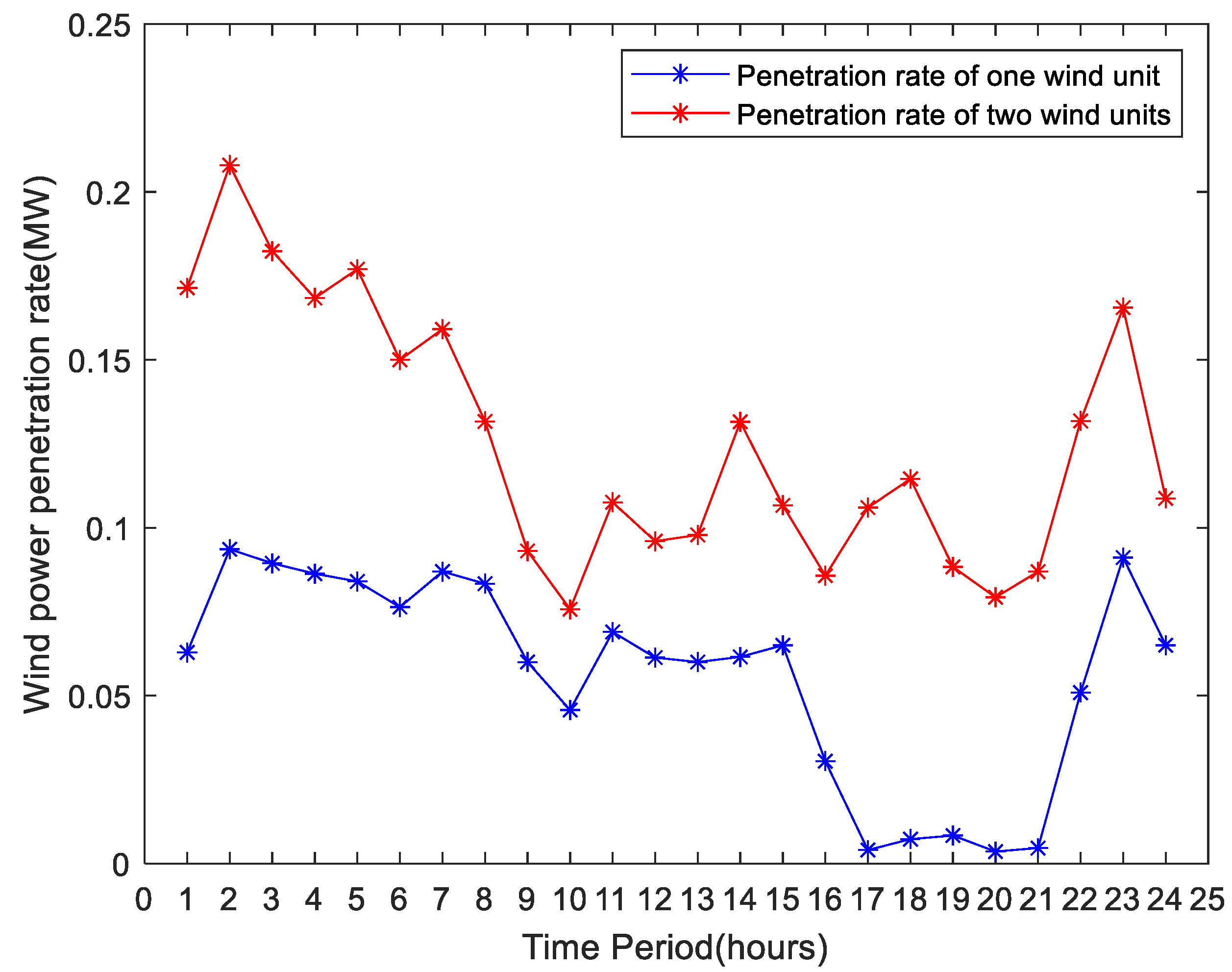
5. Maximum Penetration Rate of Wind Power Analysis and Discussion of Practical Implementation

In order to ensure the safe and stable operation of a power system after wind power integration, it is necessary to study the penetration rate of wind power, which is the percentage of wind power relative to the regional grid power. The wind power penetration rates of a system with one wind unit and two wind units at different time periods are shown in Figure 5. As shown in the figure, the wind power penetration rates of a system with two wind units are much higher than those of a system with one wind unit, and the maximum wind power penetration level of a system with two wind units exceeds 20%. Despite the higher the wind power penetration rate, the lower the total cost, the more challenges faced by a power system with high penetration of wind power, owing to the high volatility and intermittency of wind power. Therefore, curtailing of wind has to be considered to ensure secure operation of the system in some circumstances from the total cost point of view.

Based on the analysis presented above, it can be seen that for the stochastic UC problem with wind power, the CCP model considered in this paper is relatively simple; the average wind power permeability within 24 h is lower than 20%. In order to improve wind power utilization and ensure the safe operation of a power system, as suggested in [35,36], other energy sources and energy storage solutions can be combined to construct a more practical CCP model. However, the MISOCP derived in this paper is still a valid reformulation for the relevant CCP model.

6. Conclusions

Herein, we proposed a CCP model for the related UC problem that considers stochastic wind power and pollutant emission costs of thermal units. Chance constraints were introduced to describe the uncertainty output of wind power, and the system constraints were guaranteed by the satisfied probability. The CCP model was transformed into a deterministic equivalent form by Latin hypercube sampling and the K-means clustering algorithm, as well as the SAA method. A better formulation, MISOCP, was derived, which is based on the convex hull theory and can be effectively solved using the correct software. Numerical test results illustrate that the method presented in this paper is effective and suitable for solving the large-scale uncertain UC problem. However, the CCP model proposed in this paper is relatively simple, and an actual model closer to real-life scenarios will be constructed in future research.

References

1. Carrion, M.; Arroyo, J.M. A computationally efficient mixed-integer linear formulation for the thermal unit commitment problem. IEEE Trans. Power Syst. 2006, 21, 1371–1378. [Google Scholar] [CrossRef]
2. Morales-Espana, G.; Latorre, J.M.; Ramos, A. Tight and compact MILP formulation for the thermal unit commitment problem. IEEE Trans. Power Syst. 2013, 28, 4897–4908. [Google Scholar] [CrossRef]
3. Yang, L.; Chen, S.; Dong, Z. Multiple-periods locally-facet-based MIP formulations for the unit commitment problem. IEEE Trans. Power Syst. 2022. [Google Scholar] [CrossRef]
4. Yang, L.; Li, W.; Xu, Y.; Zhang, C.; Chen, S. Two novel locally ideal three-period unit commitment formulations in power systems. Appl. Energy 2021, 284, 116081. [Google Scholar] [CrossRef]
5. Abdi, H. Profit-based unit commitment problem: A review of models, methods, challenges, and future directions. Renew. Sust. Energy Rev. 2021, 138, 110504. [Google Scholar] [CrossRef]
6. Li, X.; Zhai, Q.; Zhou, J.; Guan, X. A variable reduction method for large-scale unit commitment. IEEE Trans. Power Syst. 2020, 35, 261–272. [Google Scholar] [CrossRef]
7. Zhu, X.; Zhao, S.; Yang, Z.; Zhang, N.; Xu, X. A parallel meta-heuristic method for solving large scale unit commitment considering the integration of new energy sectors. Energy 2022, 238, 121829. [Google Scholar] [CrossRef]
8. Xiang, Y.; Zhang, X. Unit commitment using Lagrangian relaxation and particle swarm optimization. Int. J. Elec. Power 2014, 61, 510–522. [Google Scholar]
9. Han, D.; Jian, J.; Yang, L. Outer approximation and outer-inner approximation approaches for unit commitment problem. IEEE Trans. Power Syst. 2014, 29, 505–513. [Google Scholar] [CrossRef]
10. Zhu, F.; Zhong, P.; Xu, B.; Liu, W.; Li, J. Short-term stochastic optimization of a hy-dro-wind-photovoltaic hybrid system under multiple uncertainties. Energy Convers. Manag. 2020, 214, 112902. [Google Scholar] [CrossRef]
11. Vatanpour, M.; Yazdankhah, A.S. The impact of energy storage modeling in coordination with wind farm and thermal units on security and reliability in a stochastic unit commitment. Energy 2018, 162, 476–490. [Google Scholar] [CrossRef]
12. Shahbazitabar, M.; Abdi, H. A novel priority-based stochastic unit commitment considering re-newable energy sources and parking lot cooperation. Energy 2018, 161, 308–324. [Google Scholar] [CrossRef]
13. Zhou, B.; Ai, X.; Fang, J.; Yao, W.; Zuo, W.; Chen, Z.; Wen, J. Data-adaptive robust unit commit-ment in the hybrid AC/DC power system. Appl. Energy 2019, 254, 113784. [Google Scholar] [CrossRef]
14. Sun, Y.; Dong, J.; Ding, L. Optimal day-ahead wind-thermal unit commitment considering statisti-cal and predicted features of wind speeds. Energy Convers. Manage. 2017, 142, 347–356. [Google Scholar] [CrossRef]
15. Ning, C.; You, F. Data-driven adaptive robust unit commitment under wind power uncertainty: A bayesian nonparametric approach. IEEE Trans. Power Syst. 2019, 34, 2409–2418. [Google Scholar]
16. Guo, G.; Zephyr, L.; Morillo, J.; Wang, Z.; Anderson, C.L. Chance constrained unit commitment approximation under stochastic wind energy. Comput. Oper. Res. 2021, 134, 105398. [Google Scholar] [CrossRef]
17. Zhao, C.; Wang, Q.; Wang, J.; Guan, Y. Expected value and chance constrained stochastic unit commitment ensuring wind power utilization. IEEE Trans. Power Syst. 2014, 29, 2696–2705. [Google Scholar] [CrossRef]
18. Wu, Z.; Zeng, P.; Zhang, X.P.; Zhou, Q. A Solution to the chance-constrained two-stage stochastic program for unit commitment with wind energy integration. IEEE Trans. Power Syst. 2016, 31, 4185–4196. [Google Scholar] [CrossRef]
19. Yang, Y.; Wu, W.; Wang, B.; Li, M. Analytical reformulation for stochastic unit commitment con-sidering wind power uncertainty with Gaussian mixture model. IEEE Trans. Power Syst. 2020, 35, 2769–2782. [Google Scholar] [CrossRef]
20. Adam, L.; Branda, M. Nonlinear chance constrained croblems: Optimality conditions, regulariza-tion and solvers. J. Optim. Theory Appl. 2016, 170, 419–436. [Google Scholar] [CrossRef]
21. Küçükyavuz, S.; Jiang, R. Chance-constrained optimization under limited distributional infor-mation: A review of reformulations based on sampling and distributional robustness. Euro J. Comput. Optim. 2022, 10, 100030. [Google Scholar] [CrossRef]
22. Akturk, M.S.; Atamturk, A.; Gurel, S. A strong conic quadratic reformulation for machine-job as-signment with controllable processing times. Oper. Res. Lett. 2009, 37, 187–191. [Google Scholar] [CrossRef] [Green Version]
23. Gunluk, O.; Linderoth, J. Perspective Relaxation of Mixed Integer Nonlinear Programs with Indica-Tor Variables. In International Conference on Integer Programming and Combinatorial Optimization; Springer: Berlin, Heidelberg, 2008; pp. 1–16. [Google Scholar]
24. Wang, Q.; Guan, Y.; Wang, J. A chance-constrained two-stage stochastic program for unit commit-ment with uncertain wind power output. IEEE Trans. Power Syst. 2012, 27, 206–215. [Google Scholar] [CrossRef]
25. Wang, J.; Shahidehpour, M.; Li, Z. Security-constrained unit commitment with volatile wind power generation. IEEE Trans. Power Syst. 2008, 23, 1319–1327. [Google Scholar] [CrossRef]
26. Ongsakul, W.; Petcharaks, N. Unit commitment by enhanced adaptive Lagrangian relaxation. IEEE Trans. Power Syst. 2004, 19, 620–628. [Google Scholar] [CrossRef]
27. Pereira, F.B.; Paucar, V.L.; Saraiva, F.S. Power System Unit Commitment Incorporating Wind Energy and Battery Energy Storage. In Proceedings of the 2018 IEEE XXV International Conference on Electronics, Electrical Engineering and Computing (INTERCON), Lima, Peru, 8–10 August 2018; pp. 1–4. [Google Scholar]
28. Mosek ApS[EB/OL]. Available online: https://www.mosek.com/ (accessed on 30 September 2020).
29. MathWorks[EB/OL]. Available online: https://www.mathworks.com/ (accessed on 16 March 2018).
30. Afkousi-Paqaleh, M.; Rashidinejad, M.; Pourakbari-Kasmaei, M. An implementation of harmony search algorithm to unit commitment problem. Electr. Eng. 2010, 92, 215–225. [Google Scholar] [CrossRef]
31. de Oliveira, L.M.; Junior, I.C.S.; Abritta, R.; Oliveira, E.D.S.; Nascimento, P.H.M.; Honorio, L.D.M. A hybrid algorithm for the unit commitment problem with wind uncertainty. Electr. Eng. 2022, 104, 1093–1110. [Google Scholar] [CrossRef]
32. Ji, B.; Yuan, X.; Chen, Z.; Tian, H. Improved gravitational search algorithm for unit commitment considering uncertainty of wind power. Energy 2014, 67, 52–62. [Google Scholar] [CrossRef]
33. Kokare, M.B.; Tade, S.V. Application of Artificial Bee Colony Method for Unit Commitment. In Proceedings of the 2018 Fourth International Conference on Computing Communication Control and Automation (ICCUBEA), IEEE, Pune, India, 16–18 August 2018; pp. 1–6. [Google Scholar]
34. Reddy, S.; Panwar, L.; Panigrahi, B.; Kumar, R.; AlSumaiti, A.S. An Application of Binary Grey Wolf Optimizer (BGWO) Variants for Unit Commitment Problem. In Applied Nature-Inspired Computing: Algorithms and Case Studies; Springer: Berlin/Heidelberg, Germany, 2020; pp. 97–127. [Google Scholar]
35. Yang, H.; Liang, R.; Yuan, Y.; Chen, B.; Xiang, S.; Liu, J.; Zhao, H.; Ackom, E. Distributionally robust optimal dispatch in the power system with high penetration of wind power based on net load fluctuation data. Appl. Energy 2022, 313, 118813. [Google Scholar] [CrossRef]
36. Li, Y.; Wang, J.; Han, Y.; Zhao, Q.; Fang, X.; Cao, Z. Roubst and opportunistic scheduling of district integrated natural gas and power system with high wind power penetration considering demand flexibility and compressed air enerby storage. J. Clean. Prod. 2020, 256, 120456. [Google Scholar] [CrossRef]
Figure 1. Sample points generated by Monte Carlo simulation.
Mathematics 11 00346 g001
Figure 2. Sample points generated by the Latin hypercube method.
Mathematics 11 00346 g002
Figure 3. Specific wind power outputs for five types of scenarios.
Mathematics 11 00346 g003
Figure 4. General solution procedure.
Mathematics 11 00346 g004
Figure 5. Permeability of wind power at different time periods.
Mathematics 11 00346 g005