Implicit Finite-Difference Scheme for a Duffing Oscillator with a Derivative of Variable Fractional Order of the Riemann-Liouville Type

Abstract

The article considers an implicit finite-difference scheme for the Duffing equation with a derivative of a fractional variable order of the Riemann–Liouville type. The issues of stability and convergence of an implicit finite-difference scheme are considered. Test examples are given to substantiate the theoretical results. Using the Runge rule, the results of the implicit scheme are compared with the results of the explicit scheme. Phase trajectories and oscillograms for a Duffing oscillator with a fractional derivative of variable order of the Riemann–Liouville type are constructed, chaotic modes are detected using the spectrum of maximum Lyapunov exponents and Poincare sections. Q-factor surfaces, amplitude-frequency and phase-frequency characteristics are constructed for the study of forced oscillations. The results of the study showed that the implicit finite-difference scheme shows more accurate results than the explicit one.

1. Introduction

The Duffing oscillator with a fractional derivative in the dissipative term is of great importance in solving applied problems of mathematics [1], physics [2,3,4] and chaos theory [5,6]. Fractional derivatives and their properties are presented in detail in the monograph [7]. The Duffing equation describes nonlinear oscillatory processes characterized by bistability and the presence of chaotic dynamics. In world practice, the bistability of nonlinear oscillations is of particular interest in optical technologies [8], power grids, etc. Identification of chaotic regimes is one of the main tasks, for example, in clinical medicine [9]. There are many methods for solving the fractional Duffing equation. The authors of [10] considered the method of homotopy analysis and the method of finite-difference schemes [5]; article [11] used a modified method of fractional power series. A qualitative analysis of the fractional Duffing oscillator can be found in articles [12,13,14,15,16,17,18,19,20,21,22,23,24,25,26,27,28,29]. However, they considered the case when the fractional derivative had a constant order.

The introduction of a fractional derivative of variable order into the Duffing equation will make it even more flexible to describe nonlinear oscillations with memory effects and chaotic modes. You can learn about equations of fractional variable order from the article [30]. The solution of the Duffing equation with a fractional variable order derivative can be found using numerical methods [31,32,33,34]. In particular, In particular, an explicit finite difference scheme was proposed in [35], and the Adams-Bashford-Moulton method was applied in Ref. [36]. There are many methods for studying chaotic and regular modes of fractional oscillators, for example, the selection of a suitable Lyapunov function [12], stabilization of the chaotic dynamics of the rational Zeraulia–Sprott mapping and the Ikeda mapping [13]. In [37], chaotic and regular modes are investigated using the spectrum of maximum Lyapunov exponents and Poincare sections. The stability of systems containing fractional derivatives of variable order of the Caputo type was considered in Ref. [38] on the example of discrete neural networks. Stability was considered according to Ulam–Hiers. For an explicit scheme, the issues of stability and convergence of [39] are theoretically justified. In the works [40,41], the properties of forced oscillations of a Duffing oscillator with a fractional derivative of variable order of the Riemann–Liouville type are investigated using amplitude-frequency (AFC), phase-frequency characteristics (PFC) and Q-factor. It turned out that the order of the fractional derivative affects the rate of attenuation of oscillations.

However, the accuracy of calculations according to the explicit scheme is not high. To improve the accuracy of calculations and reduce the error, an implicit finite-difference scheme is used in this work. Moreover, unlike the explicit scheme, the stability and convergence of the implicit one does not depend on the constraints on the step of the dishonest grid. In this article, by analogy with the works [35,37,39,40,41], an implicit finite-difference scheme for solving the Duffing equation with a fractional derivative of variable order of the Riemann–Liouville type is investigated, the issues of stability and convergence of the numerical scheme are substantiated, and chaotic regimes and bistability of oscillations are investigated.

The outline of the article has the following structure. Section 1 provides some background information about the subject of research. Section 2 gives the problem statement. Section 3 presents a numerical algorithm for solving the problem. The issues of convergence and stability of an implicit finite-difference scheme are investigated. Section 4 gives test examples of the operation of the numerical algorithm and its comparison with the explicit finite difference scheme. Using an implicit finite-difference scheme, chaotic and regular modes of the Duffing oscillator with a fractional derivative of variable order are studied. In Section 5, the forced oscillations of the fractional Duffing oscillator are studied. The amplitude-frequency and phase-frequency characteristics are built, as well as the quality factor of the oscillatory system. In Section 6, a conclusion is given on the results of the research.

2. Problem Statemant

Consider the following Cauchy problem for a nonlinear oscillation equation by analogy with the work of [39]:

$$\ddot{x}\left(t\right)+\lambda {\Theta }^{q\left(t\right)-1}{D}_{0t}^{q\left(t\right)}x\left(t\right)+{\omega }_{0}x\left(t\right)+f\left(x,t\right)=0,x\left(0\right)=x_0,\dot{x}\left(0\right)=y_0,$$

(1)

where $x\left(t\right)\in C^2\left(0,T\right)$ is the displacement function, $\lambda$ is the coefficient of viscous friction, ${\omega }_0$ is the natural frequency, $x_0,y_0$ are set constants that define the initial conditions, and $\Theta$ is the parameter responsible for the time scale. In Equation (1), the fractional derivative operator is taken in the sense of Riemann–Liouville.

Definition 1. 

Fractional Riemann–Liouville derivative of variable order $0<q\left(t\right)<1$ of the function $x\left(t\right)\in C^1[0,T],T>0$ has the form:

$$D_{0t}^{q\left(t\right)}x\left(t\right)=\frac{1}{\Gamma \left(1-q\left(t\right)\right)}\frac{d}{dt}\underset{0}{\overset{t}{\int }}\frac{x\left(\tau \right)d\tau }{{\left(t-\tau \right)}^{q\left(t\right)}},$$

(2)

where $\Gamma \left(y+1\right)=\underset{0}{\overset{\propto }{\int }}{x}^y{e}^{-x}dx$ is Euler’s gamma function.

The nonlinear function $f(x,t)$ satisfies the Lipschitz condition with respect to x:

$$\parallel f(x_1\left(t\right),t)-f(x_2\left(t\right),t)\parallel <L\parallel x_1\left(t\right)-x_2\left(t\right)\parallel ,$$

(3)

where $L>0$ is the Lipschitz constant.

Remark 1. 

Cauchy problem (1) is a mathematical model describing a wide class of nonlinear fractional oscillators, the type and type of which is determined by the function $f(x,t)$. The first term describes inertia force, the second term is friction force (damping) and the third is returning force of the oscillator.

Remark 2. 

If in Equation (1) $f(x,t)=b{x}^3-\delta cos\left(\omega t\right)$, where b is the nonlinearity coefficient, δ and ω are the amplitude and frequency of the external force, then we obtain the Duffing oscillator equation with a fractional derivative of variable order [39]. Later in Equation (1), we will assume $\Theta =1$.

Remark 3. 

It should be noted that the existence and uniqueness of systems similar to (1) were considered in [42].

3. Numerical Algorithm

Since Equation (1) is nonlinear, its solution is sought using finite difference schemes. We introduce a uniform computational grid. The segment $[0,T]$ will be divided into N equal parts in increments $h=\frac{T}{N}:0=t_0<t_1=h<t_2=2h<\dots <t_k=kh<\dots <t_N=T$. The functions $q\left(t\right),x\left(t\right),f\left(x\right(t),t)$ will go into the grid $q_k=q\left(t_k\right),x_k=x\left(t_k\right),f_k=f(x\left(t_k\right),t_k)$. Approximation of the second derivative gives:

$$\ddot{x}\left(t\right)=\frac{x_{k+1}-2x_k+x_{k-1}}{h^2}+O\left(h^2\right),$$

(4)

The fractional derivative of variable order is approximated by the Grunwald–Letnikov operator (5).

Definition 2. 

The fractional Grunwald-Letnikov derivative of variable order $0<q_k<1$ has the form:

$$\begin{array}{c}{\Delta }_{0k+1}^{q_{k+1}}{x}_{k+1}=\frac{1}{h^{q_{k+1}}}{\displaystyle \sum _{i=0}^{k+1}}{c}_i^{q_{k+1}}{x}_{k-i+1}+O\left(h\right),\hfill \\ c_i^{q_{k+1}}=\left(1-\frac{1+q_{k+1}}{i}\right)c_{i-1}^{q_{k+1}},c_0^{q_{k+1}}=1.\hfill \end{array}$$

(5)

Here, $c_i^{q_k}$ are the Grunwald–Letnikov weight coefficients. In [39], the following Lemma for weight coefficients was proved.

Lemma 1. 

The weighting coefficients $c_i^{q_k}$ have the following properties:

$$\begin{array}{c}{c}_0^{q_k}=1,c_1^{q_k}=-q_k,c_i^{q_k}<0(i\ne 1)\hfill \\ {\displaystyle \sum _{i=0}^{\infty }}{c}_i^{q_k}=0,\forall l=1,2,\dots ,{\displaystyle \sum _{i=1}^l}{c}_i^{q_k}<0\hfill \end{array}.$$

(6)

In [39], to solve the Cauchy problem (1), a non-local explicit finite difference scheme (EFDS) was constructed for $k=1,2,\dots ,N-1$:

$$x_{k+1}=A_k{x}_k-x_{k-1}-B_k\sum _{i=1}^k{c}_i^{q_k}{x}_{k-i}-h^2{f}_k,$$

(7)

where $A_k=2-\lambda h^{2-q_k}-h^2{\omega }_0,B_k=\lambda h^{2-q_k}$. The following theorems were also proved in Ref. [39]

Theorem 1. 

The explicit scheme (7) is stable if the condition $\lambda h^{2-Q}+h^2{\omega }_0^2\le 1$ is met.

Theorem 2. 

The explicit scheme (7) converges to an exact first-order solution if the condition $\lambda h^{2-Q}+h^2{\omega }_0^2\le 1$ is met.

In Theorems 1 and 2, $Q=\underset{k}{max}\left(q_k\right)$.

In this article, taking into account the relations (4) and (5), we construct a non-local implicit finite difference scheme (IFDS) and consider the issues of its stability and convergence. Let us make an implicit scheme. To do this, we substitute Formulas (4) and (5) into the Cauchy problem (1); as a result, we obtain the following difference equation:

$\begin{array}{l}\hspace{1em}\hspace{1em}\frac{x_{k+1}-2x_k+x_{k-1}}{h^2}+\frac{\lambda }{h^{q_{k+1}}}{\displaystyle \sum _{j=0}^{k+1}}{c}_j^{q_{k+1}}{x}_{k-j+1}+{\omega }_0^2{x}_{k+1}+f_{k+1}=\\ =x_{k+1}-2x_k+x_{k-1}+\frac{\lambda h^2}{h^{q_{k+1}}}{\displaystyle \sum _{j=0}^{k+1}}{c}_j^{q_{k+1}}{x}_{k-j+1}+h^2{\omega }_0^2{x}_{k+1}+h^2{f}_{k+1}=\\ =x_{k+1}-2x_k+x_{k-1}+\lambda h^{2-q_{k+1}}{\displaystyle \sum _{j=0}^{k+1}}{c}_j^{q_{k+1}}{x}_{k-j+1}+h^2{\omega }_0^2{x}_{k+1}+h^2{f}_{k+1}=\\ =x_{k+1}+h^2{\omega }_0^2{x}_{k+1}-2x_k+x_{k-1}+\lambda h^{2-q_{k+1}}{\displaystyle \sum _{j=0}^{k+1}}{c}_j^{q_{k+1}}{x}_{k-j+1}+h^2{f}_{k+1}=\\ =(1+h^2{\omega }_0^2)x_{k+1}-2x_k+x_{k-1}+\lambda h^{2-q_{k+1}}{\displaystyle \sum _{j=0}^{k+1}}{c}_j^{q_{k+1}}{x}_{k-j+1}+h^2{f}_{k+1}=0.\end{array}$

As a result, we obtain the following implicit finite-difference scheme:

$$(1+h^2{\omega }_0)x_{k+1}-2x_k+x_{k-1}+B_{k+1}\sum _{i=0}^{k+1}{c}_i^{q_{k+1}}{x}_{k-i+1}-h^2{f}_{k+1}=0,$$

(8)

where $B_{k+1}=\lambda h^{2-q_{k+1}}$.

Remark 4. 

EFDS (7) approximates the differential problem (1) in the inner nodes of the grid with the second order. However, due to the approximation of the second initial condition in (1) $\dot{x}\left(0\right)=\frac{x_1-a}{h}+O\left(h\right)$, the global approximation order is reduced to the first.

Remark 5. 

To construct a finite difference scheme, the displacement function must be considered in the third class of smooth functions $x\left(t\right)\in C^3\left[0,T\right]$.

Stability and convergence of IFDS

Definition 3. 

The difference approximation (8) is stable if for any error vector between the exact and numerical solution $E_0$ there is a positive number $Q_k:\underset{k\to \infty }{lim}{Q}_k=0$ and the condition is met [39]:

$$∥E_{k+1}∥\le Q_k∥E_0∥.$$

(9)

Theorem 3. 

The implicit finite-difference scheme (8) is certainly stable.

Proof of Theorem 3. 

Let the error be ${\epsilon }_k={\overline{x}}_k-x_k,k=0,\dots ,N$, where ${\overline{x}}_k$ is the approximate solution of the Cauchy problem (1). Then, Equation (8) in terms of error will take the form:

$$\begin{array}{c}\left(1+h^2{\omega }_0^2\right){\epsilon }_{k+1}=2{\epsilon }_k-{\epsilon }_{k-1}-B_{k+1}\sum _{j=0}^{k+1}{c}_j^{q_{k+1}}{\epsilon }_{k-j+1}-\hfill \\ \hfill -h^2\left(f\left({\overline{x}}_{k+1},t_{k+1}\right)-f\left(x_{k+1},t_{k+1}\right)\right),k=1,\dots ,N-1.\end{array}$$

(10)

Let us introduce the norm ${∥E_{k+1}∥}_{\infty }={\displaystyle \underset{k}{max}}\left|{\epsilon }_{k+1}\right|$. Proceeding to (10) for the absolute value, we obtain:

$$\left(1+h^2{\omega }_0^2\right)\left|{\epsilon }_{k+1}\right|\le 2\left|{\epsilon }_k\right|-\left|{\epsilon }_{k-1}\right|-B_{k+1}\sum _{j=0}^{k+1}{c}_j^{q_{k+1}}\left|{\epsilon }_{k-j+1}\right|-$$

$$-h^2\left(\left|f\left({\overline{x}}_{k+1},t_{k+1}\right)-f\left(x_{k+1},t_{k+1}\right)\right|\right)\le \left|{\epsilon }_k\right|-B_{k+1}\sum _{j=0}^{k+1}{c}_j^{q_{k+1}}\left|{\epsilon }_{k-j+1}\right|-h^{2}L\left|{\epsilon }_{k+1}\right|$$

Let us move on to the norm. By virtue of Lemma 1, Lipschitz conditions (3) and $L>0$, we obtain the estimate

$$\left(1+h^2{\omega }_0^2+h^{2}L\right){∥E_{k+1}∥}_{\infty }\le {∥E_k∥}_{\infty }-B_{k+1}\sum _{j=0}^{k+1}{c}_j^{q_{k+1}}{∥E_{k-j+1}∥}_{\infty }\le {∥E_k∥}_{\infty }$$

$${∥E_{k+1}∥}_{\infty }\le \frac{1}{\left(1+h^2{\omega }_0^2+h^{2}L\right)}{∥E_k∥}_{\infty }\le \frac{1}{{\left(1+h^2{\omega }_0^2+h^{2}L\right)}^k}{∥E_0∥}_{\infty }.$$

i.e., with $k\to \infty ,{∥E_{k+1}∥}_{\infty }\to 0$. The theorem is proved. □

Let $x\left(t_k\right)$ be the exact solution of the Cauchy problem (1) at the point $t_k$. Define ${\eta }_k=x\left(t_k\right)-x_k$ and accordingly the vector $Y_k={\left({\eta }_1,\dots ,{eta}_k\right)}^T$. Note that $Y_0$ is a null vector. Substituting $x_k=x\left(t_k\right)-{\eta }_k$ into Equation (8), we obtain:

$$\begin{array}{c}\left(1+h^2{\omega }_0^2\right){\eta }_{k+1}=2{\eta }_k-{\eta }_{k-1}-B_{k+1}\sum _{j=0}^{k+1}{c}_j^{q_{k+1}}{\eta }_{k-j+1}-\hfill \\ \hfill -h^2\left(f\left(x\left(t_{k+1}\right),t_{k+1}\right)-f\left(x_{k+1},t_{k+1}\right)\right)+h^2{R}_{k+1}.\end{array}$$

(11)

Here,

$$\left|R_{k+1}\right|\le Ch,$$

where C is a constant independent of the step h of the calculated grid. The following theorem is valid.

Theorem 4. 

The implicit finite-difference scheme (8) certainly converges to the exact solution with the first order.

Proof of Theorem 4. 

Let us go to (11) for the absolute value, where we obtain:

$$\left(1+h^2{\omega }_0^2\right)\left|{\eta }_{k+1}\right|\le 2\left|{\eta }_k\right|-\left|{\eta }_{k-1}\right|-B_{k+1}\sum _{j=0}^{k+!}{c}_j^{q_{k+1}}\left|{\eta }_{k-j+1}\right|-$$

$$-h^2\left(\left|f\left(x\left(t_{k+1}\right),t_{k+1}\right)-f\left(x_{k+1},t_{k+1}\right)\right|\right)+$$

$$+h^{2}Ch\le 2\left|{\eta }_k\right|-\left|{\eta }_{k-1}\right|-B_{k+1}\sum _{j=0}^{k+1}{c}_j^{q_{k+1}}\left|{\eta }_{k-j+1}\right|-h^{2}L\left|{\eta }_{k+1}\right|+C{h}^3.$$

$$\left(1+h^2{\omega }_0^2\right){∥Y_{k+1}∥}_{\infty }\le {∥Y_k∥}_{\infty }-B_{k+1}\sum _{j=0}^{k+1}{c}_j^{q_{k+1}}{∥Y_{k-j+1}∥}_{\infty }-h^{2}L{∥Y_{k+1}∥}_{\infty }+C{h}^3.$$

Let us move on to the norm. By virtue of Lemma 1, Lipschitz conditions (3) and $L>0$, we obtain the estimate

$${∥Y_{k+1}∥}_{\infty }\le \frac{1}{\left(1+h^2{\omega }_0^2+h^{2}L\right)}{∥Y_k∥}_{\infty }+Ch\le \frac{1}{{\left(1+h^2{\omega }_0^2+h^{2}L\right)}^k}{∥Y_0∥}_{\infty }+$$

$$+\left(\frac{1}{{\left(1+h^2{\omega }_0^2+h^{2}L\right)}^k}+\frac{1}{{\left(1+h^2{\omega }_0^2+h^{2}L\right)}^{k-1}}+\dots +1\right)Ch,$$

i.e., with $k\to \infty ,{∥Y_{k+1}∥}_{\infty }\to Ch$. The theorem is proved. □

4. Numerical Examples

To confirm the theoretical results, let us consider some test examples. Let the nonlinear function in the model Equation (1) have the form $f(x,t)=b{x}^3\left(t\right)-b{t}^9-{\omega }_0{t}^3-6t-\lambda {\displaystyle \frac{d}{dt}}\left({\displaystyle \frac{\Gamma \left(4\right)t^{4-q\left(t\right)}}{\Gamma (5-q(t\left)\right)}}\right)$. Then the exact solution of the new Cauchy problem is in the form:

$$x\left(t\right)=t^3.$$

(12)

The error of the NCRS (8) is found with the formula:

$$\epsilon =max\left(|x_M^{ex}\left[j\right]-x_M\left[j\right]|\right),j=0,\dots ,N,$$

(13)

where $x_M^{ex}\left[j\right]$ is the exact solution (12), $x_M\left[j\right]$ is the numerical solution obtained by the scheme (8). If the exact solution is unknown, then we use the Runge rule:

$$\epsilon =max\left(|x_{2j}-x_j|\right),j=0,\dots ,N,$$

(14)

where $x_{2j}$ is the numerical solution at step h, $x_j$ is the numerical solution at step $h/2$.

The computational accuracy (8) is determined by the formula:

$$\alpha =\frac{ln\left(\frac{|{\epsilon }_i|}{|{\epsilon }_{i+1}|}\right)}{ln\left(2\right)},$$

(15)

where ${\epsilon }_i$ is an error at step $h/2^i$, ${\epsilon }_{i+1}$ is an error at step $h/2^{i+1}$, $i=0,1,\dots ,M-1$.

Let us compare the results obtained with the help of the EFDS (7) and the IFDS (8).

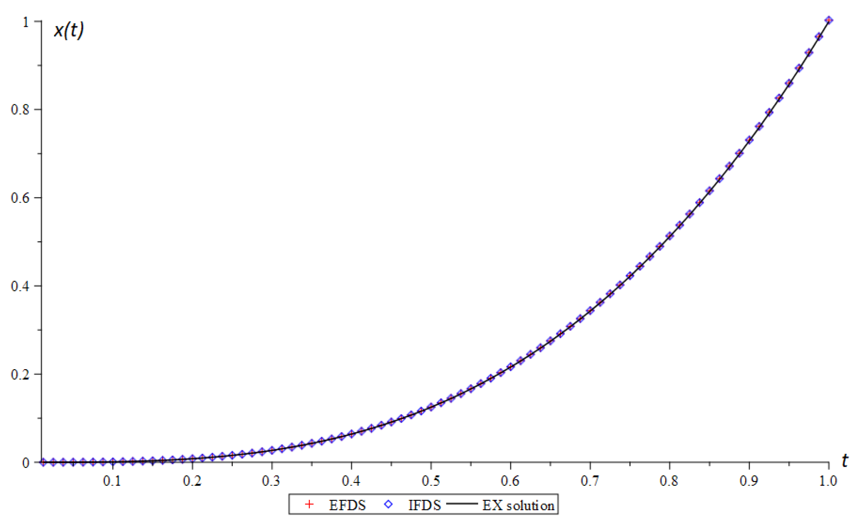
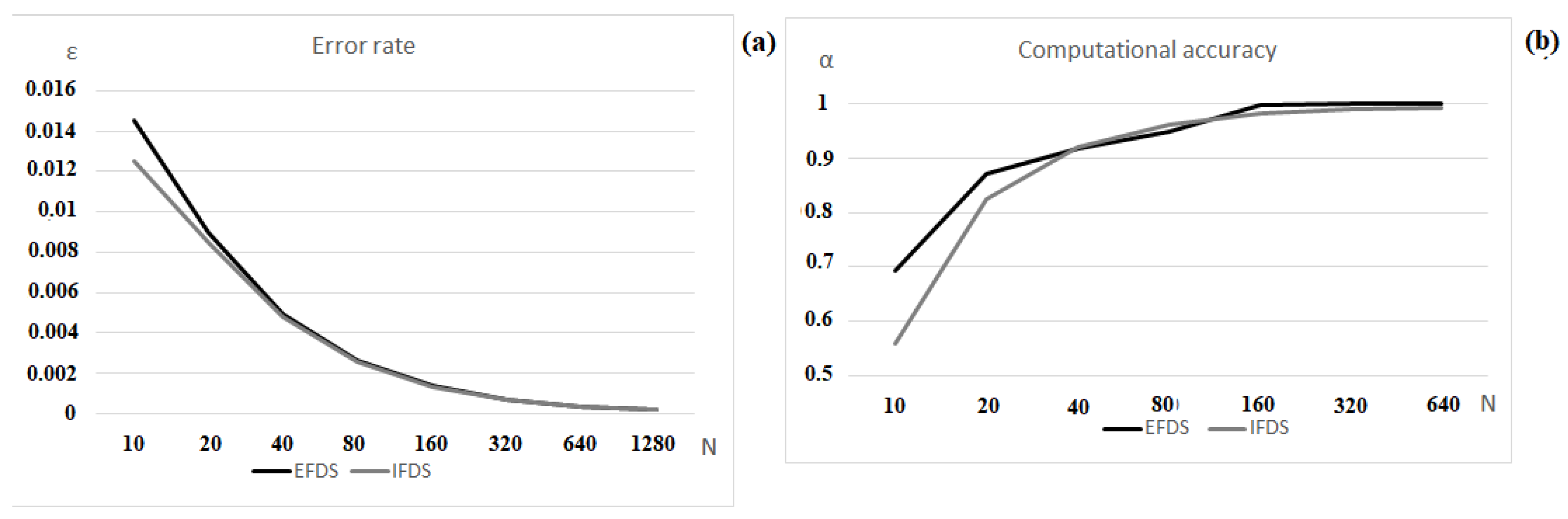
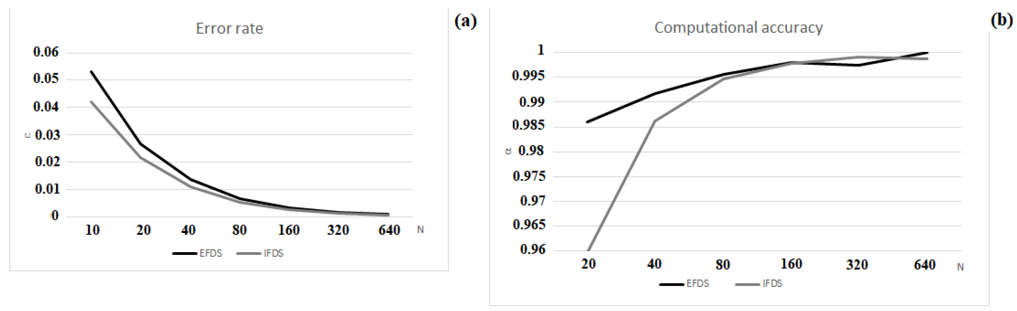
Example 1. 

Let us consider the case when the conditions of Theorems 1 and 2 are met for the EFDS. In the model Equation (1), we select the following parameters: $t\in [0,2],x\left(0\right)=\dot{x}\left(0\right)=0$, $\lambda =1$, ${\omega }_0=b=\delta =1,\omega =2,q\left(t\right)=0.8cos\left(0.5t\right),\lambda h^{2-Q}+h^2{\omega }_0^2=0.908$ and $Q=\underset{k}{max}\left(q\left(t_k\right)\right).$

According to Figure 1 and Figure 2, it can be seen that the EFDS and IFDS approximate the exact solution quite well (12). However, the error shown in Figure 2a for the IFDS is less than the error for the EFDS. This means that the IFDS (8) shows more accurate results than the EFDS (7). The computational accuracy (Figure 2b) for the EFDS and IFDS takes values close to 1 with increasing grid nodes, which indicates the first order of convergence of the EFDS (7) and IFDS (8) to the exact solution (12).

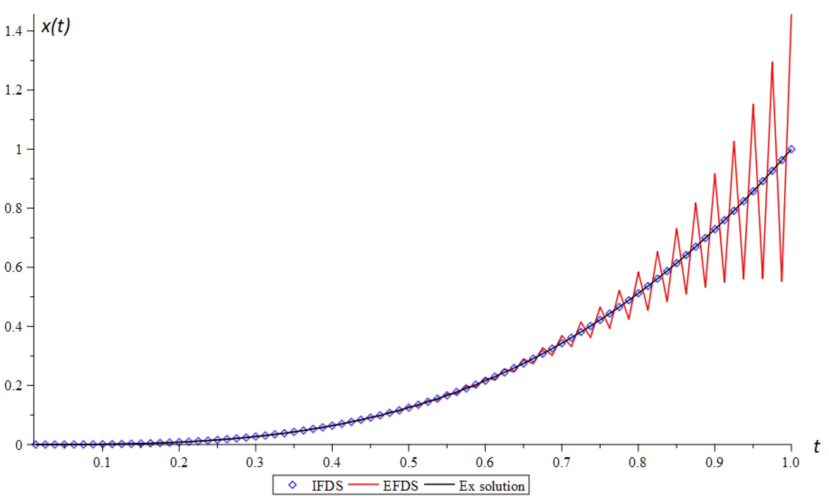
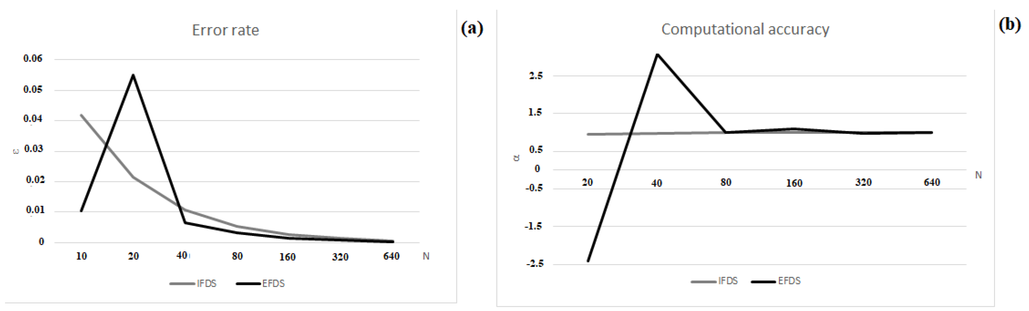
Example 2. 

Let us consider the case when the conditions of Theorems 1 and 2 are violated for the EFDS. In the model Equation (1), we select the following parameters: $t\in [0,2],x\left(0\right)=\dot{x}\left(0\right)=0,\lambda =3,{\omega }_0=10,b=\delta =1,\omega =2,q\left(t\right)=0.8cos\left(0.5t\right),\lambda h^{2-Q}+h^2{\omega }_0^2=1.2$ and $Q=\underset{k}{max}\left(q\left(t_k\right)\right).$

If conditions of Theorems 1 and 2 are violated, the anchor (7) diverges (Figure 3). At the same time, the IFDS (8) approximates the exact solution with a sufficiently high accuracy. According to Figure 4 and it can be seen that, in the interval of violation of the conditions of Theorems 1 and 2, the error and computational accuracy of EFDS change abruptly. For IFDS, the computational accuracy takes values close to 1. All these suggest that the stability and convergence of the IFDS (8) do not depend on step constraints and this confirms the validity of Theorems 3 and 4 on unconditional stability and convergence.

Let us compare the results of the EFDS (7) and the IFDS (8) for the fractional Duffing oscillator. The nonlinear function $f(x,t)$ is taken in the form presented in Remark 1. Since the Duffing oscillator does not have an exact solution, the error is calculated according to the Runge rule (14).

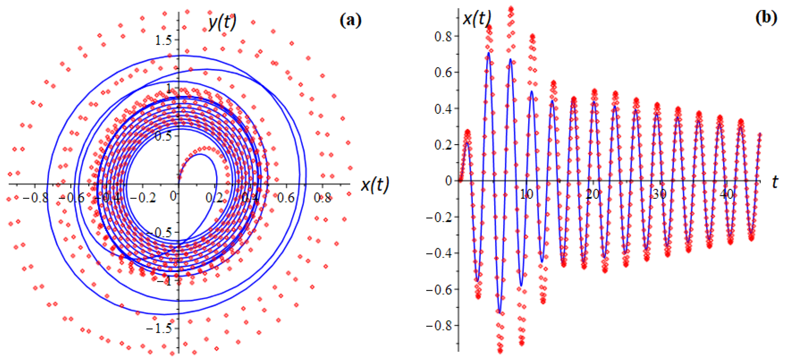
Example 3. 

In the model Equation (1), we select the following parameters: $t\in [0,50],x\left(0\right)=\dot{x}\left(0\right)=0,\lambda =1,{\omega }_0=b=\delta =1,\omega =2,q\left(t\right)=0.8cos\left(0.5t\right),\lambda h^{2-Q}+h^2{\omega }_0^2=0.9796$ and $Q=\underset{k}{max}\left(q\left(t_k\right)\right).$

The Duffing oscillator has various oscillatory regular and chaotic modes. Regular modes can be periodic. Figure 5 presents an example of two periodic modes. The waveform in Figure 5b shows that, over time, the oscillations reach a steady two-period regime, and the phase trajectory of Figure 5a has the form of two closed loops, which characterizes several periods of oscillation.

From Figure 6a,b we see that increasing the nodes of the computational grid by factor of 2 leads to a reduction in error by factor of 2, while the computational accuracy of the method tends to 1.

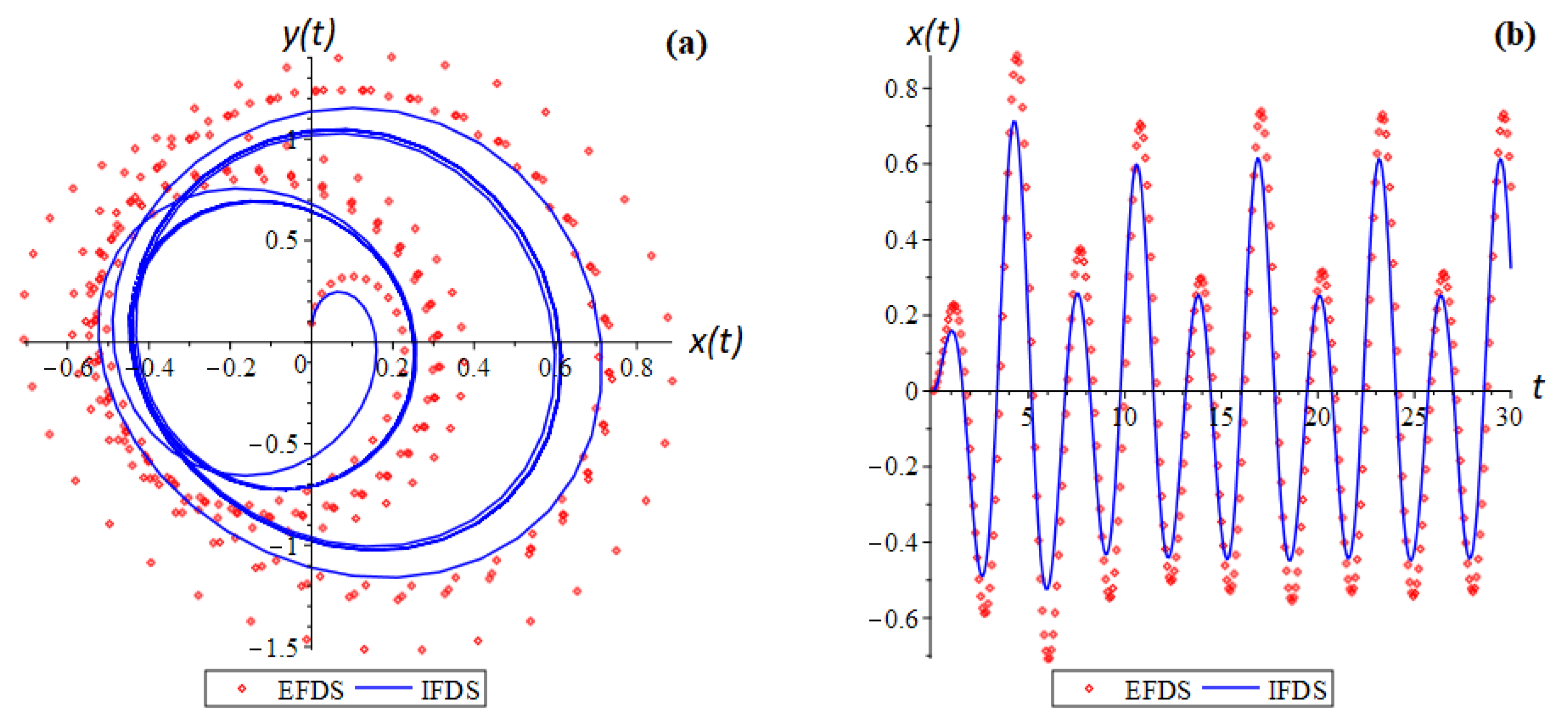
Example 4. 

Let us consider the case when the conditions of Theorems 1 and 2 are violated for the NCR. In the model Equation (1), we select the following parameters: $t\in [0,50],x\left(0\right)=\dot{x}\left(0\right)=0,\lambda =5,{\omega }_0=8,b=\delta =1,\omega =2,q\left(t\right)=0.8cos\left(0.5t\right),\lambda h^{2-Q}+h^2{\omega }_0^2=1.15$ and $Q=\underset{k}{max}\left(q\left(t_k\right)\right).$

In violation of the conditions of Theorems 1 and 2 for the EFDS, the error (Figure 7a) and computational accuracy (Figure 7b) of the method has a pronounced non-monotonic character in changing its values, which confirms the violation of the stability and convergence of scheme (7). The stability of the IFDS (8), in turn, does not depend on the conditions of Theorems 1 and 2.

Further in the article, the application of IFDS to the study of chaotic regimes, as well as forced oscillations of the fractional Duffing oscillator, are presented.

5. The Duffing Oscillator: Chaotic Mods and Forced Fluctuations

In the study of nonlinear systems, one of the important tasks is to determine the type of oscillations—periodic, quasi-periodic, random or chaotic [5]. A feature of chaotic oscillations is their high sensitivity to small changes in initial conditions. Therefore, one of the most reliable ways to detect chaos is to determine the rate of run-up of trajectories, which is estimated using the spectrum of Lyapunov exponents. The spectrum of maximum Lyapunov exponents was constructed using a modified Wolf–Bennetin algorithm [43], taking into account the Gram–Schmidt orthogonalization procedure, which was discussed in detail in [37], as well as with the use of an implicit scheme.

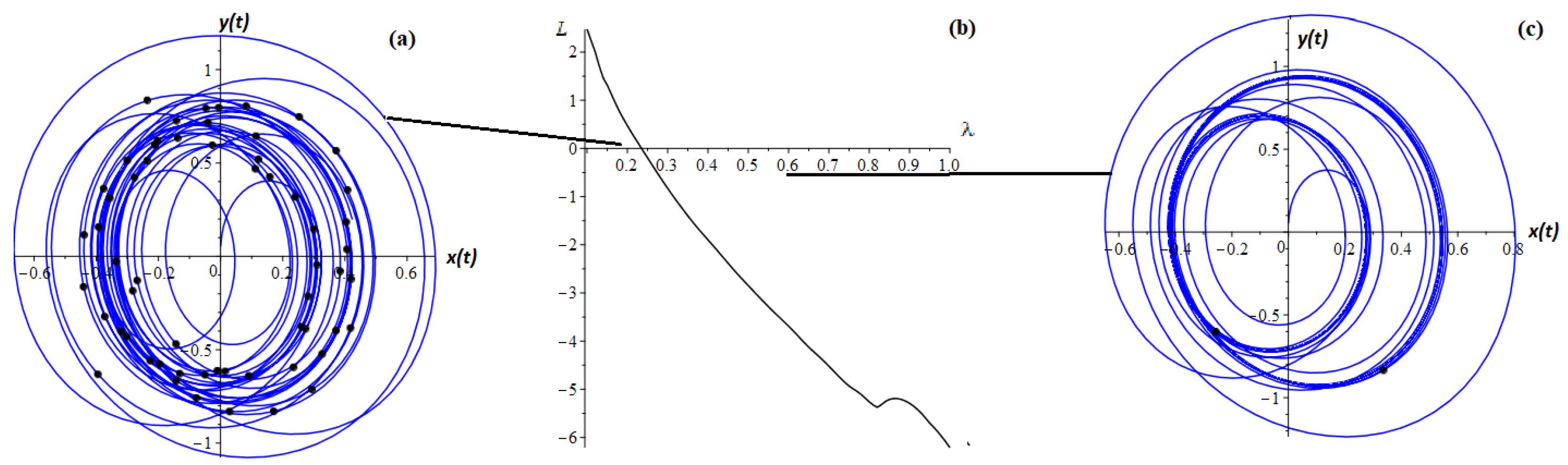
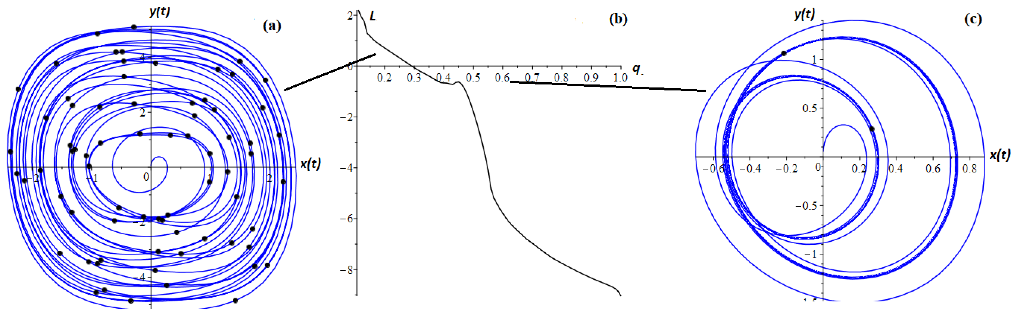
Remark 6. 

The presence of at least one positive Lyapunov exponent in the spectrum means the presence of a chaotic regime (asymptotic instability) of the considered phase trajectory [37]. A negative indicator indicates a regular regime.

Remark 7. 

Chaotic modes can be determined using Poincare sections. If the Poincare sections are a cloud, then a chaotic mode [5] is observed.

Example 5. 

In the problem (1), we select the following parameters: $q\left(t\right)=0.8{cos}^2\left(0.5t\right),t\in [0,50],x\left(0\right)=\dot{x}\left(0\right)=0,{\omega }_0=\delta =b=1$ and $\omega =2$.

Example 6. 

Let us choose the following parameters: $h=0.025,t\in [0,50],x\left(0\right)=\dot{x}\left(0\right)=0,\lambda ={\omega }_0=b=1,\omega =2$ and $\delta =1$.

Figure 8b and Figure 9b show the spectra of maximum Lyapunov exponents depending on $\lambda$ and q, respectively. With positive values of Lyapunov exponents, the phase trajectories enter a chaotic mode (Figure 8a and Figure 9a), and with negative values—a regular one (Figure 8c and Figure 9c).

Consider an example with other types of function $q\left(t\right)$.

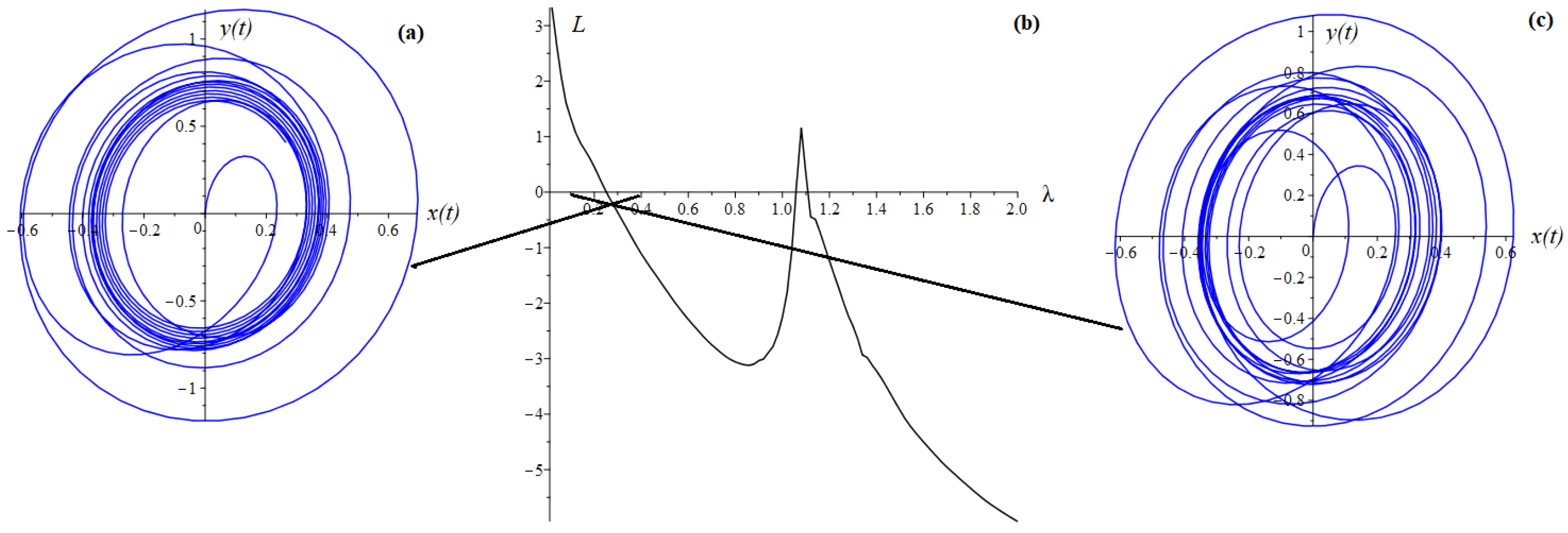
Example 7. 

In the model Equation (1), we select the following parameters: $t\in [0,T]$, $T=50$, $x\left(0\right)=\dot{x}\left(0\right)=0,\lambda =1,{\omega }_0=b=\delta =1,\omega =2,q\left(t\right)=0.1+\frac{1}{1.2T}t$ and $Q=\underset{k}{max}\left(q\left(t_k\right)\right).$

Example 7 shows that if the function $q\left(t\right)$ monotonically increases, then the oscillations decay (Figure 10b).

Figure 11 for Example 7 shows the bifurcation diagram and phase trajectories that correspond to different lambda values. It can be seen that the spectrum of maximum Lyapunov exponents contains positive values and, therefore, there is a chaotic regime.

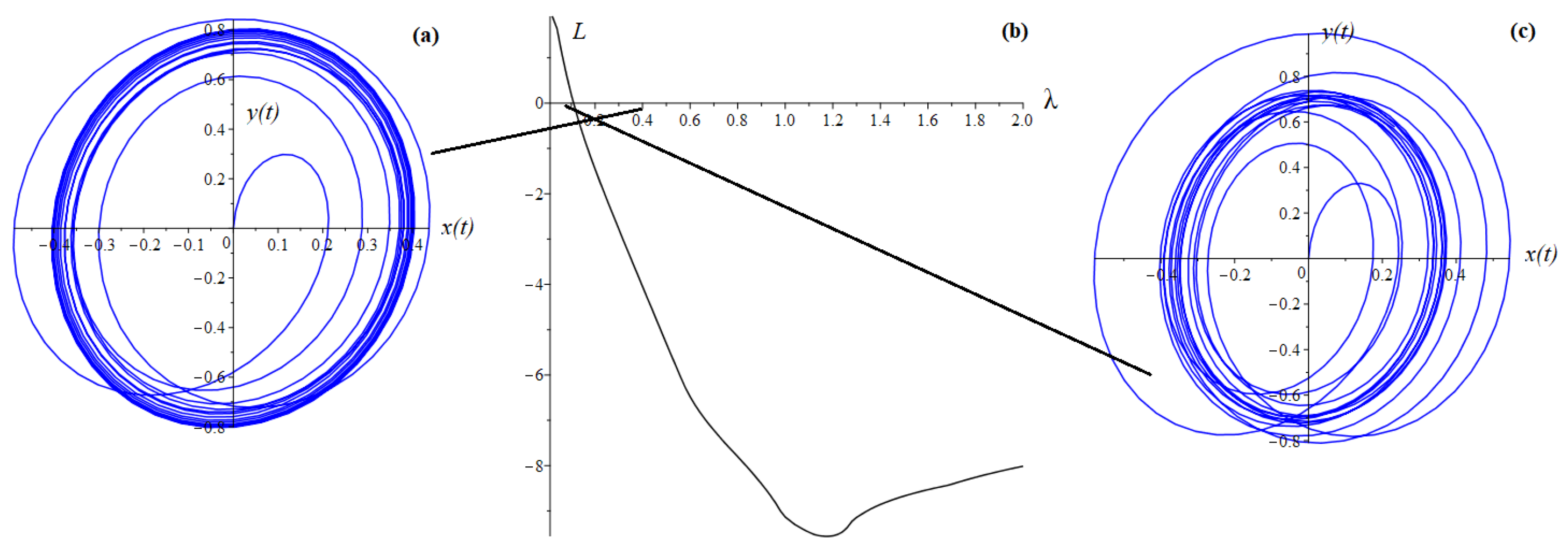
Example 8. 

In the model Equation (1), we select the following parameters: $t\in [0,T]$, $T=50$, $x\left(0\right)=\dot{x}\left(0\right)=0,\lambda =1,{\omega }_0=b=\delta =1,\omega =2,q\left(t\right)=0.96-\frac{1}{1.2T}t$ and $Q=\underset{k}{max}\left(q\left(t_k\right)\right).$

For Example 8, with a monotonically decreasing function $q\left(t\right)$, the oscillation amplitude begins to increase (Figure 12b). This is explained by the fact that the order of the fractional derivative is given in the dissipative term in the Cauchy problem (1) that defines viscous friction. With a decrease in the order of $q\left(t\right)$, the friction decreases, and the energy of the system increases, and with a decrease in the order, the energy costs of the system increase, respectively, the oscillations fade.

Figure 13 for Example 8 shows the bifurcation diagram and phase trajectories constructed for different values of the lambda parameters. Here we also see the presence of chaotic regimes.

Of great interest is the study of systems under the influence of various kinds of variable disturbing loads on them. Fluctuations in such systems caused by periodic external forces are called forced [40]. Different disturbing forces correspond to different scenarios of the behavior of the oscillatory system, which, thus, are no longer completely determined by the system’s own characteristics, but reflect its reaction to the disturbing force [44].

For practice, the most important cases are those when $f(x,t)$ contains a periodic function depending only on time t, which has its own frequency and amplitude, different from the system under consideration. In this case, there is a superposition of oscillations of the external periodic force and natural oscillations of the system. The oscillations described by Equation (1) will reach a certain steady state over time. In such systems, it is often possible to observe such phenomena as resonance and bistability [8,41]. To study these phenomena, one of the important tasks is the construction of amplitude-frequency (frequency response), phase-frequency characteristics (frequency response) and Q-factor.

Definition 4. 

AFC is the dependence of the amplitude of steady-state oscillations of the output signal of a certain system on the frequency of its input harmonic signal.

Definition 5. 

PFC is the dependence of the phase difference between the output and input signals on the frequency of the signal.

Definition 6. 

Q-factor is a quantitative characteristic of the resonant properties of oscillatory systems, showing how many times the total energy of the system is greater than the consumed.

In [40,41], the following theorem was proved using the harmonic balance method.

Theorem 5. 

The Cauchy problem (1) is equivalent to the linear Cauchy problem with integer derivative:

$$\ddot{x}\left(t\right)+p(\omega ,t)\dot{x}\left(t\right)+s^2(\omega ,t)x\left(t\right)=\delta cos\left(\omega t\right),x\left(0\right)=x_0,\dot{x}\left(0\right)=y_0,$$

(16)

In Equation (16), the coefficients $p(\omega ,t)$ and $s^2(\omega ,t)$ are searched as:

$$p(\omega ,t)=-2\lambda {\omega }^{q\left(t\right)-1}sin\left(\frac{q\left(t\right)\pi }{2}\right)+$$

$$2\lambda \frac{dq}{dt}{\omega }^{q\left(t\right)-2}\left[(ln\left(\omega \right)-\Psi (1-q\left(t\right)))cos\left(\frac{q\left(t\right)\pi }{2}\right)+\frac{\pi sin\left(\frac{q\left(t\right)\pi }{2}\right)}{2}\right],$$

(17)

$$s^2(\omega ,t)={\omega }_0^2-2\lambda {\omega }^{q\left(t\right)}cos\left(\frac{q\left(t\right)\pi }{2}\right)+\frac{3A^{2}b}{4}-$$

(18)

$$2\lambda \frac{dq}{dt}{\omega }^{q\left(t\right)-1}\left[(ln\left(\omega \right)-\Psi (1-q\left(t\right)))sin\left(\frac{q\left(t\right)\pi }{2}\right)+\frac{\pi cos\left(\frac{q\left(t\right)\pi }{2}\right)}{2}\right].$$

$\Psi (1-q\left(t\right))=-\gamma +{\displaystyle \sum _{n=1}^{\infty }}\left({\displaystyle \frac{1}{n}}-{\displaystyle \frac{1}{n+1-q\left(t\right)}}\right)$ is a digamma function, where $\gamma =\frac{1}{2}(\sqrt[3]{10}-1)$ is Euler’s constant.

For the linear Cauchy problem, formulas for calculating the frequency response, frequency response and Q-factor are known [41]:

$$A\left(\omega \right)=\frac{\delta }{\sqrt{{(s^2(\omega ,t)-{\omega }^2)}^2+p^2(\omega ,t){\omega }^2}},$$

(19)

$$\varphi \left(\omega \right)=arctan\left(\frac{p(\omega ,t)\omega }{(s^2(\omega ,t)-{\omega }^2)}\right),$$

(20)

$$Q=\frac{s(\omega ,t)}{p(\omega ,t)}.$$

(21)

We construct the frequency response and Q-factor surfaces for the nonmonotonic function $q\left(t\right)=0.8cos\left(0.5t\right)$ using Formulas (19)–(21).

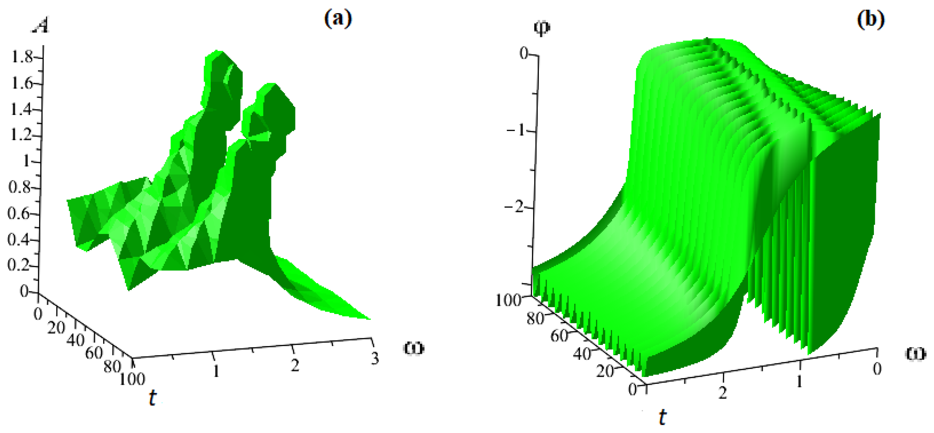
Example 9. 

In the model Equation (1), we choose the following parameters: $q\left(t\right)=0.8cos\left(0.5t\right)$, $t\in [0,100]$, $h=0.05,x\left(0\right)=\dot{x}\left(0\right)=0,\lambda =1,{\omega }_0=b=\delta =1,\omega \in [0,3]$ and $h_{\omega }=0.6$.

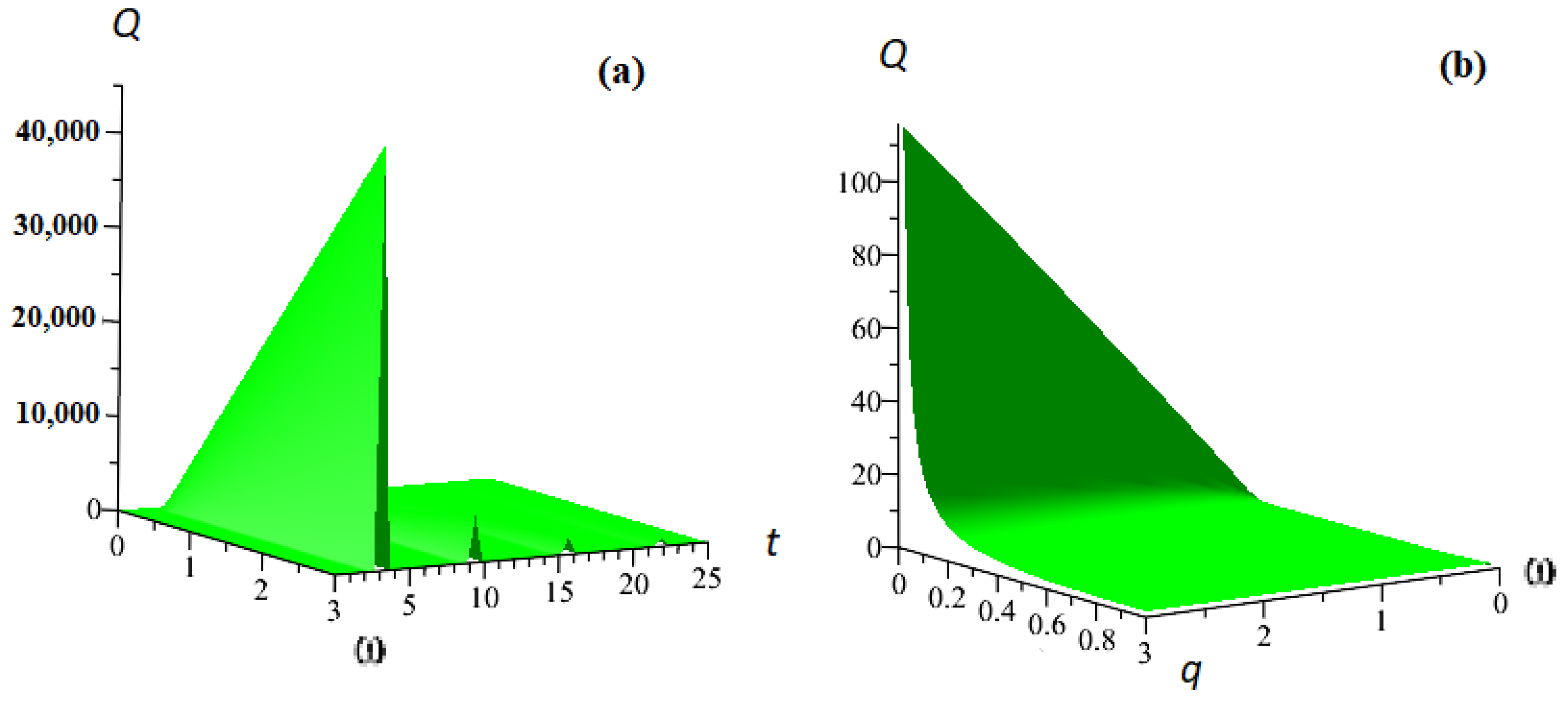
In Figure 14, the surfaces of AFC (Figure 14a) and PFC (Figure 14b) are given for the nonmonotonic function $q\left(t\right)$. In Figure 15, the Q-factor surface is given, taking into account the change in the exponent of the fractional derivative according to the law $q\left(t\right)=0.8cos\left(0.5t\right)$. Figure 15b shows the Q-factor surface when the parameter $q\in [0,1]$ is an independent variable. According to Figure 15b, it can be seen that when the parameter q decreases, the quality factor increases. The maximum amplitude corresponds to the maximum Q-factor, and when the frequency decreases, the Q-factor decreases. However, most of the quality factors depend on the parameter q.

Let us build AFC on the plane. To do this, we carry out the calculation according to schemes (7) and (8) with a sufficiently long simulation time, at which the forced oscillations reach a steady state. Next, the amplitude values are fixed at different values of the frequency of external influence, we obtain the dependence $A\left(\omega \right)$, which is plotted by points. Analytical frequency response will be constructed at a fixed time value corresponding to the maximum value of the amplitude of steady-state oscillations according to Formulas (19)–(21), i.e., for a constant value of the fractional derivative.

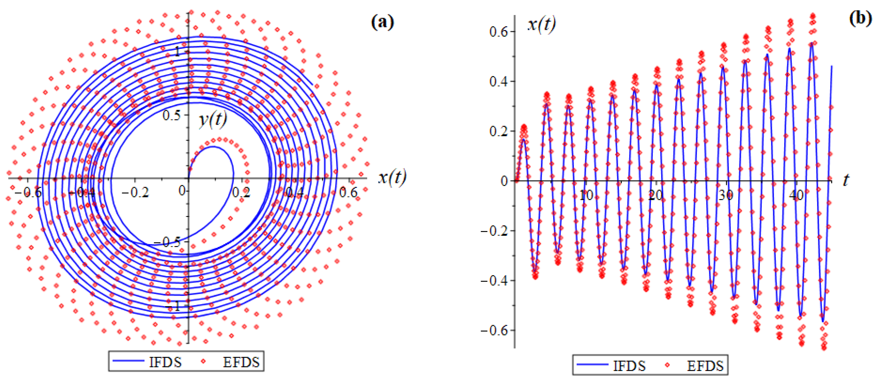
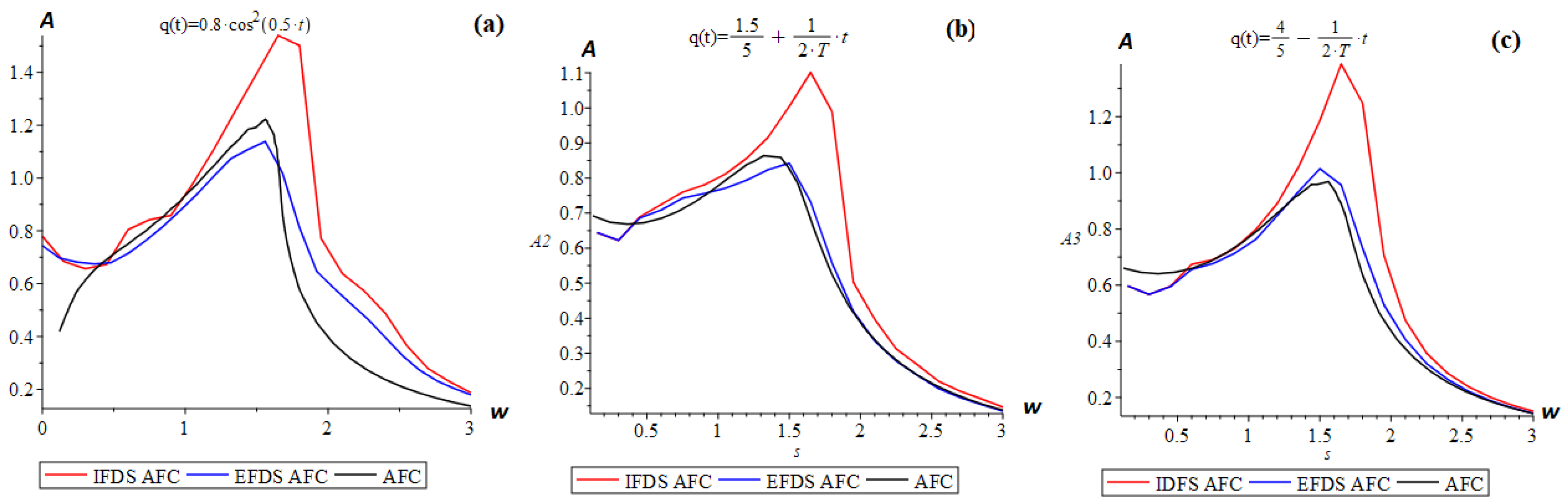
Example 10. 

In the model Equation (1), we select the following parameters: $t\in [0,100]$, $h=0.05$, $x\left(0\right)=\dot{x}\left(0\right)=0,\lambda =1,{\omega }_0=b=\delta =1,\omega \in [0,3]$ and $h_{\omega }=0.6$.

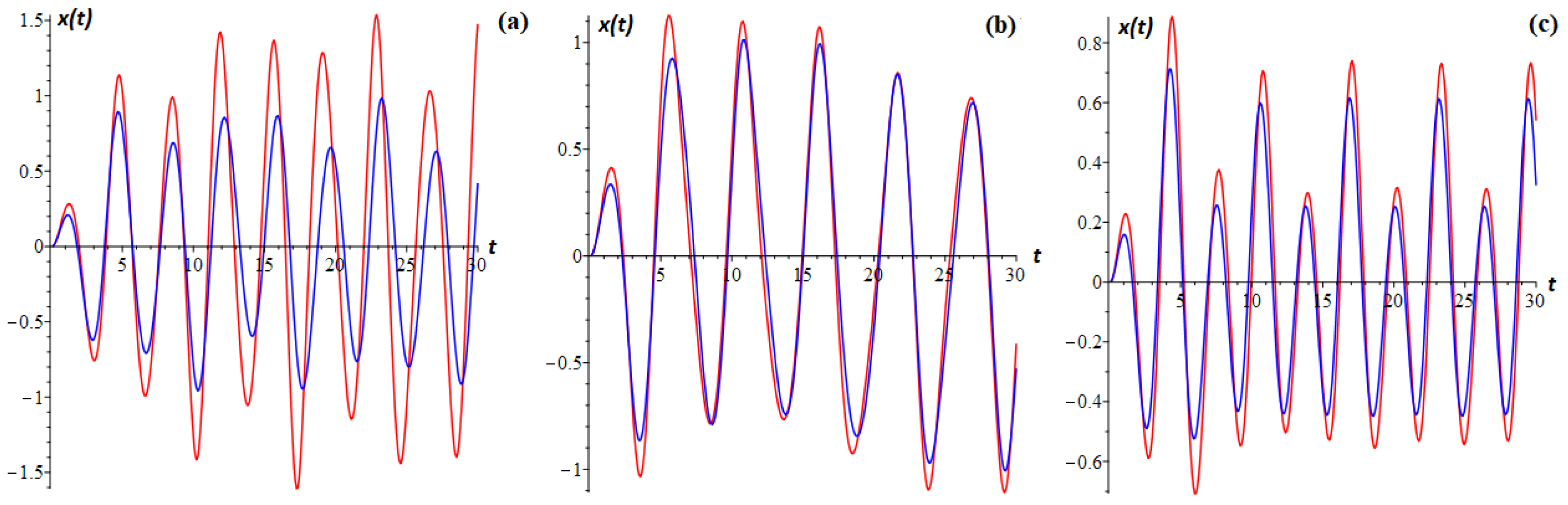
The results shown in Figure 16a–c confirm that the IFDS (8) gives more accurate results than the EFDS (7). As the frequency of the external force approaches the resonant ${\omega }_R=1.2$, the difference between the amplitude of the oscillations obtained by the IFDS and the amplitude obtained by the IFDS increases. This is clearly seen in Figure 17a–c. This behavior is related to the bistability of the Duffing oscillator.

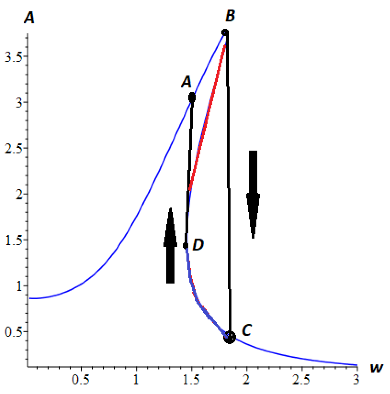
Figure 16 and Figure 18 clearly demonstrate the bistable behavior of a Duffing oscillator with a fractional derivative of variable order. When the frequency of the external force tends to the resonant ${\omega }_R$ (section AB), the amplitude of the oscillations begins to increase. Reaching the threshold value (point B), the oscillations enter an unstable mode (section BD), as a result of which the amplitude of the oscillations jumps from one stable mode to another (section BC), and then the amplitude decreases. When the frequency decreases, the amplitude increases first (CD section), then when the frequency reaches a lower resonant (point C) $\omega <{\omega }_R$, there is a jump from one mode to another (AD section). Then the amplitude decreases. The ABCD polygon is called a hysteresis loop.

The calculations in the article were carried out using the VOFDDE 1.0 software package developed in the Maple environment.

6. Conclusions

The article considered an implicit finite difference scheme (8) for the Duffing equation with a derivative of a fractional variable order of the Riemann–Liouville type. The issues of stability and convergence of the implicit finite-difference scheme were substantiated. Test cases were conducted to substantiate the theoretical results. Using the Runge rule, the results of the implicit scheme (8) were compared with the results of the explicit scheme (7). Phase trajectories and oscillograms for a Duffing oscillator with a fractional derivative of variable order of the Riemann–Liouville type were constructed, and chaotic and regular modes were studied using the spectrum of maximum Lyapunov exponents and Poincare sections. Q-factor surfaces, amplitude-frequency and phase-frequency characteristics were constructed for the study of forced oscillations. The results of the study showed that the implicit finite-difference scheme shows more accurate results than the explicit one.

References

1. Nakhushev, A.M. Fractional Calculus and Its Applications; Fizmatlit: Moscow, Russia, 2003; p. 272. (In Russian) [Google Scholar]
2. Nigmatullin, R.R. Fractional integral and its physical interpretation. Theor. Math. Phys. 1992, 90, 242–251. [Google Scholar] [CrossRef]
3. Petras, I. Fractional-Order Nonlinear Systems: Modeling, Analysis and Simulation; Springer: New York, NY, USA, 2010; p. 180. [Google Scholar]
4. Rekhviashvili, S.S.; Pskhu, A.V. A Fractional Oscillator with an Exponential-Power Memory Function. Tech. Phys. Lett. 2022, 48, 33–35. [Google Scholar] [CrossRef]
5. Syta, A.; Litak, G.; Lenci, S.; Scheffler, M. Chaotic vibrations of the Duffing system with fractional damping. Chaos Interdiscip. J. Nonlinear Sci. 2014, 24, 10–16. [Google Scholar] [CrossRef]
6. Parovik, R.I. Mathematical Models of Oscillators with Memory. Oscillators-Recent Developments; InTech: London, UK, 2019; pp. 3–21. [Google Scholar]
7. Kilbas, A.A.; Srivastava, H.M.; Trujillo, J.J. Theory and Applications of Fractional Differential Equations; Elsevier Science Limited: Amsterdam, The Netherlands, 2006; Volume 204, p. 523. [Google Scholar]
8. Zeldovich, B.Y. Optical bistability based on the orientation nonlinearity of liquid crystals. Quantum Electron. 1984, 11, 2419–2426. [Google Scholar]
9. Eskov, V.V. Chaotic dynamics of myograms. Bull. New Med. Technol. Electron. Ed. 2016, 3, 660–663. [Google Scholar]
10. Ejikeme, C.L.; Oyesanya, M.O.; Agbebaku, D.F.; Okofu, M.B. Solution to nonlinear Duffing oscillator with fractional derivatives using homotopy analysis method (HAM). Glob. J. Pure Appl. Math. 2018, 14, 1363–1388. [Google Scholar]
11. Syam, M.I. The Modified Fractional Power Series Method for Solving Fractional Undamped Duffing Equation with Cubic Nonlinearity. Nonlinear Dyn. Syst. Theory 2020, 20, 568–577. [Google Scholar]
12. Ouannas, A. Novel Control Law for the Fractional-order Chaotic Duffing Map. In Proceedings of the 2021 International Conference on Information Technology (ICIT), Amman, Jordan, 14–15 July 2021; pp. 238–241. [Google Scholar]
13. Othman, A. Different linear control laws for fractional chaotic maps using Lyapunov functional. Arch. Control Sci. 2021, 31, 765–780. [Google Scholar]
14. Xu, Y.; Li, Y.; Liu, D.; Jia, W.; Huang, H. Responses of Duffing oscillator with fractional damping and random phase. Nonlinear Dyn. 2013, 74, 745–753. [Google Scholar] [CrossRef]
15. Shen, Y.; Li, H.; Yang, S.; Peng, M.; Han, Y. Primary and subharmonic simultaneous resonance of fractional-order Duffing oscillator. Nonlinear Dyn. 2020, 102, 1485–1497. [Google Scholar] [CrossRef]
16. Xing, W. Threshold for chaos of a duffing oscillator with fractional-order derivative. Shock Vib. 2019, 2019, 1–16. [Google Scholar] [CrossRef]
17. Gao, X. Chaos in the fractional order periodically forced complex Duffing’s oscillators. Chaos Solitons Fractals 2005, 24, 97–104. [Google Scholar] [CrossRef]
18. Yang, J.H.; Sanjuán, M.A.; Wang, C.J.; Zhu, H. Vibrational Resonance in a Duffing System with a Generalized Delayed Feedback. J. Appl. Nonlinear Dyn. 2013, 2, 397–408. [Google Scholar] [CrossRef]
19. Li, Z.; Chen, D.; Zhu, J.; Liu, Y. Nonlinear dynamics of fractional order Duffing system. Chaos Solitons Fractals 2015, 81, 111–116. [Google Scholar] [CrossRef]
20. Buscarino, A.; Caponetto, R.; Fortuna, L.; Murgano, E. Chaos in a fractional order duffing system: A circuit implementation. In Proceedings of the 2019 IEEE International Conference on Systems, Man and Cybernetics, Bari, Italy, 6–9 October 2019; pp. 2573–2577. [Google Scholar]
21. El-Dib, Y.O. Stability approach of a fractional-delayed Duffing oscillator. Discontinuity Nonlinearity Complex 2020, 9, 367–376. [Google Scholar] [CrossRef]
22. Eze, S.C. Analysis of fractional Duffing oscillator. Rev. Mex. Física 2020, 66, 187–191. [Google Scholar] [CrossRef]
23. Gouari, Y.; Dahmani, Z.; Jebril, I. Application of fractional calculus on a new differential problem of duffing type. Adv. Math. Sci. J. 2020, 9, 10989–11002. [Google Scholar] [CrossRef]
24. El-Borhamy, M. Chaos transition of the generalized fractional Duffing oscillator with a generalized time delayed position feedback. Nonlinear Dyn. 2020, 101, 2471–2487. [Google Scholar] [CrossRef]
25. Ugochukwu, N.D.; Oguagbaka, M.F.; Samuel, E.S.; Aguegboh, N.S.; Ebube, O.N. On the Stability of Duffing Type Fractional Differential Equation with Cubic Nonlinearity. Open Access Libr. J. 2020, 7, 1–14. [Google Scholar] [CrossRef]
26. Barba-Franco, J.J.; Gallegos, A.; Jaimes-Reátegui, R.; Pisarchik, A.N. Dynamics of a ring of three fractional-order Duffing oscillators. Chaos Solitons Fractals 2022, 155, 111–747. [Google Scholar] [CrossRef]
27. Parovik, R.I. Dynamic hysteresis of a fractional Duffing oscillator. Bull. Inst. Math. 2019, 6, 47–51. (In Russian) [Google Scholar]
28. Li, Y.; Duan, J.-S. The periodic response of a fractional oscillator with a spring-pot and an inerter-pot. J. Mech. 2020, 37, 108–117. [Google Scholar] [CrossRef]
29. Ma, R.; Zhang, B.; Han, J. Bifurcation analysis of fractional duffing system based on improved short memory principle method. J. Vibroeng. 2022, 24, 1162–1173. [Google Scholar] [CrossRef]
30. Sun, H.; Chang, A.; Zhang, Y.; Chen, W. Variable-order fractional differential equations: Mathematical foundations, physical models, numerical methods and applications. Fract. Calc. Appl. Anal. 2019, 22, 27–59. [Google Scholar] [CrossRef] [Green Version]
31. Meerschaert, M.M.; Tadjeran, C. Finite difference approximations for fractional advection–dispersion flow equations. J. Comput. Appl. Math. 2004, 172, 65–77. [Google Scholar] [CrossRef] [Green Version]
32. Zhuang, P.; Liu, F.; Anh, V.; Turner, I. Numerical methods for the variable-order fractional advection-diffusion equation with a nonlinear source term. SIAM J. Numer. Anal. 2009, 47, 1760–1781. [Google Scholar] [CrossRef]
33. Parovik, R.I. Mathematical modeling of linear fractional oscillators. Mathematics 2020, 8, 1879. [Google Scholar] [CrossRef]
34. Yang, C.; Liu, F. A computationally effective predictor-corrector method for simulating fractional-order dynamical control system. ANZIAM J. 2006, 47, 168–184. [Google Scholar] [CrossRef] [Green Version]
35. Kim, V.A. Duffing oscillator with an external harmonic impact and derived variables fractional Remann-Liouville, is characterized by viscous friction. Bull. KRASEC Phys. Math. Sci. 2016, 13, 46–49. [Google Scholar]
36. Kim, V.A.; Parovik, R.I. Some aspects of the numerical analysis of a fractional duffing oscillator with a fractional variable order derivative of the Riemann-Liouville type. AIP Conf. Proc. 2022, 2467, 060014. [Google Scholar]
37. Kim, V.A.; Parovik, R.I. Calculation of maximum Lyapunov exponents for an oscillatory Duffing system with power-law memory. Bull. KRASEC Phys. Math. Sci. 2018, 23, 98–105. [Google Scholar]
38. Hioual, A.; Ouannas, A.; Oussaeif, T.-E.; Grassi, G.; Batiha, I.M.; Momani, S. On Variable-Order Fractional Discrete Neural Networks: Solvability and Stability. Fract. Fractals 2022, 6, 119. [Google Scholar] [CrossRef]
39. Kim, V.A.; Parovik, R.I. Application of the Explicit Euler Method for Numerical Analysis of a Nonlinear Fractional Oscillation Equation. Fract. Fractals 2022, 6, 274. [Google Scholar] [CrossRef]
40. Kim, V.A.; Parovik, R.I. Investigation of forced oscillations of a Duffing oscillator with a derivative of a variable fractional Riemann-Liouville order. Proc. Kabard.-Balkar. Sci. Cent. Russ. Acad. Sci. 2020, 93, 46–56. [Google Scholar]
41. Kim, V.A.; Parovik, R.I. Mathematical model of fractional Duffing oscillator with variable memory. Mathematics 2020, 8, 2063. [Google Scholar] [CrossRef]
42. Parovik, R.I. Existence and uniqueness of the Cauchy problem for a fractal nonlinear oscillator equation. Uz. Math. J. 2017, 4, 110–118. [Google Scholar]
43. Wolf, A.; Swift, J.B.; Swinney, H.L.; Vastano, J.A. Determining Lyapunov exponents from a time series. Phys. Nonlinear Phenom. 1985, 16, 285–317. [Google Scholar] [CrossRef] [Green Version]
44. Wawrzynski, W. The origin point of the unstable solution area of a forced softening Duffing oscillator. Sci. Rep. 2022, 12, 4518. [Google Scholar] [CrossRef]
Figure 1. Solutions of the Cauchy problem (1) obtained from schemes (7) and (8), as well as the exact solution (12).
Mathematics 11 00558 g001
Figure 2. (a) Error ε , (b) computational accuracy α .
Mathematics 11 00558 g002
Figure 3. Solutions of the Cauchy problem (1) obtained from schemes (7) and (8), as well as the exact solution (12). For the EFDS (7), the conditions of Theorems 1 and 2 are violated.
Mathematics 11 00558 g003
Figure 4. (a) Error ε , (b) computational accuracy α .
Mathematics 11 00558 g004
Figure 5. Phase trajectory (a) and waveform (b) for the Cauchy problem (1) obtained by explicit (7) and implicit (8) schemes.
Mathematics 11 00558 g005
Figure 6. (a) Error ε , (b) computational accuracy α .
Mathematics 11 00558 g006
Figure 7. (a) Error ε , (b) computational accuracy α . The conditions of Theorems 1 and 2 are violated.
Mathematics 11 00558 g007
Figure 8. (a) Phase trajectories at λ = 0.18 , (b) the spectrum of Lyapunov exponents from λ and (c) phase trajectories at λ = 0.6 . The dots represent the Poincare sections.
Mathematics 11 00558 g008
Figure 9. (a) Phase trajectories at q = 0.15 , (b) the spectrum of Lyapunov exponents from q and (c) phase trajectories at q = 0.6 . The dots represent the Poincare sections.
Mathematics 11 00558 g009
Figure 10. Phase trajectory (a) and waveform (b) for the Cauchy problem (1) obtained by explicit (7) and implicit (8) schemes.
Mathematics 11 00558 g010
Figure 11. (a) Phase trajectories at λ = 0.1 , (b) the spectrum of Lyapunov exponents from λ and (c) phase trajectories at λ = 0.4 .
Mathematics 11 00558 g011
Figure 12. Phase trajectory (a) and waveform (b) for the Cauchy problem (1) obtained by explicit (7) and implicit (8) schemes.
Mathematics 11 00558 g012
Figure 13. (a) Phase trajectories at λ = 0.1 , (b) the spectrum of Lyapunov exponents from λ and (c) phase trajectories at λ = 0.4 .
Mathematics 11 00558 g013
Figure 14. (a) AFC and (b) PFC for operator (2) with order q ( t ) = 0.8 cos ( 0.5 t ) .
Mathematics 11 00558 g014
Figure 15. Q factor: (a) q ( t ) = 0.8 cos ( 0.5 t ) , (b) for q [ 0 , 1 ] .
Mathematics 11 00558 g015
Figure 16. Numerical and analytical AFC of the fractional Duffing oscillator for various types of function q ( t ) .
Mathematics 11 00558 g016
Figure 17. Waveforms for q ( t ) = 0.8 cos ( 0.5 t ) at (a) ω = 1.2 , (b) ω = 1.5 and (c) ω = 1.9 .
Mathematics 11 00558 g017
Figure 18. Hysteresis loop. The resonance curve is marked in blue. The part of the resonance curve where the frequency jump occurs is highlighted in red.
Mathematics 11 00558 g018
Disclaimer/Publisher’s Note: The statements, opinions and data contained in all publications are solely those of the individual author(s) and contributor(s) and not of MDPI and/or the editor(s). MDPI and/or the editor(s) disclaim responsibility for any injury to people or property resulting from any ideas, methods, instructions or products referred to in the content.