The Extended David-Yechiali Rule for Kidney Allocation

Abstract

The First Come First Served (FCFS) queuing policy is routinely assumed to be the benchmark policy for “fairness” in waiting-time performance. In this article, we propose a slight modification of the FCFS policy based on a natural extension of the well-established David and Yechiali (DY) rule and analyze it in the context of managing a waiting list for kidney transplants. In the proposed policy, the queuing agents are sequentially offered a stochastically arriving organ on a “first come, first served” basis while applying the individually optimal DY stopping rule. Through a realistic simulation, we show that the proposed policy, which we term Extended David and Yechiali (EDY), favorably compares to the FCFS policy in terms of medical efficiency while maintaining a comparable level of equity (i.e., fairness). Possible implications and practical aspects of the EDY are discussed.

1. Introduction

Kidney transplantation is the most effective treatment for End Stage Renal Disease (ESRD) patients. Without transplantation, patients must undergo dialysis treatments to survive [1]. However, the kidney supply for transplantation is insufficient to meet the increasing demand. According to a recent study [2], at the start of 2019, 100,998 adult patients had been waiting for a kidney transplant. During that year, 42,934 patients were added to the waiting list, while the total number of kidney transplants performed during that period was only 24,273. Even in the unlikely case of sufficient (or excess) kidneys for all patients, one is still faced with a complex allocation problem. Namely, a specific kidney is not suitable for all candidate patients, and even if it is, it is rarely a “perfect match”. Thus, from the potential recipient’s perspective, the question is whether s/he “wants” a given kidney or prefers to wait for the next one (if and when one becomes available).

Managing an organ transplant waiting list is a highly complex process guided by several factors that do not necessarily align. These include (1) medical urgency (e.g., how long can a person survive without a transplant?), (2) donor-recipient compatibility (e.g., donor-recipient ethnicity, age, blood type, etc.), (3) logistical factors (e.g., geographical distance between the available organ and the recipient) and (4) fairness considerations (e.g., is there another candidate that has waited longer in the queue?), to name a few [3]. While many allocation policies were proposed in the literature, one of the key ongoing challenges in determining an appropriate organ allocation policy is the inherent possible trade-off between clinical efficiency and equity. Simply put, clinical efficiency and fairness might be partially conflicting since a clinically efficient allocation may be arbitrarily far from any definition of a fair allocation. Moreover, while clinical efficiency is often measured by standard metrics such as the QALY (Quality Adjusted Life Years), there is currently no consensus measure for fairness.

This paper builds on the theoretically grounded David and Yechiali (DY) optimal stopping rule [4]. The rule is devised for the simple case in which only a single candidate patient waits for a kidney transplant. The candidate needs to decide if s/he wants to accept a stochastically arriving organ or if s/he prefers to refuse a given organ and wait for a (hopefully) better one to arrive in the future. In the real world, where organs are a scarce resource compared to the number of waiting patients, the DY rule does not readily apply. Therefore, in this study, we propose and investigate a serial version of the DY rule that we term the Extended David-Yechiali (EDY) policy. The EDY works iteratively. Once a kidney arrives, it is offered to the first candidate in the queue (ordered by registration, as in the FCFS policy). Then, the candidate applies the DY rule as if s/he were the only patient in the queue. If the organ is rejected, the kidney is offered to the next candidate in the queue, and so on. Clearly, applying the DY rule in this way is not necessarily optimal for a candidate who is not the first in line, as it does not explicitly account for the (likely) possibility that other candidates will accept future arriving organs before they are offered to that candidate. Given the decentralized manner in which most organ allocation policies are applied (i.e., candidates are unaware of other registered candidates’ characteristics and preferences), it seems unreasonable to assume that candidates can effectively make “fully rational” strategic decisions that account for the complete profile of other candidates in the system [5]. Alternatively, in the proposed EDY, the individually applied DY rule is sensitive to the arrival rate of organs for each candidate in the queue separately. As such, in the EDY policy, each candidate implicitly considers the preferences of other candidates in the system practically.

Since there is no consensus measure for fairness, it is common to compare any given allocation policy to the benchmark “First Come, First Served” (FCFS) policy, routinely assumed to be the gold standard for fairness (e.g., [6]). Thus, simulation is a practical way to represent the dynamic nature of organ allocation and address the multi-faceted challenge of determining whether one organ allocation policy is preferable to another [7]. Hence, in this work, we investigate the proposed EDY policy using a realistic simulation and compare it to the classic FCFS.

Our results show that the EDY policy seems to strike a reasonable compromise between clinical efficiency and fairness. The average and standard deviation of waiting times is almost identical to the classic FCFS policy while receiving a more biologically suitable kidney, thus improving candidates’ longevity.

The paper is organized as follows:

• Section 2 commences by discussing the issue of fairness in queues and the FCFS policy, then introduces several efficiency measures on our work and the efficiency determinants in transplantation. It also discusses the DY rule and its characteristics.
• Section 3 defines the EDY policy, which is the focus of this work.
• Section 4 demonstrates an overview of the simulation model and exhibits the model assumptions. We developed a loop-time-based simulation engine to implement the model using Python based on statistical data from the OPTN [2]. In addition, the section displays the methodology of comparison.
• Section 5 presents the simulation results.
• Section 6 depicts the conclusion.

2. Background

2.1. Fairness and Efficiency

The concept of fairness in queueing systems is a topic of ongoing debate and research. In the context of kidney allocation, many studies have compared different allocation policies to the classic First-Come-First-Served (FCFS) policy, which is often used as a benchmark for fairness. In addition to fairness, clinical efficiency is essential in organ allocation. Factors that impact the success of kidney transplantation can be divided into two main categories: mandatory factors and chance factors. Mandatory factors include the compatibility of the donor and recipient’s ABO blood types and the availability and willingness of the recipient to undergo transplantation. Chance factors include the compatibility of the donor and recipient’s HLA tissue type and the PRA score of the recipient. These and other factors must be considered in order to develop effective and fair organ allocation policies.

Unfortunately, determining how to combine these and other similar measures into a single score is an ongoing challenge. One possible solution, which we advocate for in this article, is delegating the decision to accept or reject a given organ to the candidates, thus allowing for flexibility and distributed decision process. To that end, we propose a natural extension of the DY rule, as discussed next.

2.2. The David-Yechiali Rule

David and Yechiali [4] studied a time-dependent stopping problem and its application to the decision-making process associated with organ transplanting. The DY rule changes the traditional standpoint, and instead of examining who is the right candidate for a given organ, they scan for the appropriate organ for a specific candidate. The researchers assume only one candidate is in the system; therefore, the rule is called “The Single Candidate problem”.

The DY rule works as follows. When an organ arrives, a decision about whether to accept it or not is made based on the “value” of that organ and the prospective expected “value” of waiting for a (hopefully) better one in the future. If the organ is accepted, the process terminates, and the candidate goes through the transplantation process. Otherwise, the offer is lost, and the process continues until the next kidney arrives or until the candidate dies. The rule is illustrated in Figure 1.

In the original paper, the authors assumed that candidates base their decision on three known parameters: (1) the inter-arrival time, (2) the HLA distribution, and (3) the blood type distribution. According to these parameters, the candidates calculate the time they are willing to wait for each matching level.

3. The Extended David-Yechiali Policy

The DY rule was designed for an organ allocation system with only a single candidate. However, more than a single candidate is registered in the system in realistic settings. Thus, we propose a natural serialization of the DY rule, which applies to any number of candidates. We refer to the resulting policy as the Extended David-Yechiali (EDY) policy. The policy is depicted in Figure 2.

The policy states that when a kidney arrives, it is offered to the first candidate (based on their registration time in the system). Then, the candidate is screened to ensure the mandatory efficiency factors are met (see Section 2.1). If the candidate does not pass the screening, the offer is considered “rejected” and the kidney is offered to the next candidate in line, and the process is repeated. Otherwise, the candidate calculates the time s/he is willing to wait for each matching level as per the DY rule. If the candidate accepts the offer, the transplant takes place, and the candidate leaves the queue. Otherwise, the kidney is offered to the next candidate, and the process is repeated. In the unrealistic case where all candidates are incompatible and reject the organ, the process terminates and waits for the next available organ.

Naturally, for the first candidate in the queue, the EDY policy entails a simple “single candidate” setting where the applied DY rule is known to be optimal. However, if the candidate is not first on the list, the DY rule does not explicitly consider that future arriving organs could be taken by one of the candidates that stand before them on the list. Nevertheless, it is essential to note that the DY rule is applied separately for each individual in the queue. Specifically, each candidate’s organs’ arrival rate is directly influenced by the candidates’ decisions who stand before them in the queue. Therefore, the decision is calculated differently for each candidate and implicitly accounts for their preferences.

4. Evaluation

We use simulation to evaluate the proposed EDY policy. The simulation consists of several components discussed next, followed by the main results and their interpretation.

4.1. EDY Implementation

Our EDY implementation uses the classic FCFS strategy to rank the candidates in the queue.

As for a screening strategy, we follow the standard practice and perform a blood type matching test, a negative crossmatch test and check whether the candidate is available for transplant at the current time.

As in the original DY rule, we assume that the lifetime distribution of kidneys is Gamma with shape parameter $\alpha =2$ and scale parameter $\theta =1/2.5$ (normalization for 2.5 years’ time-period). We calculate the minimal time to accept the current offer (see Appendix A); the effective average fit kidney for a specific candidate depends on two personal parameters and is calculated as follows:

$${\mu }_{eff}=P_{blood}\cdot P_{location}\cdot \mu$$

where:

$\mu$ is the donor’s yearly arrival rate.

$P_{blood}$ is the probability of finding a compatible blood type kidney. For example, if the candidate’s blood type is A, s/he can accept a kidney with A or O blood type.

$P_{location}$ is the arrival rate for each candidate according to the place on the waiting list. The $P_{location}$ of the first candidate is 1 because all the offers pass through him/her.

For example, assuming the average kidney arrival rate is 100 per year and a candidate with blood type A is placed on the 20th slot in the waiting list; the candidate’s actual kidney arrival rate is 17.5 per year: if 30% of the population have an O blood type and 40% have an A blood type, the $P_{blood}$ of the candidate is 0.3 + 0.4 = 0.7, and if the 20th place in line receives only 25% of the offers, the $P_{location}$ is $0.25$; then, the actual rate that the candidate considers is 0.7 · 0.25 · 100 = 17.5.

4.2. FCFS Implementation

We compare the EDY policy to the classic FCFS policy. In our FCFS implementation, when a kidney enters the system, it is allocated to the first candidate in the queue that is a suitable match (i.e., passes the screening test). In our context, the FCFS is considered the gold standard for fairness.

4.3. Core Models

We constructed a modular simulation model that mimics the operation of a real allocation system.

The implementation consists of four supporting components and eight key components for the kidney transplant model in

Table 1. The simulation’s components. Bolded headers represent the context of the component in the simulation.

Candidates	Initialization Candidate Generation Candidate Aging Waiting-list Death Post-Transplant	Kidneys	Donor Generation Kidney Expiration
		Process	Organ Allocation Statistics Metrics
Support	Simulation Engine	Settings	Bio-Data	Logging

:

4.3.1. Supporting Components

The simulation engine component is based on a loop that advances time (steps) using the simulation time unit (default: days). The simulation ends when the time advances to the total time. Events’ timing is normalized to the “whole” step, e.g., if a candidate is to arrive at time $t=2.2$, it will occur at the $t=3$ step.

The settings components read the settings from a file and provide them for all the other components. The available settings are detailed in Appendix B.

The bio-data component includes all biological data (based on OPTN) and logic.

The logging component writes logs to a file that can be read afterward to evaluate the simulation’s run.

4.3.2. Kidney-Transplant Components

All key components are registered to the simulation engine and have a process function that will be invoked at each step of the simulation.

The candidates’ initialization component is based on the OPTN data report. We initialize a set of candidates before the simulation starts with distributed waiting times.

The candidate generation component is based on the OPTN data report. We set the candidates’ arrival times using an exponential distribution and generate synthetic data for each candidate, e.g., age, blood type, gender, etc. (Appendix D).

The candidate aging component: each candidate arrives at the model at a specific time and age, and as the simulation advances, the age changes appropriately. If a candidate becomes too old for transplantation, s/he is removed from the system.

The waiting-list death component: in our model, we simulate a patient’s death on the waiting list. According to [2], 6.8% died while waiting between 2016 and 2019. To simulate that, we set inter-arrival death time:

$$\mathrm{Interarival}-\mathrm{time}=\frac{365}{\left(\mathrm{Candidates} \mathrm{queue} \mathrm{length}\right)\cdot 0.068}$$

When the time comes and death occurs, we remove a random patient from the waiting list. In our model, we assume that all patients on the waiting list have an equal chance of dying, regardless of their attributes (age, health condition, etc.). The health condition, a crucial factor, is not considered in the simulation, as it is unknown to us.

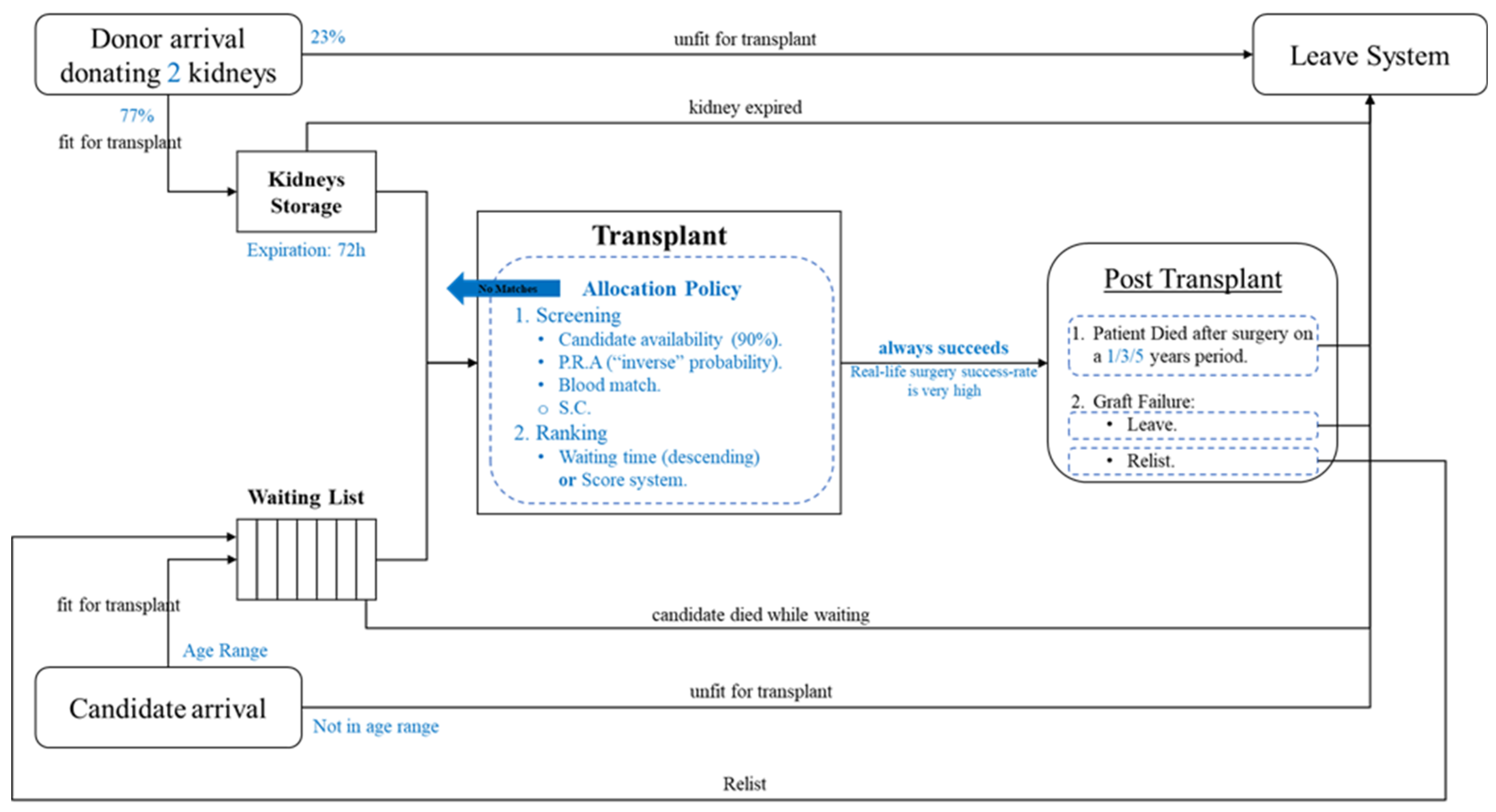
The post-transplant component: over time, two events can occur after a kidney is transplanted into a candidate. (1) organic death (death of a patient with a functioning graft) leading to leaving the system or (2) organ failure, which can result in a re-list (putting the patient back on the waiting list) or in a decision to leave. The transplanted candidates have a checkup period of 1 year, and we simulate the events for expanded times (next year).

The donor generation component: this is based on the OPTN data report. We set the donors’ arrival times using an exponential distribution and generate synthetic data, e.g., blood type, antigens, gender, etc. For each donor, two kidneys are extracted, but only a portion is fit for transplant; in our simulation, only 77% of the kidneys are suitable for transplant.

The kidney expiration component: in our model, we simulate the shelf-life of an extracted kidney. Each kidney is available for 72 h after extraction (donor arrival time). When the kidney’s shelf-life passes, it is removed from the organ storage (leaving the system) and cannot be allocated anymore.

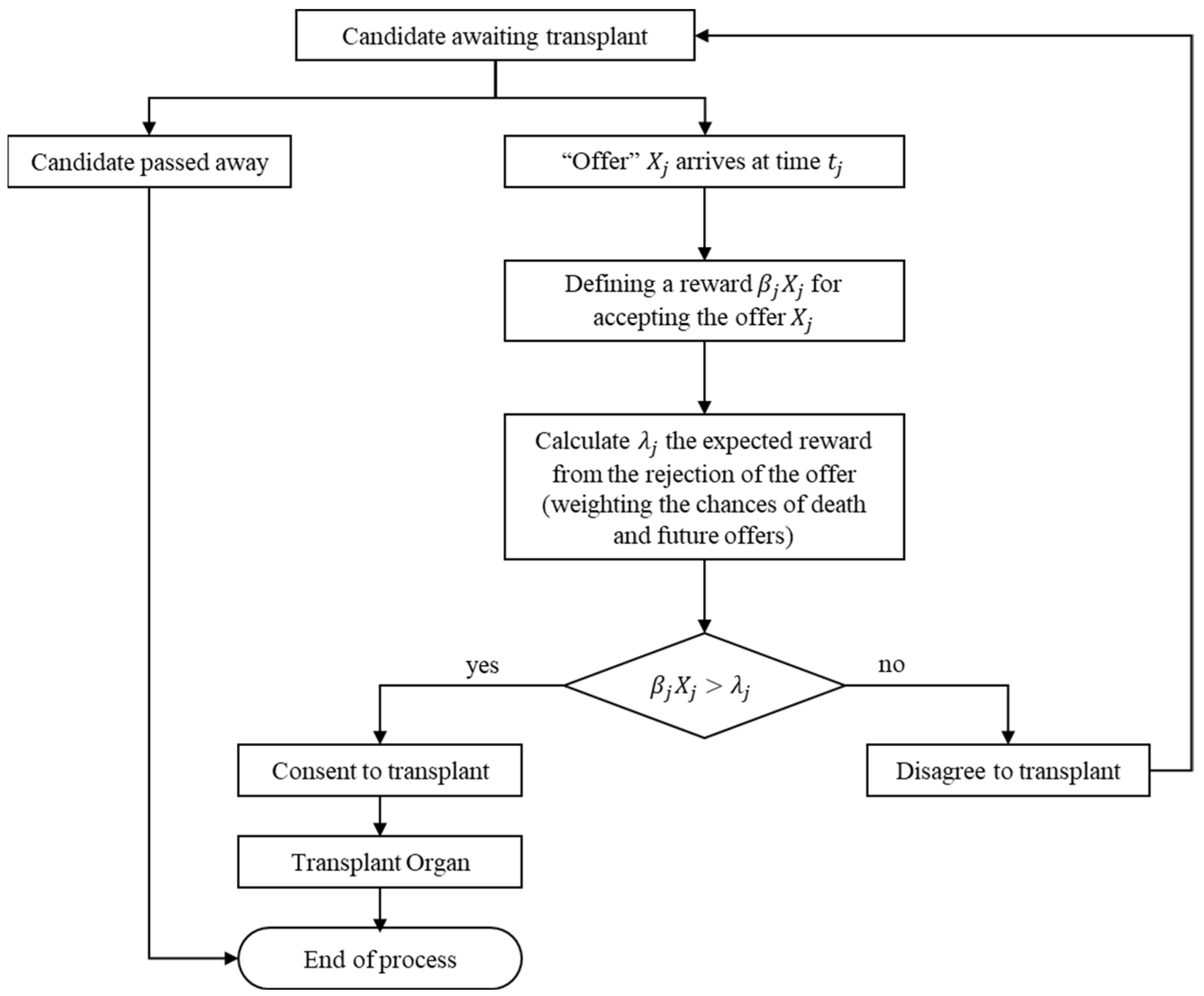
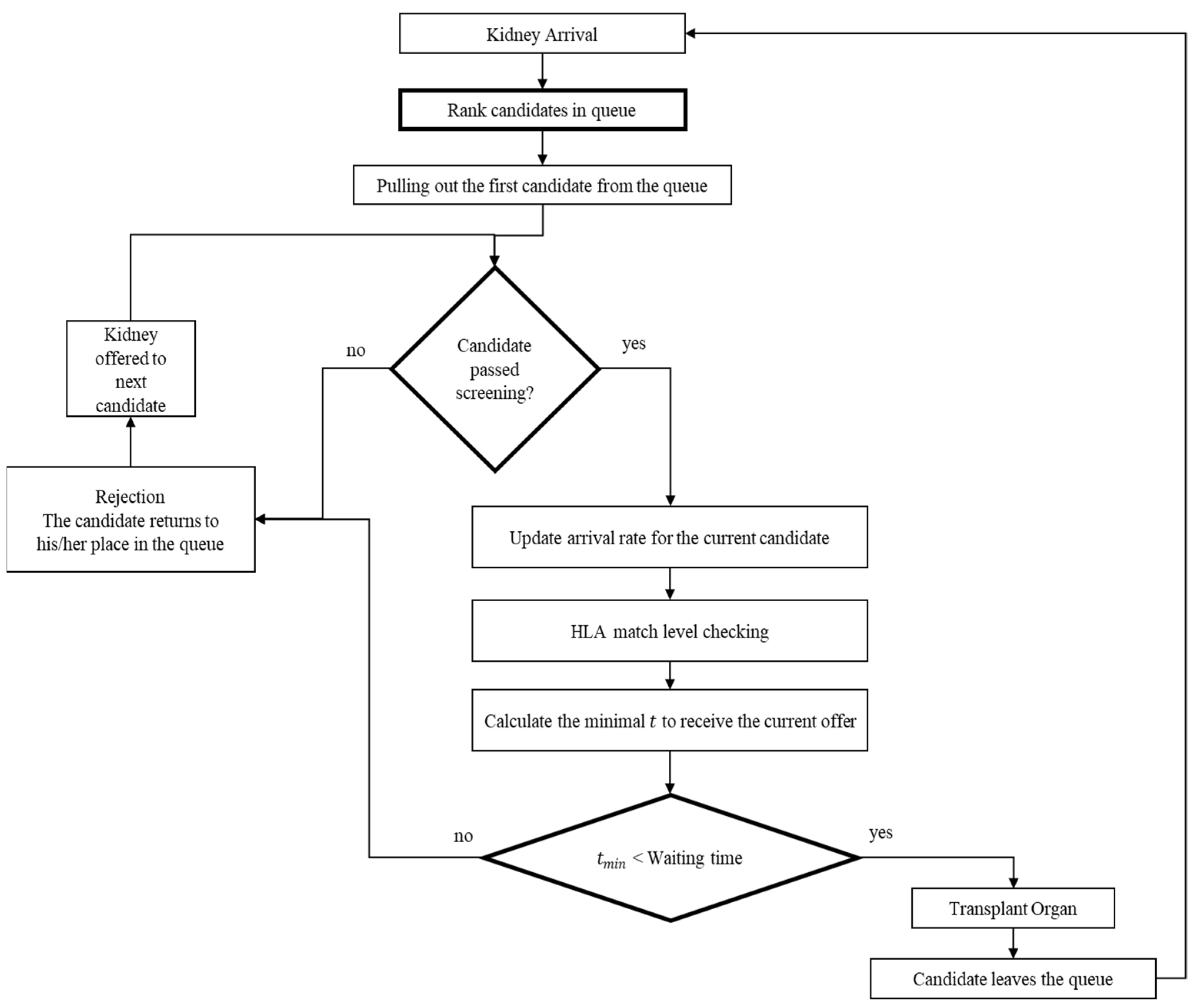
The organ allocation component: the waiting list is sorted by the patient’s arrival time in this model. According to EDY, the organ is offered to the first candidate on the waiting list. Then three actions are performed: in the first stage, the kidney blood type compatibility with the candidate is checked. The second step, called “crossmatch”, must be passed for the candidate to accept the kidney. The third step is the “candidate decision”. The candidates contemplate if they should accept the offer (kidney) and leave the system or wait for the next arrival. This decision is made using mathematical calculations that combine the “single-candidate algorithm” and EDY. If the kidney successfully goes through those three steps, the candidate receives the kidney and leaves the waiting list. If it does not, the next candidate on the list goes through the above steps. Finally, if none of the candidates decides to take the kidney before it passes its shelf-life, it is disposed of and logged in a file.

The statistics component: at the end of each step of the simulation (default: end of the day), we generate statistics for waiting times, waiting-list size, number of deaths, number of arrivals, etc. Additional data during the simulation is recorded using “recorders”, based on an observer design pattern for each component.

The metrics component: at the end of each simulation step (default: end of the day), we record the data needed to calculate metrics (for clinical efficiency and equity) at each segment.

For statistical analysis of the results, we divided the simulation into 20-time segments, so the calculation of each metric refers only to the specific time segment and not to the ones before it.

4.3.3. Further Assumptions

The lifetime distribution of kidneys is Gamma with shape parameters $\alpha =2$ and the scale parameter $\theta =1/2.5$. To simplify calculations, we assume $\theta =1$, bearing in mind that the time unit is 2.5 years. μ is the rate of kidney offers for 2.5 years.

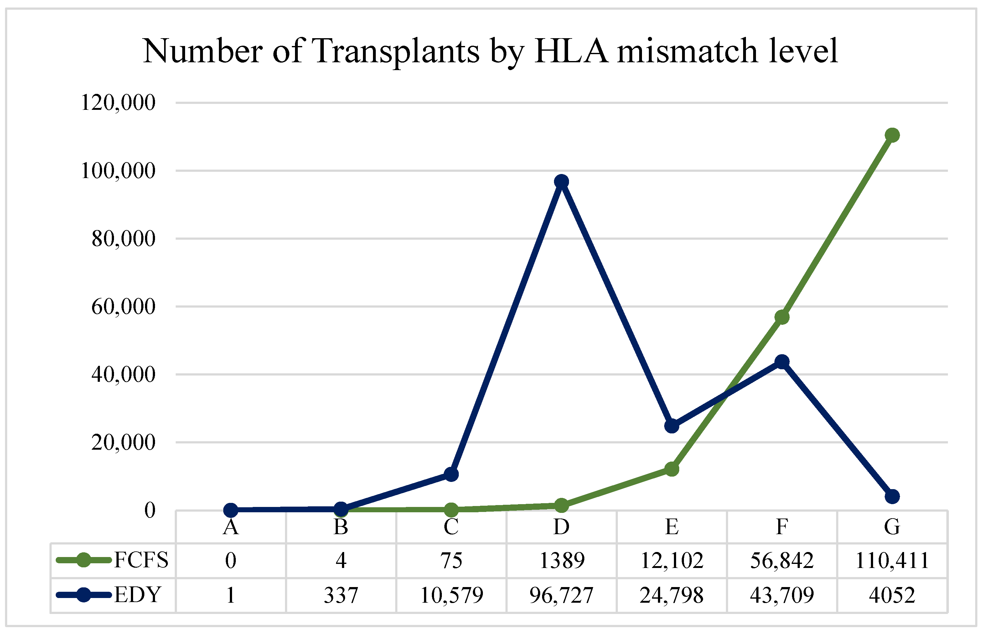
Each kidney arrival results in an A, B, C, D, E, F, or G Match, as in

Table 2. Graft survivability probability within one year per HLA mismatch level according to the OPTN.

HLA Mismatch Level	X (%)
0 HLA MM	96
1 HLA MM	96.7
2 HLA MM	96.2
3 HLA MM	95.5
4 HLA MM	94.4
5 HLA MM	94.1
6 HLA MM	93.4

.

Table 3. Blood type frequency in the US population according to the OPTN annual report.

Blood Type	Frequency in the Population (%)
A	27.3
B	16.7
AB	2.5
O	53.5

depicts the blood type distribution according to the OPTN website.

It is important to note that candidates unavailable when the kidney arrives are not considered. Furthermore, candidates, organs’ attributes, and arrival times are taken from OPTN’s past data. The PRA of the candidates does not change during the simulation. Matching the blood type is performed according to

Table 4. Blood type compatibility matrix.

Blood Type	Can Receive a Donation from Blood Types:	Can Donate to the Following Blood Types:
A	A, O	A, AB
B	B, O	B, AB
AB	A, B, AB, O	AB
O	O	A, B, AB, O

.

When death is supposed to occur, a random candidate is chosen and removed from the waiting list. Additionally, rejection will not cause a candidate who underwent a kidney transplant to return to the waiting list.

4.4. Implementation Summary

In order to run our model, we developed the simulation of the system operation in Python and based our synthetic data generation on the statistics of the OPTN data reports. Figure 3 summarizes the model implementation:

4.5. Evaluation Metrics

During each simulation run, 430,000 candidates joined the waiting list (starting with 100,000 patients), and only 180,000 transplantations were performed over 3660 days (the number of days closest to 10 years divided into 20-time segments giving a whole number, 183 days per segment). According to the OPTN data reports [2], over 40,000 applicants join the kidney transplant waiting list every year. In addition, to test the effect on the quality of life over five years between transplant and the time of death, we will perform a twice as long (10 years) simulation. The results exhibit equity and clinical efficiency, waiting time STD, and the number of transplantations for any match level (A to G), as discussed next.

4.5.1. Clinical Efficiency

Clinical efficiency measures the suitability between a kidney and a particular candidate. If an allocation process is chiefly based on stringent suitability criteria, the chances for successful transplantation will increase (yet the number of transplants may decrease). We consider two standard metrics: (1) The Graft survivability percentage; and (2) Discounted QALYs. Starting with Graft survivability, as was discussed in Section 2.1, a better HLA match does not mean only a better chance of survival. It also means improved patient general health. When patients receive a kidney with a better match, they do not need to use as many medications targeted toward the immune system; thus, their chance of catching another disease is reduced. As for the discounted QALY, quality-adjusted life years measure the value of health outcomes [6]. The higher the metric, the better the medical effectiveness of the allocation policy. Zenios et al. [6] claim that when calculating the value of QALYs, it is customary to use the discounting of the value on the assumption that the value of a current year is higher than the value of a future year. In this study, discounting is carried out using the discount factor, calculated as follows: $\frac{1}{{(1+r)}^{T_{now}}}$, where $r$ is the daily interest, and $T_{now}$ is the current time in the system, i.e., the time that has passed since the start of the simulation. According to the assumption, the QOL (quality of life) score for waiting candidates is 0.65, the QOL score for transplanted candidates is 0.7, and the daily interest rate is 0.014%. The calculation is performed the same way as the undiscounted QALYs index, but each index update is multiplied by the discount factor.

4.5.2. Fairness and Equity

The average waiting time in a queuing system is, arguably, the most logical metric for measuring fairness. However, in our setting, this is not necessarily correct. This is due, in part, to the fact that the service time (performing the allocation and kidney transplant surgery) is negligible, and the average waiting time is only measured according to the candidates who have already had enough time to receive the service (i.e., transplant). Specifically, this metric does not consider candidates who died while waiting or are still waiting for a kidney. Although one of the system’s outputs is average waiting time, this metric should be treated with caution.

The regular calculation of average waiting time is, $\frac{{{\displaystyle \sum }}_{i=1}^n(x_{transplant}^i-x_{arrival}^i)}{n}$, where $x_{arrival}^i$ is the arrival time of candidate $i$, $x_{transplant}^i$ is the time of performing the transplant of candidate $i$, and $n$ is the number of transplanted candidates. As explained, the regular average waiting time does not consider candidates still waiting in line or candidates who died while waiting. Therefore, we would like to partially correct the distortion in the revised average waiting time. The revised calculation is as follows: $\frac{{{\displaystyle \sum }}_{i=1}^m{x}_{waiting time}^i}{m}$ where $x_{waitingtime}^i=\{\begin{array}{ll}{x}_{transplant}^i-x_{arrival}^i\hfill & \mathrm{transplanted}\hfill \\ x_{dead}^i-x_{arrival}^i\hfill & \mathrm{dead}\hfill \\ T_{END}-x_{arrival}^i\hfill & \mathrm{still\; waiting}\hfill \end{array}$, $x_{dead}^i$ the death time of candidate $i$, $m$ is the number of total candidates and $T_{END}$ is the ending time of the simulation. If the candidate manages to receive a transplant, the waiting time is equal to the time from the moment of arrival until the transplant is performed. If the candidate dies while waiting, his/her waiting time is equal to the time from the moment of arrival until death. If the simulation is over and the candidate has not yet received a kidney, his/her waiting time is equal to the time from the moment of arrival until the end of the simulation.

Based on the above definition of waiting time, we consider two standard metrics: (1) The standard deviation of a candidate’s waiting time in the queue; and (2) The WTI (according to Equation (11) in [6]). The WTI index is quite similar to the standard deviation index; however, it is calculated between groups, while the standard deviation is calculated among individuals. For instance, say we divide the population into 13 groups. Concerning the WTI index, closer average waiting times within a group translate to a lower WTI index, meaning a better WTI index.

It is important to note that other fairness measures exist other than waiting time. For instance, patient age is a known parameter often connected with fairness. Namely, when a donation is given, a younger candidate should be preferred over an older one. Nevertheless, we do not use the patient’s age parameter in our allocation policy and leave the investigation of other measures for future work.

Another way to examine EDY waiting time fairness is by the waiting time std. error parameter. While checking waiting time results, there are two parameters: average waiting time and waiting time STD. In a regular queuing system, average waiting time could be relevant. However, in this kind of queuing system, it is not because the average waiting time depends on a parameter that cannot be changed: the donor arrival times. In each candidate arrival rate and a given donor arrival rate, the average waiting time will be the same, no matter what our allocation policy is, as long as we assume that when the simulation ends, all the candidates receive kidneys, and none die. The only result that changed from one policy to another is the waiting time STD error. Let’s examine a hypothetical case in which all the candidates received a kidney after precisely three years. In this case, the waiting time STD error is 0, the best possible result.

Authors should discuss the results and how they can be interpreted from the perspective of previous studies and of the working hypotheses. The findings and their implications should be discussed in the broadest context possible. Future research directions may also be highlighted.

5. Results

5.1. Clinical Efficiency

We compare the allocation policies according to the matching level metric. The comparison is provided in

Table 5. Transplants Graft Survival per HLA mismatch level.

	FCFS			EDY
HLA Mismatch Level	Transplants	At Least 5 Years	Percentage	Transplants	At Least 5 Years	Percentage
A	0	0	-	1	1	100.00%
B	4	3	75.00%	337	112	33.23%
C	75	25	33.33%	10,579	3461	32.72%
D	1389	390	28.08%	96,727	29,095	30.08%
E	12,102	3277	27.08%	24,798	6234	25.14%
F	56,842	14,582	25.65%	43,709	10,961	25.08%
G	110,411	27,787	25.17%	4052	1309	32.31%
Total	180,823	46,064	25.47%	18,0203	51,173	28.40%

Note: The difference in survivability percentage on the same HLA mismatch level is probably due to the differences in the number of samples since a higher number of samples can lead to more accurate data and analysis. This is especially evident at levels D and G, where most samples are found in EDY and FCFS, respectively.

. In this table, each row represents an HLA mismatch level. The columns for each allocation method are the number of transplants, the number of transplant patients who survived at least five years, and the percentage of survivors. The total, without the division to HLA mismatch levels, for each allocation policy is shown in the last row and the numbers in bold indicate statistical significance at p < 0.05.

5.1.1. Graft Survivability Percentage

Graft survivability percentage refers to the percentage of candidates that enjoyed longevity and survival of the graft for at least five years after transplantation.

In the comparison between FCFS and EDY in Table 5, one can see that the percentage of graft survival is statistically significantly higher in the latter policy (last row). This is due to the distribution of transplants between the matching levels, as shown above. Although the difference is not significant in nominal terms (~3%), it is substantial compared to the differences in the chance of graft survival (approx. 7.1% difference between 0 and 6 HLA mismatches after five years; Appendix C rows in bold). In the FCFS policy, clinical efficiency is not directly considered, resulting in fewer transplants with good match levels and many low-quality transplants. In the FCFS policy, 99.19% of allocations are made at match levels E, F, and mostly G (over 60%). On the other hand, as seen in Figure 4, using the EDY policy, ~70% of the allocations are made around the D level (C, D, and E), and most of the rest (over 25%) are made in F and G levels.

5.1.2. Discounted QALY’s Index

In the simulation, each segment calculates the Discounted QALYs’s score. This score is divided by the number of days in each segment to receive the Discounted QALYs’ daily average.

According to the simulation’s results in

Table 6. Discounted QALY’s index per segment in the simulation.

Mean Discounted QALY
Segment	FCFS	EDY
1	68,946.33	68,855.13
2	78,408.71	78,335.45
3	86,128.19	86,037.84
4	93,481.47	93,567.76
5	99,485.48	99,690.60
6	105,197.91	105,386.73
7	109,833.45	110,054.88
8	114,122.82	114,374.40
9	117,557.81	117,850.93
10	120,528.18	120,932.28
11	123,070.99	123,513.04
12	125,201.04	125,787.35
13	126,828.27	127,541.87
14	128,307.62	129,064.10
15	129,547.66	130,296.77
16	130,529.66	131,366.04
17	131,183.06	132,052.52
18	131,662.66	132,684.00
19	131,775.41	132,957.21
20	131,863.67	133,037.02
Average	114,183.02	114,669.30

, the FCFS and EDY policies have statistically indistinguishable Discounted QALYs scores. The explanation for this result is that there is not much difference between the number of transplants (Table 5) performed between the two policies and the number of years each transplanted candidate lives. They are similar because the graft survival rate does not differ much between the levels after a patient has lived with the graft for at least five years (Appendix C).

5.2. Fairness and Equity

5.2.1. The Standard Deviation of Waiting Times

As can be seen in

Table 7. Average and standard deviations of each algorithm’s regular and revised (Section 4.5.2) waiting times.

Waiting Times (Days)
	FCFS	EDY
Regular Mean	1878.34	1876.43
Regular Standard Deviation	249.00	249.80
Revised Mean	1421.03	1421.93
Revised Standard Deviation	663.87	662.82

, the results are almost identical between the FCFS and EDY policies. This result is very encouraging since, with the EDY policy, a person can “give up” a certain kidney if the candidate believes s/he has a good chance to obtain a better matching kidney in the (near) future, that is, even though the candidate may wait longer. According to the results, the candidate will wait a similar time to the method in which s/he would receive the kidney in the fastest way (FCFS).

5.2.2. The Standard Deviation of Waiting Times

In the simulation model, the WTI score in each segment is calculated, as shown in

Table 8. WTI index for each segment in the simulation for both algorithms.

WTI Index per Segment
Segment	FCFS	EDY
1	1,160,340,430	1,211,589,350
2	1,447,710,920	1,376,859,960
3	4,120,772,520	3,701,723,650
4	4,033,725,620	4,248,733,020
5	10,589,228,200	10,916,202,100
6	12,278,197,500	13,077,990,800
7	21,009,880,800	21,674,598,900
8	22,745,380,900	23,467,586,600
9	30,254,562,600	30,451,523,100
10	34,992,552,300	34,016,055,700
11	40,688,033,600	41,744,451,100
12	44,554,868,500	45,450,862,100
13	48,712,335,800	50,809,433,900
14	51,332,443,300	55,794,970,500
15	57,599,598,000	62,401,088,100
16	62,385,433,800	673,83,600,200
17	68,990,068,900	73,501,858,500
18	75,177,374,700	77,998,303,000
19	80,491,123,000	84,494,956,400
20	85,331,221,700	90,032,148,500
Average	37,894,742,654.50	39,687,726,774.00
Average/${10}^8$	378.95	396.88

.

Unsurprisingly, the EDY algorithm scored higher because it allows people to wait longer than they would have to under FCFS, increasing the WTI.

5.3. Summary and Interpretation

While selecting the optimum allocation algorithm, we must consider the following competing goals: efficiency and equity. It can safely be concluded that, considering both aspects, using an EDY system is preferable because, in the end, people wait the same amount of time on average and receive a biologically more suitable kidney. This preferable match leads to longevity with the same transplanted kidney. It should be noted that EDY maximizes the individual’s utility depending on his/her place in the queue. However, we agree that the candidate who arrived earlier in the system has the right to receive a kidney before a candidate who came later, but is not obliged to use it. However, we must refer to the fact that our results showed that the quality of life of transplanted candidates does not change much after using the EDY algorithm. As stated above, candidates who survived for at least five years have similar survival chances whether they had an implant with low or with high biological compatibility.

Another conclusion derived from the study results that we should address is the meaning of utility aspects. Suppose organ allocation is carried out without considering utility aspects, as currently implemented in the FCFS algorithm. In that case, the medical match between the candidate and the donor will be low for most transplants, which may lead to reduced implant longevity.

6. Conclusions

In conclusion, the EDY policy seems to strike a reasonable compromise between clinical efficiency and fairness. As noted, the average and standard deviation of waiting times is almost identical to the classic FCFS policy while receiving a more biologically suitable kidney. In addition, we believe a better algorithm may be identified for clinical efficacy. The EDY algorithm is modular enough to be integrated into existing systems since most allocation policies consist of screening and ranking strategies, which are two of the building blocks of the EDY system. Using a score-based ranking strategy depending on biological aspects may improve clinical efficacy. In conclusion, to examine the waiting time fairness of any new algorithm that considers the whole system’s clinical efficiency, we should compare it to EDY and not to FCFS as was customary before.

References

1. Mazzuchi, N.; Fernández-Cean, J.M.; Carbonell, E. Criteria for Selection of ESRD Treatment Modalities. Kidney Int. 2000, 57, S136–S143. [Google Scholar] [CrossRef] [Green Version]
2. Hart, A.; Lentine, K.L.; Smith, J.M.; Miller, J.M.; Skeans, M.A.; Prentice, M.; Robinson, A.; Foutz, J.; Booker, S.E.; Israni, A.K.; et al. OPTN/SRTR 2019 Annual Data Report: Kidney. Am. J. Transplant. 2021, 21, 21–137. [Google Scholar] [CrossRef] [PubMed]
3. The Transplantation Society of Australia and New Zealand. Organ Transplantation from Deceased Donors: Consensus Statement on Eligibility Criteria and Allocation Protocols; The Transplantation Society of Australia and New Zealand: New South Wales, Australia, 2011. [Google Scholar]
4. David, I.; Yechiali, U. A Time-Dependent Stopping Problem with Application to Live Organ Transplants. Oper. Res. 1985, 33, 491–504. [Google Scholar] [CrossRef] [Green Version]
5. Sarit Kraus, A.R. Predicting Human Decision-Making; Springer International Publishing: Cham, Switzerland, 2018. [Google Scholar]
6. Zenios, S.; Chertow, G.; Wein, L. Dynamic Allocation of Kidneys to Candidates on the Transplant Waiting List. Oper. Res. 2000, 48, 549–569. [Google Scholar] [CrossRef]
7. Thompson, D.; Waisanen, L.; Wolfe, R.; Merion, R.; Mccullough, K.; Rodgers, A. Simulating the Allocation of Organs for Transplantation. Health Care Manag. Sci. 2004, 7, 331–338. [Google Scholar] [CrossRef] [PubMed] [Green Version]
8. Bendersky, M.; David, I. Deciding Kidney-Offer Admissibility Dependent on Patients’ Lifetime Failure Rate. Eur. J. Oper. Res. 2016, 251, 686–693. [Google Scholar] [CrossRef]
Figure 1. Graphical illustration of the DY rule.
Mathematics 11 00331 g001
Figure 2. Graphical model to illustrate the structure of the EDY system.
Mathematics 11 00331 g002
Figure 3. The model implementation.
Mathematics 11 00331 g003
Figure 4. Number of transplants by HLA mismatch level for FCFS and EDY version.
Mathematics 11 00331 g004