

Scheduling BCG and IL-2 Injections for Bladder Cancer Immunotherapy Treatment


Abstract
:1. Introduction
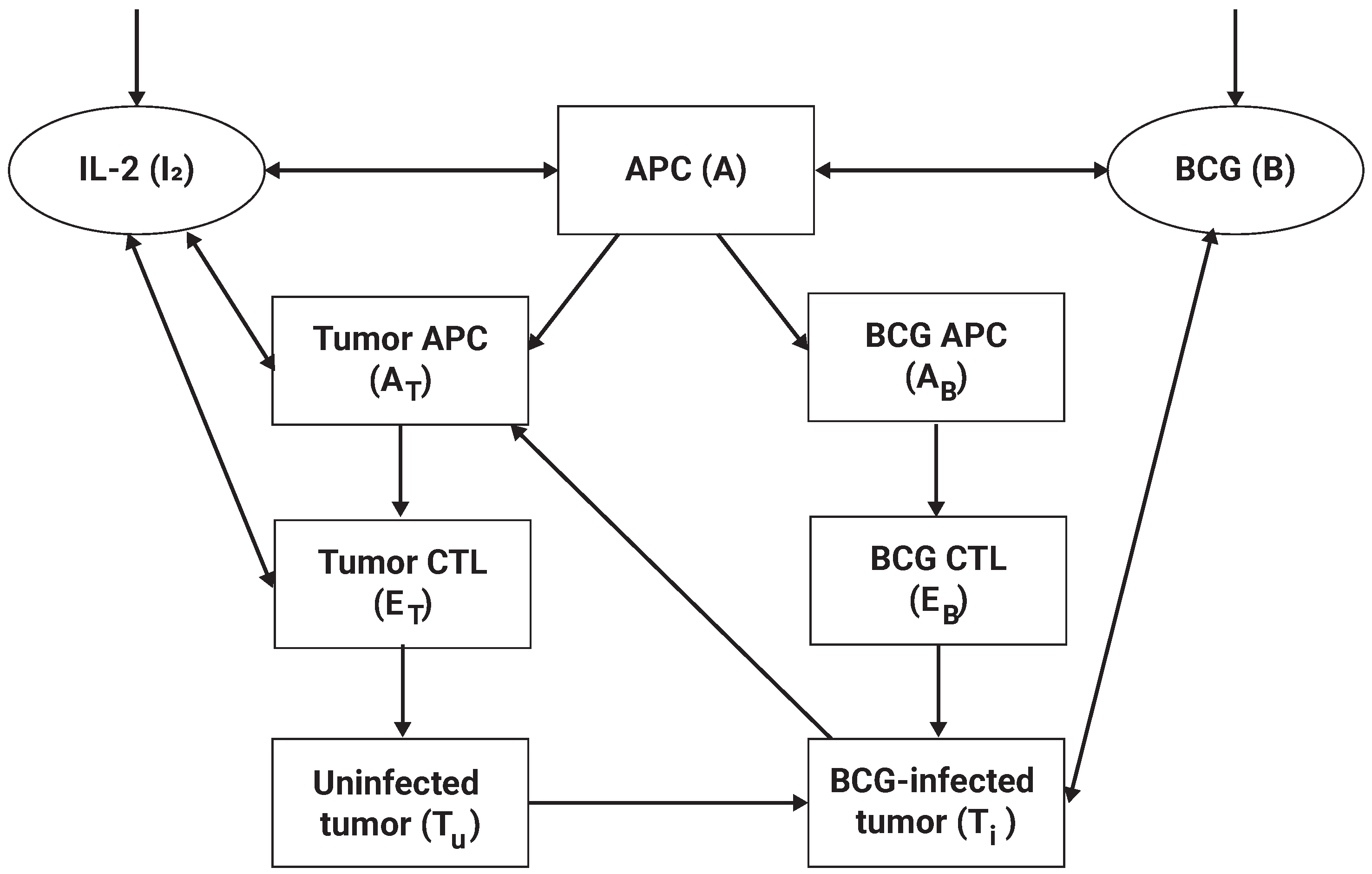
2. Biological Model
3. Personalized BCG-Based Treatment Scheduling
4. Evaluation
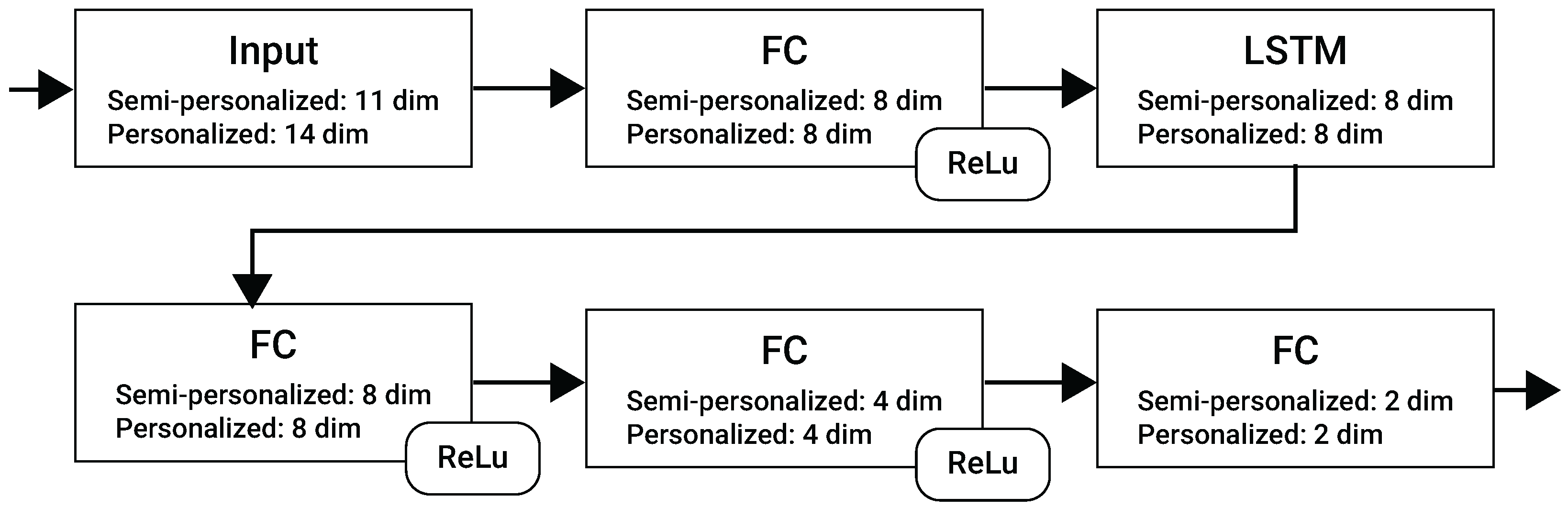
4.1. RNN Models
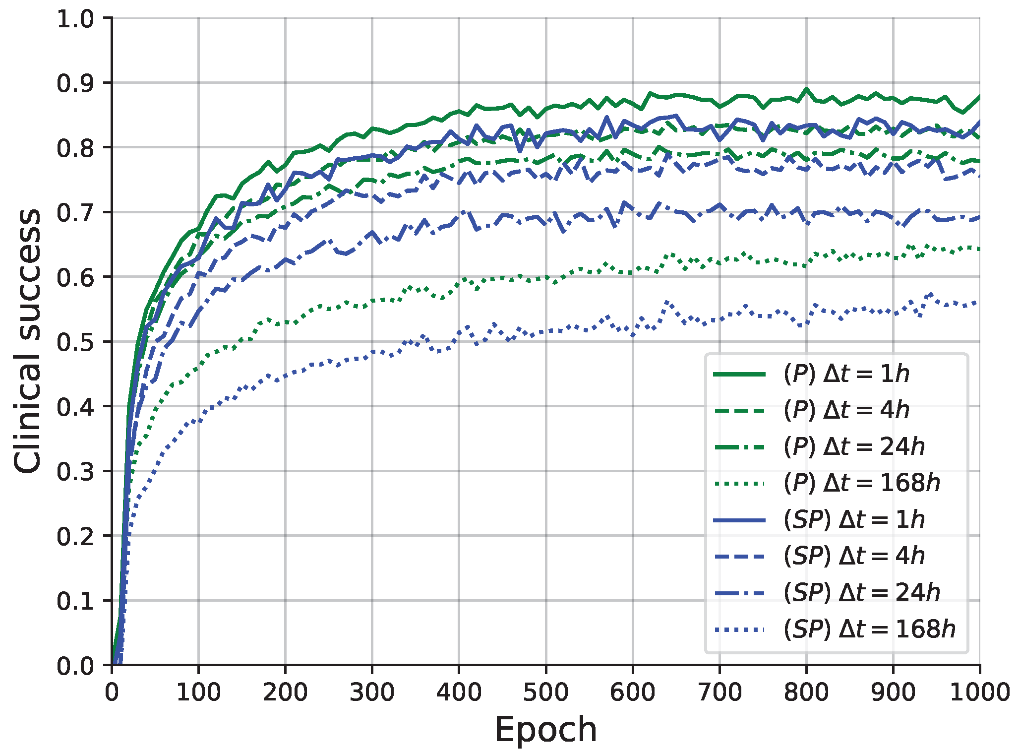
4.2. Learning Process
4.3. Comparison
4.4. Schedule Profiling
5. Discussion and Conclusions
Author Contributions
Funding
Data Availability Statement
Acknowledgments
Conflicts of Interest
References
- Cao, W.; Chen, H.D.; Yu, Y.W.; Li, N.; Chen, W.Q.; Ni, J. Changing profiles of cancer burden worldwide and in China: A secondary analysis of the global cancer statistics 2020. Chin. Med. J. 2021, 134, 783–791. [Google Scholar] [CrossRef] [PubMed]
- Weinberg, R.A. How Cancer Arises. Sci. Am. 1996, 275, 62–70. [Google Scholar] [CrossRef] [PubMed]
- Mohammadian, M.; Safari, A.; Bakeshei, K.A.; Bakeshei, F.A.; Asti, A.; Mohammadian-Hafshejani, A.; Salehiniya, H.; Emaiyan, M.; Khapour, H. Recent Patterns of Bladder Cancer Incidence and Mortality: A Global Overview. World Cancer Res. J. 2020, 7, e1464. [Google Scholar]
- Knowles, M.A. Molecular subtypes of bladder cancer: Jekyll and Hyde or chalk and cheese? Carcinogenesis 2006, 27, 361–373. [Google Scholar] [CrossRef] [PubMed] [Green Version]
- Shanock, L.R.; Baran, B.E.; Gentry, W.A.; Pattison, S.C.; Heggestad, E.D. Polynomial Regression with Response Surface Analysis: A Powerful Approach for Examining Moderation and Overcoming Limitations of Difference Scores. Discret. Contin. Dyn. Syst. Ser. B 2016, 1279–1295. [Google Scholar]
- Urdaneta, G.; Solsona, E.; Palou, J. Intravesical chemotherapy and BCG for the treatment of bladder cancer: Evidence and opinion. Eur. Urol. Suppl. 2008, 7, 542–547. [Google Scholar] [CrossRef]
- Morales, A.; Eidinger, D.; Bruce, A. Intracavity Bacillus Calmette-Guérin in the treatment of superficial bladder tumors. J. Urol. 1976, 116, 180–183. [Google Scholar] [CrossRef]
- Redelman-Sidi, G.; Glickman, M.S.; Bochner, B.H. The mechanism of action of BCG therapy for bladder cancer—A current perspective. Nat. Rev. Urol. 2014, 11, 153–162. [Google Scholar] [CrossRef]
- Herr, H.W.; Laudone, V.P.; Badalament, R.A.; Oettgen, H.F.; Sogani, P.C.; Freedman, B.D.; Melamed, M.R.; Whitmore, W.F. Bacillus Calmette-Guérin therapy alters the progression of superficial bladder cancer. J. Clin. Oncol. 1988, 6, 1450–1455. [Google Scholar] [CrossRef]
- Anastasiadis, A.; de Reijke, T.M. Best practice in the treatment of nonmuscle invasive bladder cancer. Ther. Adv. Urol. 2012, 4, 13–32. [Google Scholar] [CrossRef] [Green Version]
- Lamm, D. Improving Patient Outcomes: Optimal BCG Treatment Regimen to Prevent Progression in Superficial Bladder Cance. Eur. Urol. Suppl. 2006, 5, 654–659. [Google Scholar] [CrossRef]
- Ylösmäki, E.; Fusciello, M.; Martins, B.; Feola, S.; Hamdan, F.; Chiaro, J.; Ylosmaki, L.; Vaughan, M.J.; Viitala, T.; Kulkarni, P.S.; et al. Novel personalized cancer vaccine platform based on Bacillus Calmette-Guerin. J. Immunother. Cancer 2021, 9, e002707. [Google Scholar] [CrossRef] [PubMed]
- Bhattacharya, S.; Sah, P.P.; Banerjee, A.; Ray, S. Structural impact due to PPQEE deletion in multiple cancer associated protein - Integrin alpha: An In silico exploration. Biosystems 2020, 198, 104216. [Google Scholar] [CrossRef] [PubMed]
- Jordao, G.; Tavares, J.N. Mathematical models in cancer therapy. Biosystems 2017, 162, 12–23. [Google Scholar] [CrossRef] [PubMed]
- Hornberg, J.J.; Bruggeman, F.J.; Westerhoff, H.V.; Lankelma, J. Cancer: A Systems Biology disease. Biosystems 2006, 83, 81–90. [Google Scholar] [CrossRef] [PubMed]
- Chaplain, M.; Matzavinos, A. Mathematical Modelling of Spatio-temporal Phenomena in Tumour Immunology. In Tutorials in Mathematical Biosciences III: Cell Cycle, Proliferation, and Cancer; Friedman, A., Ed.; Springer: Berlin/Heidelberg, Germany, 2006; pp. 131–183. [Google Scholar]
- Ghaffari, A.; Naserifar, N. Optimal therapeutic protocols in cancer immunotherapy. Comput. Biol. Med. 2010, 40, 261–270. [Google Scholar] [CrossRef] [PubMed]
- Ahn, I.; Park, J. Drug scheduling of cancer chemotherapy based on natural actor-critic approach. Biosystems 2011, 106, 121–129. [Google Scholar] [CrossRef] [PubMed]
- Peter, J.; Schaal, S. Natural Actor-Critic. Neurocomputing 2008, 71, 1180–1190. [Google Scholar] [CrossRef]
- De Pillis, L.G.; Radunskaya, A. The dynamics of an optimally controlled tumor model: A case study. Math. Comput. Model. 2003, 37, 1221–1244. [Google Scholar] [CrossRef]
- Bazrafshan, N.; Lotfi, M.M. A finite-horizon Markov decision process model for cancer chemotherapy treatment planning: An application to sequential treatment decision making in clinical trials. Ann. Oper. Res. 2020, 295, 483–502. [Google Scholar] [CrossRef]
- Guzev, E.; Halachmi, S.; Bunimovich-Mendrazitsky, S. Additional Extension of the Mathematical Model for BCG Immunotherapy of Bladder Cancer and Its Validation by Auxiliary Tool. Int. J. Nonlinear Sci. Numer. Simul. 2019, 20, 675–689. [Google Scholar] [CrossRef]
- Shaikhet, L.; Bunimovich-Mendrazitsky, S. Stability analysis of delayed immune response BCG infection in bladder cancer treatment model by stochastic perturbations. Comput. Math. Methods Med. 2018, 2018, 9653873. [Google Scholar] [CrossRef] [PubMed]
- Lazebnik, T.; Bunimovich-Mendrazitsky, S. Improved Geometric Configuration for the Bladder Cancer BCG-Based Immunotherapy Treatment Model. In Proceedings of the Mathematical and Computational Oncology: Third International Symposium, ISMCO 2021, Virtual Event, 11–13 October 2021; Bebis, G., Gaasterland, T., Kato, M., Kohandel, M., Wilkie, K., Eds.; Springer: Berlin/Heidelberg, Germany, 2021; Volume 13060. [Google Scholar]
- Rentsch, C.A.; Biot, C.; Gsponer, J.R.; Bachmann, A.; Albert, M.L.; Breban, R. BCG-Mediated Bladder Cancer Immunotherapy: Identifying Determinants of Treatment Response Using a Calibrated Mathematical Model. PLoS ONE 2013, 8, e56327. [Google Scholar] [CrossRef] [PubMed]
- Starkov, K.E.; Bunimovich-Mendrazitsky, S. Dynamical properties and tumor clearance conditions for a nine-dimensional model of bladder cancer immunotherapy. Am. Inst. Math. Sci. 2016, 13, 1059–1075. [Google Scholar] [CrossRef] [PubMed] [Green Version]
- Bunimovich-Mendrazitsky, S.; Halachmi, S.S.; Kronik, N. Improving Bacillus Calmette Guerin (BCG) immunotherapy for bladder cancer by adding interleukin-2 (IL-2): A mathematical model. Math. Med. Biol. 2015, 33, 159–188. [Google Scholar]
- Song, D.; Powles, T.; Shi, L.; Zhang, L.; Ingersol, M.A.; Lu, Y.J. Bladder cancer, a unique model to understand cancer immunity and develop immunotherapy approaches. J. Pathol. 2019, 249, 151–165. [Google Scholar] [CrossRef] [Green Version]
- Bunimovich-Mendrazitsky, S.; Pisarev, V.; Kashdan, E. Modeling and simulation of a low-grade urinary bladder carcinoma. Comput. Biol. Med. 2014, 58, 118–129. [Google Scholar] [CrossRef]
- Bunimovich-Mendrazitsky, S.; Goltser, Y. Use of quasi-normal form to examine stability of tumor-free equilibrium in a mathematical model of BCG treatment of bladder cancer. Math. Biosci. Eng. 2011, 8, 529–547. [Google Scholar]
- Eikenberry, S.; Thalhauser, C.; Kuang, Y. Tumor-immune interaction, surgical treatment, and cancer recurrence in a mathematical model of melanoma. PLoS Comput. Biol. 2009, e1000362. [Google Scholar] [CrossRef] [Green Version]
- Lazebnik, T.; Bunimovich-Mendrazitsky, S.; Haroni, N. PDE Based Geometry Model for BCG Immunotherapy of Bladder Cancer. Biosystems 2021, 200, 104319. [Google Scholar] [CrossRef]
- Matzavinos, A.; Chaplain, M.A.; Kuznetsov, V.A. Mathematical modelling of the spatio-temporal response of cytotoxic T-lymphocytes to a solid tumour. Math. Med. Biol. 2004, 21, 1–34. [Google Scholar] [CrossRef] [PubMed]
- Guallar-Garrido, S.; Julián, E. Bacillus Calmette-Guerin (BCG) Therapy for Bladder Cancer: An Update. Immunotargets Ther. 2020, 13, 1–11. [Google Scholar] [CrossRef] [PubMed] [Green Version]
- Sanli, O.; Dobruch, J.; Knowles, M.A.; Burger, M.; Alemozaffar, M.; Nielsen, M.E.; Lotan, Y. Bladder cancer. Nat. Rev. Dis. Primers 2017, 17022. [Google Scholar] [CrossRef] [PubMed] [Green Version]
- Bunimovich-Mendrazitsky, S.; Byrne, H.; Stone, L. Mathematical Model of Pulsed Immunotherapy for Superficial Bladder Cancer. Bull. Math. Biol. 2008, 70, 2055–2076. [Google Scholar] [CrossRef] [PubMed]
- Shah, P.; Kendall, F.; Khozin, S.; Goosen, R.; Hu, J.; Laramie, J.; Ringel, M.; Schork, N. Artificial intelligence and machine learning in clinical development: A translational perspective. Npj Digit. Med. 2019, 2, 69. [Google Scholar] [CrossRef] [Green Version]
- Ngiam, K.Y.; Khor, I.W. Big data and machine learning algorithms for health-care delivery. Lancet Oncol. 2019, 20, e262–e273. [Google Scholar] [CrossRef] [PubMed]
- Colic, S.; Wither, R.G.; Lang, M.; Zhang, L.; Eubanks, J.H.; Bardakjian, B.L. Prediction of antiepileptic drug treatment outcomes using machine learning. J. Neural Eng. 2016, 14, 016002. [Google Scholar] [CrossRef] [PubMed] [Green Version]
- Kleinerman, A.; Rosenfeld, A.; Rosemarin, H. Machine-learning based routing of callers in an Israeli mental health hotline. Isr. J. Health Policy Res. 2022, 11, 1–15. [Google Scholar] [CrossRef]
- Rosemarin, H.; Rosenfeld, A.; Lapp, S.; Kraus, S. LBA: Online Learning-Based Assignment of Patients to Medical Professionals. Sensors 2021, 21, 3021. [Google Scholar] [CrossRef]
- Lim, B. Forecasting Treatment Responses Over Time Using Recurrent Marginal Structural Networks. In Proceedings of the Advances in Neural Information Processing Systems, Montreal, QC, Canada, 3–8 December 2018; Volume 31. [Google Scholar]
- Poulos, J.; Zeng, S. RNN-based counterfactual prediction, with an application to homestead policy and public schooling. J. R. Stat. Soc. Ser. C 2021, 70, 1124–1139. [Google Scholar] [CrossRef]
- Wang, L.; Tang, R.; He, X.; He, X. Hierarchical Imitation Learning via Subgoal Representation Learning for Dynamic Treatment Recommendation. In Proceedings of the Fifteenth ACM International Conference on Web Search and Data Mining, Tempe, AZ, USA, 21–25 February 2022; pp. 1081–1089. [Google Scholar]
- Jin, H.; Song, Q.; Hu, X. Auto-Keras: An Efficient Neural Architecture Search System. In Proceedings of the 25th ACM SIGKDD International Conference on Knowledge Discovery & Data Mining, Anchorage, AK, USA, 4–8 August 2019; pp. 1946–1956. [Google Scholar]
- Waring, J.; Lindvall, C.; Umeton, R. Automated machine learning: Review of the state-of-the-art and opportunities for healthcare. Artif. Intell. Med. 2020, 104, 101822. [Google Scholar] [CrossRef] [PubMed]
- Skeel, R.D.; Berzins, M. A Method for the Spatial Discretization of Parabolic Equations in One Space Variable. IAM J. Sci. Stat. Comput. 1990, 11, 1–32. [Google Scholar] [CrossRef]
- Lazebnik, T.; Yanetz, S.; Bunimovich-Mendrazitsky, S.; Haroni, N. Treatment of Bladder Cancer Using BCG Immunotherapy: PDE Modeling. Partial. Differ. Equations 2020, 26, 203–219. [Google Scholar]
- Lazebnik, T. Cell-Level Spatio-Temporal Model for a Bacillus Calmette–Guérin-Based Immunotherapy Treatment Protocol of Superficial Bladder Cancer. Cells 2022, 15, 2372. [Google Scholar] [CrossRef]
- Samek, W.; Montavon, G.; Lapuschkin, S.; Anders, C.J.; Müller, K.R. Explaining Deep Neural Networks and Beyond: A Review of Methods and Applications. Proc. IEEE 2021, 109, 247–278. [Google Scholar] [CrossRef]
- Gulum, M.A.; Trombley, C.M.; Kantardzic, M. A Review of Explainable Deep Learning Cancer Detection Models in Medical Imaging. Appl. Sci. 2021, 11, 4573. [Google Scholar] [CrossRef]
- Bai, X.; Wang, X.; Liu, X.; Liu, Q.; Song, J.; Sebe, N.; Kim, B. Explainable deep learning for efficient and robust pattern recognition: A survey of recent developments. Pattern Recognit. 2021, 120, 108102. [Google Scholar] [CrossRef]
- Veturi, Y.A.; Woof, W.; Lazebnik, T.; Moghul, I.; Wagner, S.K.; de Guimarães, T.A.C.; Daich Varela, M.; Patel, P.J.; Beck, S.; Webster, A.R.; et al. SynthEye: Investigating the Impact of Synthetic Data on Artificial Intelligence-assisted Gene Diagnosis of Inherited Retinal Disease. Ophthalmol. Sci. 2023, 3, 100258. [Google Scholar] [CrossRef]
- Lazebnik, T.; Bahouth, Z.; Bunimovich-Mendrazitsky, S.; Halachmi, S. Predicting acute kidney injury following open partial nephrectomy treatment using SAT-pruned explainable machine learning model. BMC Med. Inform. Decis. Mak. 2022, 22, 133. [Google Scholar] [CrossRef]
- Rosenfeld, A.; Benrimoh, D.; Armstrong, C.; Mirchi, N.; Langlois-Therrien, T.; Rollins, C.; Tanguay-Sela, M.; Mehltretter, J.; Fratila, R.; Israel, S.; et al. Big Data analytics and artificial intelligence in mental healthcare. In Applications of Big Data in Healthcare; Elsevier: Amsterdam, The Netherlands, 2021; pp. 137–171. [Google Scholar]


| Parameter | Description | Average Value |
|---|---|---|
| APC half life () | ||
| Activated APC half life () | ||
| Effector cells mortality rate W/O IL-2 () | ||
| Effector cells mortality rate IL-2 () | 0.034 | |
| BCG half life () | 0.1 | |
| The rate of BCG binding with APC () | ||
| Infection rate of tumor cells by BCG () | ||
| Rate of E deactivation after binding with infected tumor cells () | ||
| Rate of destruction of infected tumor cells by effector cells () | ||
| Production rate of TAA-APC () | ||
| Recruitment rate of effector cells in response to signals released by BCG-infected and activated APC () | ||
| Recruitment rate of effector cells in response to signals released by TAA-infected and activated APC () | ||
| Initial APC cell numbers () | ||
| Rate of recruited additional resting APCs () | ||
| r | Tumor growth rate () | |
| b | Bio-effective dose of BCG | |
| Migration rate of TAA-APC and bacteria activated APC to the lymph node () | ||
| Efficacy of an effector cell on tumor cell () | ||
| g | Michaelis–Menten constant for BCG activated CTLs and for TAA-CTLs () | |
| Michaelis–Menten constant for tumor cells () | ||
| K | Maximal tumor cell population () | |
| Rate of IL-2 production IU () | ||
| The proportion of IL-2 used for differentiation of effector cells IU () | ||
| Degradation rate () | ||
| Recruitment rate of Tumor-Ag-activated APC cells in response to signals released after binding effector cells, that react to BCG infection, with infected tumor cells () | ||
| The release term per tumor cell () | ||
| Michaelis-Menten saturation dynamics (1) | ||
| Michaelis constant (1) | ||
| The constant rate, accounts for degradation of () | ||
| Michaelis–Menten constant for IL-2 () | 10,000 | |
| Rate of external source (1) |
| Objective Configuration | Model | Cancer Cell Population | Administered BCG | Administered IL-2 | ISR | Clinical Success |
|---|---|---|---|---|---|---|
| Baseline [7] | ||||||
| Guzev et al. [22] | ( | |||||
| Semi-personalized RNN | ||||||
| Personalized RNN | ||||||
| Baseline [7] | ||||||
| Guzev et al. [22] | ||||||
| Semi-personalized RNN | ||||||
| Personalized RNN | ||||||
| Baseline [7] | ||||||
| Guzev et al. [22] | ||||||
| Semi-personalized RNN | ||||||
| Personalized RNN |
Disclaimer/Publisher’s Note: The statements, opinions and data contained in all publications are solely those of the individual author(s) and contributor(s) and not of MDPI and/or the editor(s). MDPI and/or the editor(s) disclaim responsibility for any injury to people or property resulting from any ideas, methods, instructions or products referred to in the content. |
© 2023 by the authors. Licensee MDPI, Basel, Switzerland. This article is an open access article distributed under the terms and conditions of the Creative Commons Attribution (CC BY) license (https://creativecommons.org/licenses/by/4.0/).
Share and Cite
Yaniv-Rosenfeld, A.; Savchenko, E.; Rosenfeld, A.; Lazebnik, T. Scheduling BCG and IL-2 Injections for Bladder Cancer Immunotherapy Treatment. Mathematics 2023, 11, 1192. https://doi.org/10.3390/math11051192
Yaniv-Rosenfeld A, Savchenko E, Rosenfeld A, Lazebnik T. Scheduling BCG and IL-2 Injections for Bladder Cancer Immunotherapy Treatment. Mathematics. 2023; 11(5):1192. https://doi.org/10.3390/math11051192
Chicago/Turabian StyleYaniv-Rosenfeld, Amit, Elizaveta Savchenko, Ariel Rosenfeld, and Teddy Lazebnik. 2023. "Scheduling BCG and IL-2 Injections for Bladder Cancer Immunotherapy Treatment" Mathematics 11, no. 5: 1192. https://doi.org/10.3390/math11051192