Hybrid GPU–CPU Efficient Implementation of a Parallel Numerical Algorithm for Solving the Cauchy Problem for a Nonlinear Differential Riccati Equation of Fractional Variable Order

Abstract

The numerical solution for fractional dynamics problems can create a high computational load, which makes it necessary to implement efficient algorithms for their solution. The main contribution to the computational load of such computations is created by heredity (memory), which is determined by the dependence of the current value of the solution function on previous values in the time interval. In terms of mathematics, the heredity here is described using a fractional differentiation operator in the Gerasimov–Caputo sense of variable order. As an example, we consider the Cauchy problem for the non-linear fractional Riccati equation with non-constant coefficients. An efficient parallel implementation algorithm has been proposed for the known sequential non-local explicit finite-difference numerical solution scheme. This implementation of the algorithm is a hybrid one, since it uses both GPU and CPU computational nodes. The program code of the parallel implementation of the algorithm is described in C and CUDA C languages, and is developed using OpenMP and CUDA hardware, as well as software architectures. This paper presents a study on the computational efficiency of the proposed parallel algorithm based on data from a series of computational experiments that were obtained using a computing server NVIDIA DGX STATION. The average computation time is analyzed in terms of the following: running time, acceleration, efficiency, and the cost of the algorithm. As a result, it is shown on test examples that the hybrid version of the numerical algorithm can give a significant performance increase of 3–5 times in comparison with both the sequential version of the algorithm and OpenMP implementation.

1. Introduction

The fractional differentiation operator is a generalization of the concept of derivative, to the case of non-integer order of differentiation.This direction originated almost immediately after the appearance of integro-differential calculus about 300 years ago [1]. The study of this topic continues in the current day, and is associated with such names as Uchaikin V. [2], Psxy A. [3], Kilbas A. [4,5], Ortigueira M. D. [6,7], Patnaik S. [8], and many others. You can learn more about the history of the origins of fractional differential calculus in the excellent encyclopedia written by Samko S., Kilbas A., and Marichev O. on such a complex topic as “Integrals and derivatives of fractional order and some of their applications” [4].

The fractional calculus is closely related to the theory of fractals, which is reflected in the works of [9]. In particular, there is a connection between the fractal (Hausdorff) dimension of the medium and the orders of fractional operators. This is related to the concept of heredity—the property of a system or process to retain a memory of its past. The concept of heredity is equivalent to such concepts as consequence, heredity, residuality, memory, and lag, as well as non-locality, which was first introduced in the paper [10] by the Italian mathematician Vito Volterra in 1912. The property of hereditariness can be possessed by such systems in which not only the current state of the system, i.e., the initial values of the state parameters of the system and some time derivatives, but also a finite number of previous states of the system [2] are taken into account. Such models are called non-local in time [11]. There exist today various definitions regarding the meaning of the fractional differentiation operator: Liouville, Riemann–Liouville, Weyl, Grunwald–Letnikov, and many others. And for some of them, there are even more generalizations to the case of the VO (variable order) of order [7,8], which in turn leads to variable non-locality.

As a consequence, the applications of fractional-differential calculus in various branches of science and engineering are increasingly being developed [12,13]. The generalization of known applications and the development of new mathematical models that take into account the hereditary function allows one to clarify known results. Today, the derivatives and integrals of non-integer orders are already successfully used in many areas of science and technology. For example this in found in the following: economics [14,15]; physics and mechanics [16]; hydrodynamic modeling [17]; meteorology and diffusion [18]; modeling complex acoustic oscillations [19]; viscoelastic waves [20]; and many other fields of science.

Attempts to describe such processes in terms of fractional dynamics give rise to rather complicated model integro-differential equations and systems of equations, which often have to be solved numerically. Even if the proposed numerical scheme is relatively simple, it is usually the approximation of the fractional differentiation or integration operator [21] that starts to create difficulties, which inevitably increases the computational complexity of the numerical scheme. In mathematical modeling that is based on ODEs and PDEs, in some cases, it is possible to use sequential algorithms that implement numerical solution schemes and obtain results in an acceptable time. However, when generalizing these models to using fractional calculus, the computation time can increase dramatically due to memory or non-locality effects. It is then expedient to use parallel algorithms of a numerical solution that is realized both on the CPU and GPU nodes of computing systems to accelerate the calculations in those parts of the numerical scheme where possible.

For example, the papers [22,23] investigate the issues of computational acceleration in modeling some diffusion processes that are not based on the fractional Gerasimov–Caputo derivative [24,25], which is non-local to spatial variables. The authors Bogaenko V.A. and Bulavatskiy V.M. proposed to reduce the computational accuracy at the stage of building the approximation of the fractional Gerasimov–Caputo derivative for acceleration. It was proposed to solve the model equation numerically by using finite-difference schemes. The proposed schemes were implemented as parallel algorithms for systems with distributed memory and GPUs (graphics acceleration units). It is shown that by using such approaches it is possible to speed up computations by several times via proposed mathematical model.

The literature review shows that there are no studies devoted to the development of parallel algorithms for solving the Cauchy problem for nonlinear fractional equations with Gerasimov–CaputoVO. In particular, the realization of hybrid algorithms of a parallel explicit finite-difference scheme for solving the fractional Riccati equation on both CPU and GPU nodes of a computing system have not been investigated; thus, this will be the subject of this paper.

The research plan of the article is as follows: Section 2 describes the hardware base and principles of the organization of parallel computing, for which the proposed efficient parallel algorithm of numerical solution is developed; Section 3 gives the formulation of the Cauchy problem for the nonlinear equation with a fractional derivative of the Gerasimov–Caputo VO. In particular, the fractional Riccati equation is considered. A non-local explicit finite-difference scheme for the numerical solution of the problem is given; Section 4, in the form of code blocks of the C programming language, describes a hybrid parallel algorithm that realizes the explicit numerical scheme. The whole code located in the blocks represents a complete function implementing the numerical scheme; and Section 5 analyzes the efficiency of the presented hybrid parallel algorithm of the explicit finite-difference scheme in comparison with its best sequential version.

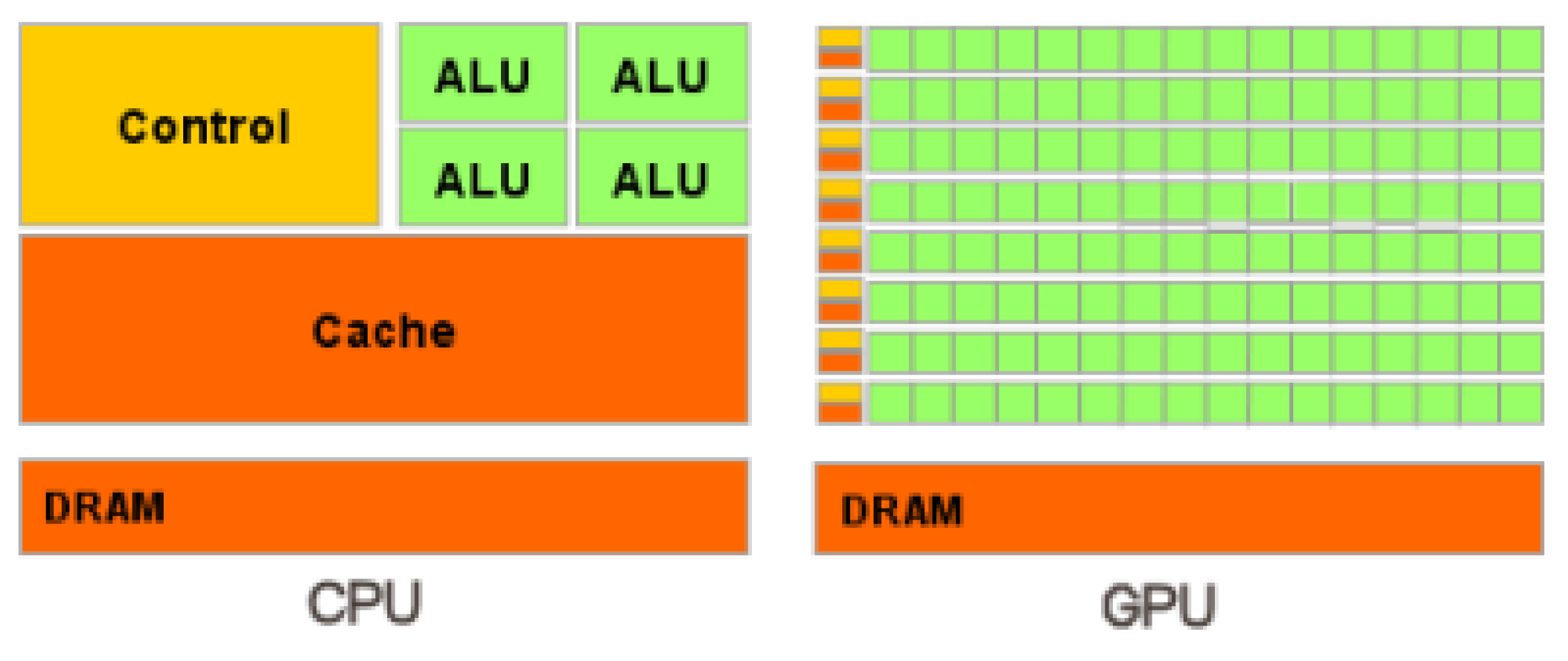
2. About Organization of Parallel Computations on CPU and GPU Nodes of a Computing System

It is difficult to overestimate how much computing technology and devices have infiltrated our lives, the most notable of which is computers. The basis of any computer or computing system is the central processing unit (CPU), which executes program instructions and coordinates all other nodes of the computing system [26]. The main part of the CPU is the core—a collection of data buses and caches, control units, and arithmetic-logic units (ALUs) [26]. For the last 20 years, the never-ending race has taken CPU architecture to a new level—multi-core. Within such CPUs there are physical cores—specific hardware blocks and logical cores—that are independent threads to which the CPU is able to distribute program instructions (code) [27]. Then, a specially designed program—a parallel algorithm—can be executed on such a computational node.

To solve the problems of developing parallel numerical algorithms, one of the technologies chosen is OpenMP—an open standard software interface for parallel systems with CPUs and their shared memory [28]. OpenMP implements parallel computing by using the idea of multithreading—multiple CPU threads running tasks in parallel. This is achieved by providing the developer with a set of directives for compilers, function libraries, and environment variables. The high-level language C was chosen as the main programming language because of its versatility and rather large freedom of working with memory [29]. And also because OpenMP is officially supported by C and the C++ programming languages.

The ideas of code development taking into account CPU multithreading are also applicable to GPUs. Their main difference is that while CPUs can solve several complex tasks in parallel, GPUs are oriented to the execution of programs with a large amount of single-type arithmetic operations. This way of organizing parallel calculations is called single instruction multiple data (SIMD) [26], i.e., when several processors perform the same operation simultaneously but on different data. From Figure 1, we can see that the CPU has a system of CPU caches and complex ALUs, while the GPU contains many simplified ALUs that share a common memory.

GPU memory is hierarchically structured and optimized for maximum bandwidth. And to achieve the best acceleration from the developed parallel algorithms on GPUs, it is necessary to think over the memory access of the program code and also to take into account the hardware features. All this allows one to improve performance in these kinds of computational tasks, but it makes programming more difficult [30].

The tool for working with GPUs in this article will be NVIDIA’s hardware and software parallel computing architecture for GPUs. This is also called Compute Unified Device Architecture (CUDA), and it allows us to significantly increase computational performance. CUDA gives you the ability to control the RAM of the GPU at will, and it generally provides a wide range of tools. The architecture invites us to implement functions executable on a GPU, also called a device, using addons of the C programming language, which are called CUDA C. In turn, we will name the CPU as host, thus separating the code executable on CPU and GPU [30]. We also note that the high-level programming language C has versatility and quite a lot of freedom of working with memory [29], which is very useful for designing efficient algorithms.

The ideas that led to the creation of the CUDA hardware-software architecture are somewhat similar to the ideas of the OpenMP software standard [28]. In particular, this is achieved in simplifying and bringing to a single standard the work with computing equipment, and providing a convenient program interface to developers, thereby solving the problems that arose earlier at the stage of «non-graphical» calculations on GPU. For more details, see [30] (p. 5).

In the problem we are considering, there is a need to utilize a supercomputer and its computing power [31,32]. The main reason is the ability to run simulations with an extremely small h sampling step. Since the amount of RAM memory that supercomputer technologies can provide us with allows us to operate on matrices and vectors with large dimensions, it allows us to concentrate on the organization of the efficient loading of CPUs and GPUs with calculations, while the software implementation of parallel algorithms of numerical solution schemes is provided.

3. Mathematical Problem Statement

There are many tens of definitions for the fractional differentiation operator, but we will focus on applying one of them [33]. We consider, in this paper, the communication of the Gerasimov–Caputo fractional differentiation operator [24,25], which is non-local in time $0<\alpha <1$, to the Gerasimov–Caputo VO, where $0<\alpha \left(t\right)<1$—i.e., the non-constant order of the fractional derivative. This generalization is studied in detail in the works of the author Tverdyi D.A. [34,35] and has the following form:

$${\partial }_{0t}^{\alpha \left(t\right)}u\left(\sigma \right)=\frac{1}{\mathrm{\Gamma }(1-\alpha (t\left)\right)}{\int }_0^t\frac{\dot{u}\left(\sigma \right)}{{(t-\sigma )}^{\alpha \left(t\right)}}d\sigma ,$$

(1)

where $u\left(t\right)\in C[0,T]$ is the one-dimensional local in a space solution function; the derivative $\dot{u}\left(t\right)=\frac{du}{dt}$; $t\in [0,T]$ is the current simulation time; $T>0$ is the total simulation time; and $\mathrm{\Gamma }(.)$ is the Euler gamma function, which monotonically decreases on the interval $0<x<1$.

Definition 1. 

The introduction of such (1) generalizations with variable nonlocality allows a more accurate description of the time series of some dynamical processes with memory [36,37,38].

The concept of heredity was proposed and studied by the Italian mathematician Vito Volterra [11]. In the [2] paper, various physical processes with hereditary effects were investigated. We will not elaborate on the theoretical aspects related to the description of heredity (memory effect) using fractional derivatives.

In the following section, for the sake of an example, we consider a more specific kind of model equation; namely, the Riccati equation [39] when it is in its fractional analog, for which the Cauchy problem will be of the form:

$${\partial }_{0t}^{\alpha \left(t\right)}u\left(\sigma \right)+a\left(t\right)u^2\left(t\right)-b\left(t\right)u\left(t\right)-c\left(t\right)=0,u\left(0\right)=u_0,$$

(2)

where $u\left(t\right)\in C^2[0,T]$—the unknown solution function; $a\left(t\right)$, $b\left(t\right)$, $c\left(t\right)$$\in C[0,T]$—the set functions determining the values of the coefficients at each moment of time.

Remark 1. 

However, for example, in [34], we consider a generalized form of a nonlinear fractional Equation (2) for which a local Cauchy problem with variable time nonlocality is posed [5] due to the use of the VO operator (1). Such a problem can describe a wide class of dynamic processes with variable memory in saturated environments [40].

Remark 2. 

The model (2) presented above, also called the heredity $\alpha \left(t\right)$-model, is used by the authors in the problems of the emanation of radon gas [41] through porous media, where the order of the fractional derivative can be responsible for the intensity of the transport process ${}^{222}$Rn, which is related to the permeability of the geo-environment: porosity, fracturing, etc. [2].

We will solve this problem (2) numerically using the methods of finite-difference schemes for solutions of differential equations, and the Gerasimov–Caputo VO approximation (1) is introduced according to the [34,35]. This manuscript implements a relatively simple non-local explicit finite-difference scheme (EFDS) that was composed by Euler’s method [42]. However, there is a difficulty in deriving a discrete analog (approximation) of the fractional Gerasimov–Caputo derivative VO (1) with this scheme.

To obtain the numerical solution of [34,43], according to Euler’s method, it can be represented as a finite-difference scheme of the form:

$$\begin{array}{c}\hfill \begin{array}{c}{u}_1=\frac{1}{A_0}\left(\left(A_0(1-w_1^0)+b_0\right)u_0-a_0{u}_0^2+c_0\right),\\ u_2=\frac{1}{A_1}\left(\left(A_1\left(1-w_1^1\right)+b_1\right)u_1+A_1{w}_1^1{u}_0-a_1{u}_1^2+c_1\right),\\ u_{i+1}=\frac{1}{A_i}\left[\left(A_i\left(1-w_1^i\right)+b_i\right)u_i+A_i{w}_1^i{u}_{i-1}-\right.\\ \left.A_i{\displaystyle \sum _{j=2}^i}{w}_j^i\left(u_{i-j+1}-u_{i-j}\right)-a_i{u}_i^2+b_i{u}_i+c_i\right],\\ A_i=\frac{h^{-{\alpha }_{i+1}}}{\mathrm{\Gamma }(2-{\alpha }_{i+1})},w_j^i={(j+1)}^{1-{\alpha }_{i+1}}-j^{1-{\alpha }_{i+1}},w_1^i={\displaystyle \sum _{i=0}^{N-1}}\left(2^{1-{\alpha }_{i+1}}-1^{1-{\alpha }_{i+1}}\right),\end{array}\end{array}$$

(3)

where $u_0=C$ is the initial condition of the Cauchy problem (2); C is a known constant; $h=T/N$ is the uniform grid discretization step; N is the number of grid nodes; and $i=2,\dots ,N-1$ is the node number of the computational grid.

In [34] (p. 14), the convergence and stability of EFDS (3) are investigated. It is shown that EFDS (3) is stable and converges to order $O\left(h\right)$ under the condition:

$$h\le {\displaystyle \frac{2^{{\displaystyle 1-\underset{i}{max}\left({\alpha }_i\right)}}-1}{{\displaystyle \underset{i}{max}\left(b_i\right)}}}.$$

(4)

Remark 3. 

In this paper, the numerical scheme (3) slightly differs from the one presented in [34] (p. 14) in that in (3) there appears a weighting factor $w_1^i$ that is derived from the factor $w_j^i$ in order to speed up the computation. This does not impact the accuracy of EFDS (3) computation, convergence, and stability.

4. Software Implementation of the Hybrid EFDS Algorithm

Let us consider step by step an efficient hybrid parallel program implementation of EFDS (3). We will provide the code listing, which is broken into parts for the necessary explanations.

Remark 4. 

The structures (see Listings 1–3), functions (see Listings 4 and 5), and directives (see Listing 6) described in this chapter must be declared before declaring the code for a method function (see Listings 7–19). From the code snippets (see Listings 7–19), we can compose a function  EFDS_parallel_HYBRID()  that works and is debugged. The function code assumes a GPU function call (see Listings 20 and 21) necessary for the calculations.

Listing 1. Data type INP_PAR—modeling input parameters.

typedef struct input {     int   T;                        //  time of numerical experement.     int   N;                        //  number cells of grid (lattice).     float u_0;                      //  start point, for Cauchy poblem.     char  type_method[CHAR_LEN];    //= EFDS \ IFDS     char  type_algorithm[CHAR_LEN]; //= sequential \ parallel(OpenMP)                                     //  parallel(HYBRID)     int   num_threads_CPU;          //  num threads parallel (OpenMP)     int   num_threads_GPU;          //  num threads parallel (CUDA),     char  num_GPU_using[CHAR_LEN];  //  num GPU device : best GPU     char  current_method[CHAR_LEN]; //= EFDS \ IFDS } INP_PAR;

Listing 1. Data type INP_PAR—modeling input parameters.

typedef struct input {     int   T;                        //  time of numerical experement.     int   N;                        //  number cells of grid (lattice).     float u_0;                      //  start point, for Cauchy poblem.     char  type_method[CHAR_LEN];    //= EFDS \ IFDS     char  type_algorithm[CHAR_LEN]; //= sequential \ parallel(OpenMP)                                     //  parallel(HYBRID)     int   num_threads_CPU;          //  num threads parallel (OpenMP)     int   num_threads_GPU;          //  num threads parallel (CUDA),     char  num_GPU_using[CHAR_LEN];  //  num GPU device : best GPU     char  current_method[CHAR_LEN]; //= EFDS \ IFDS } INP_PAR;

Listing 2. Data type OUT_RES– modeling results and output parameters.

typedef struct output {     int   T;     int   N;     float u_0;     char  type_method[CHAR_LEN];     char  type_algorithm[CHAR_LEN];     int   num_threads_CPU;     int   num_threads_GPU;     char  num_GPU_using[CHAR_LEN];     float h; // step of discretisation.     float ∗res; // result calculation.     float mem_aloc_CPU; // value memory was allocated on CPU (RAM).     float mem_aloc_GPU; // value memory was allocated for GPU (DRAM). } OUT_RES;

Listing 2. Data type OUT_RES– modeling results and output parameters.

typedef struct output {     int   T;     int   N;     float u_0;     char  type_method[CHAR_LEN];     char  type_algorithm[CHAR_LEN];     int   num_threads_CPU;     int   num_threads_GPU;     char  num_GPU_using[CHAR_LEN];     float h; // step of discretisation.     float ∗res; // result calculation.     float mem_aloc_CPU; // value memory was allocated on CPU (RAM).     float mem_aloc_GPU; // value memory was allocated for GPU (DRAM). } OUT_RES;

Listing 3. Data type MATC—information about location and time measurements, as well as the declaration of objects of this structure:

typedef struct mesure_all_times_calc {     float  time_calc_res_m_3;     struct timeval tv1, tv2, dtv;        char   location[CHAR_LEN];  // where fields MATC object was filled } MATC; MATC measure_PARA;  // FOR mesure time working Parallel part code MATC measure_SEQU;  // FOR mesure time working Sequenitial part code MATC measure_MAIN;  // FOR mesure time working All part’s code

Listing 3. Data type MATC—information about location and time measurements, as well as the declaration of objects of this structure:

typedef struct mesure_all_times_calc {     float  time_calc_res_m_3;     struct timeval tv1, tv2, dtv;        char   location[CHAR_LEN];  // where fields MATC object was filled } MATC; MATC measure_PARA;  // FOR mesure time working Parallel part code MATC measure_SEQU;  // FOR mesure time working Sequenitial part code MATC measure_MAIN;  // FOR mesure time working All part’s code

Listing 4. Function tic()—to start measuring time into MATC objects.

MATC tic( MATC measure ) {     gettimeofday( &measure.tv1, NULL );   // most accuracy method !     return measure; }

Listing 4. Function tic()—to start measuring time into MATC objects.

MATC tic( MATC measure ) {     gettimeofday( &measure.tv1, NULL );   // most accuracy method !     return measure; }

Listing 5. Function toc()—completing measurements and calculating elapsed time.

MATC toc( MATC measure ) {     gettimeofday( &measure.tv2, NULL );     measure.dtv.tv_sec  = measure.tv2.tv_sec  - measure.tv1.tv_sec;     measure.dtv.tv_usec = measure.tv2.tv_usec - measure.tv1.tv_usec;     if( measure.dtv.tv_usec < 0 ) {         measure.dtv.tv_sec--;         measure.dtv.tv_usec += 1000000;     }     float elapsed_dtv = measure.dtv.tv_sec ∗ 1000 +                         measure.dtv.tv_usec / 1000;     measure.time_calc_res_m_3 = (double)elapsed_dtv / 1000;     return measure; }

Listing 5. Function toc()—completing measurements and calculating elapsed time.

MATC toc( MATC measure ) {     gettimeofday( &measure.tv2, NULL );     measure.dtv.tv_sec  = measure.tv2.tv_sec  - measure.tv1.tv_sec;     measure.dtv.tv_usec = measure.tv2.tv_usec - measure.tv1.tv_usec;     if( measure.dtv.tv_usec < 0 ) {         measure.dtv.tv_sec--;         measure.dtv.tv_usec += 1000000;     }     float elapsed_dtv = measure.dtv.tv_sec ∗ 1000 +                         measure.dtv.tv_usec / 1000;     measure.time_calc_res_m_3 = (double)elapsed_dtv / 1000;     return measure; }

Listing 6. A few helper directives.

#define CHAR_LEN 256   // default num char elements ∗char[] massive     #define EPSILON 1e-2   // numerical methods accuracy     #define ZERO 0     #define def_min(a,b) (a<b?a:b)     #define def_max(a,b) (a>b?a:b)

Listing 6. A few helper directives.

#define CHAR_LEN 256   // default num char elements ∗char[] massive     #define EPSILON 1e-2   // numerical methods accuracy     #define ZERO 0     #define def_min(a,b) (a<b?a:b)     #define def_max(a,b) (a>b?a:b)

4.1. Code for Parallel EFDS Implementation

EFDS calculation by the algorithm using OpenMP and CUDA is performed by the function EFDS_parallel_HYBRID(), the only argument of which is an object of the class INP_PAR (see Listing 1), which is filled in with the help of the auxiliary function reading the necessary parameters from .txt of the user control file:

Listing 7. Startof the function that realizes the numerical scheme.

OUT_RES EFDS_parallel_HYBRID( INP_PAR input ) {     memcpy( input.current_method, (char ∗)"EFDS", CHAR_LEN );

Listing 7. Startof the function that realizes the numerical scheme.

OUT_RES EFDS_parallel_HYBRID( INP_PAR input ) {     memcpy( input.current_method, (char ∗)"EFDS", CHAR_LEN );

This function will be run within a short program complex, the whole code of which is not given in this article. However, some of its auxiliary functions necessary for the operation of EFDS_parallel_HYBRID() have been given above.

The allocation of RAM for the variables necessary in the process of calculation, both on CPU and GPU devices, for the convenience of orientation in the code is carried out at the beginning of the function body:

Listing 8. CPU RAM allocation.

int   T   = input.T;   //  time of numerical experement.     int   N   = input.N;   // number cells of grid (lattice).     float h   = (float)T / (float)N;  // step of discretisation.     float u_0 = input.u_0; // start point for Cauchy poblem.     OUT_RES     output;     int N_p1  = N + 1;     float    a[ N ];      // massive value ’a(t)’.     float    b[ N ];      // massive value ’b(t)’.     float    c[ N ];      // massive value ’c(t)’.     float alpha[ N_p1 ];   // massive value ’alpha(t)’     float    A[ N ];      // 1-st Weight coefficient ’A’     float   w_1[ N ];     float    u[ N_p1 ];   // solve. ( + 1 because u[0] include)     float summ_diff_u;     float ∗w;     w = (float∗) malloc( (N ∗ N) ∗ sizeof(float) );     float mem_aloc_CPU = sizeof u + sizeof a + sizeof b + sizeof c +                          sizeof alpha + sizeof A + sizeof w_1;     mem_aloc_CPU += (( (float)N ∗ (float)N ) ∗ 4); // sizeof w

Listing 8. CPU RAM allocation.

int   T   = input.T;   //  time of numerical experement.     int   N   = input.N;   // number cells of grid (lattice).     float h   = (float)T / (float)N;  // step of discretisation.     float u_0 = input.u_0; // start point for Cauchy poblem.     OUT_RES     output;     int N_p1  = N + 1;     float    a[ N ];      // massive value ’a(t)’.     float    b[ N ];      // massive value ’b(t)’.     float    c[ N ];      // massive value ’c(t)’.     float alpha[ N_p1 ];   // massive value ’alpha(t)’     float    A[ N ];      // 1-st Weight coefficient ’A’     float   w_1[ N ];     float    u[ N_p1 ];   // solve. ( + 1 because u[0] include)     float summ_diff_u;     float ∗w;     w = (float∗) malloc( (N ∗ N) ∗ sizeof(float) );     float mem_aloc_CPU = sizeof u + sizeof a + sizeof b + sizeof c +                          sizeof alpha + sizeof A + sizeof w_1;     mem_aloc_CPU += (( (float)N ∗ (float)N ) ∗ 4); // sizeof w

Listing 9. GPU RAM allocation.

float ∗dev_a;     cudaMalloc( (void∗∗)&dev_a,     N ∗ sizeof(float) );     float ∗dev_b;     cudaMalloc( (void∗∗)&dev_b,     N ∗ sizeof(float) );     float ∗dev_c;     cudaMalloc( (void∗∗)&dev_c,     N ∗ sizeof(float) );     float ∗dev_alpha;     cudaMalloc( (void∗∗)&dev_alpha, N_p1 ∗ sizeof(float) );     float ∗dev_A;     cudaMalloc( (void∗∗)&dev_A,     N ∗ sizeof(float) );     float ∗dev_w;     cudaMalloc( (void∗∗)&dev_w, (N ∗ N) ∗ sizeof(float) );     float ∗dev_w_1;     cudaMalloc( (void∗∗)&dev_w_1,   N ∗ sizeof(float) );     float mem_aloc_GPU = sizeof a + sizeof b + sizeof c+                          sizeof alpha + sizeof A + sizeof w_1;     mem_aloc_GPU += (( (float)N ∗ (float)N ) ∗ 4);// sizeof w

Listing 9. GPU RAM allocation.

float ∗dev_a;     cudaMalloc( (void∗∗)&dev_a,     N ∗ sizeof(float) );     float ∗dev_b;     cudaMalloc( (void∗∗)&dev_b,     N ∗ sizeof(float) );     float ∗dev_c;     cudaMalloc( (void∗∗)&dev_c,     N ∗ sizeof(float) );     float ∗dev_alpha;     cudaMalloc( (void∗∗)&dev_alpha, N_p1 ∗ sizeof(float) );     float ∗dev_A;     cudaMalloc( (void∗∗)&dev_A,     N ∗ sizeof(float) );     float ∗dev_w;     cudaMalloc( (void∗∗)&dev_w, (N ∗ N) ∗ sizeof(float) );     float ∗dev_w_1;     cudaMalloc( (void∗∗)&dev_w_1,   N ∗ sizeof(float) );     float mem_aloc_GPU = sizeof a + sizeof b + sizeof c+                          sizeof alpha + sizeof A + sizeof w_1;     mem_aloc_GPU += (( (float)N ∗ (float)N ) ∗ 4);// sizeof w

At the end of this code block, we also calculate the amount of memory occupied for the heaviest arrays. This will help us to determine the scale of the mathematical model determined by the sampling step $h=T/N$ since the dimensions of the vectors and matrices, the main consumers of RAM memory, depend on the parameter N. Furthermore, we will have to focus on the amount of available memory of the two units at once.

Next, the function tic() is the starting time measurement into the previously created objects of the structure MATC, which will consume the entire algorithm and its individual parts:

Listing 10. Measuring time before starting calculations.

// START mesure time working : ( only Parallel code )     measure_PARA = tic( measure_PARA );         // START mesure time working : ( All numerical method )         measure_MAIN = measure_PARA;

Listing 10. Measuring time before starting calculations.

// START mesure time working : ( only Parallel code )     measure_PARA = tic( measure_PARA );         // START mesure time working : ( All numerical method )         measure_MAIN = measure_PARA;

Next, is the block of initialization of the calculation grid. In other words, we tell the system “what hardware resources we can use for useful calculations”. To work with OpenMP here, we will set the number of CPU threads:

Listing 11. Indicates the program’s available computing resources.

// Initialization calculation grid : CUDA , OpenMP     printf( "\n    ---- Initialize calculation grid ----\n" );         // set STATIC num Thread         printf( "\n    OpenMP : " );         omp_set_num_threads( input.num_threads_CPU );             #pragma omp parallel                 printf( "\n       omp_get_num_threads() = %d",                         omp_get_num_threads() );     //  1-D  grid     PAG pg;     pg = gpu_calc_param_grid( (char ∗)"1D", N, 1 );          dim3 threads( pg.thread_each_dim_block );          dim3  blocks( pg.block_each_dim_grid   );     //  2-D  grid     PAG pg_2 = gpu_calc_param_grid( (char ∗)"2D", N, 1 );         dim3 threads_2( pg_2.thread_each_dim_block,                         pg_2.thread_each_dim_block );         dim3  blocks_2( pg_2.block_each_dim_grid,                         pg_2.block_each_dim_grid );     printf( "\n    ---- grid done. ----\n\n" );

Listing 11. Indicates the program’s available computing resources.

// Initialization calculation grid : CUDA , OpenMP     printf( "\n    ---- Initialize calculation grid ----\n" );         // set STATIC num Thread         printf( "\n    OpenMP : " );         omp_set_num_threads( input.num_threads_CPU );             #pragma omp parallel                 printf( "\n       omp_get_num_threads() = %d",                         omp_get_num_threads() );     //  1-D  grid     PAG pg;     pg = gpu_calc_param_grid( (char ∗)"1D", N, 1 );          dim3 threads( pg.thread_each_dim_block );          dim3  blocks( pg.block_each_dim_grid   );     //  2-D  grid     PAG pg_2 = gpu_calc_param_grid( (char ∗)"2D", N, 1 );         dim3 threads_2( pg_2.thread_each_dim_block,                         pg_2.thread_each_dim_block );         dim3  blocks_2( pg_2.block_each_dim_grid,                         pg_2.block_each_dim_grid );     printf( "\n    ---- grid done. ----\n\n" );

Indicating GPU computational resources is more complicated. For this purpose, there is such a concept as grid—an association of block that are executed on one GPU [30]. We need to specify such an optimal number of block—the union of many thread—code execution units at which the calculations we need will be performed fast enough but also correctly, without distortions and artifacts due to their incorrect number.

Remark 5. 

The gpu_calc_param_grid() function calculates the optimal number of blocks that is based on the user-defined num_threads_GPU number of threads . The user can vary the set number of thread up to a maximum value based on the known specifications of the GPU. If num_threads_GPU is not specified, the maximum allowed number of threads per block on the current GPU will be used. This may additionally speed up the computation a bit, but it may cause distortions in the computation.

In the CUDA runtime environment, a special data type (tuple) thread and block of the CUDA environment is responsible for applying the computed dim3 values, thus defining the computational grid of the numerical method on the GPU. After that, we can start implementing blocks of parallel code with useful calculations:

Listing 12. The 1st block of parallel code for the GPU.

printf( "    START : CUDA   : kernel_EFDS_1d_coeff : " );     kernel_EFDS_1d_coeff<<< blocks, threads >>>( T, N, h, dev_a, dev_b,                                              dev_c, dev_alpha, dev_A );     // copy the array back from the GPU to the CPU     cudaMemcpy( a,         dev_a,     N ∗ sizeof(float),                 cudaMemcpyDeviceToHost );     cudaMemcpy( b,         dev_b,     N ∗ sizeof(float),                 cudaMemcpyDeviceToHost );     cudaMemcpy( c,         dev_c,     N ∗ sizeof(float),                 cudaMemcpyDeviceToHost );     cudaMemcpy( alpha, dev_alpha,  N_p1 ∗ sizeof(float),                 cudaMemcpyDeviceToHost );     cudaMemcpy( A,         dev_A,     N ∗ sizeof(float),                 cudaMemcpyDeviceToHost );     // free the memory allocated on the GPU     cudaFree( dev_a );     cudaFree( dev_b );     cudaFree( dev_c );     cudaFree( dev_A );     printf( "   \ldots    sucsessfull END \n" );

Listing 12. The 1st block of parallel code for the GPU.

printf( "    START : CUDA   : kernel_EFDS_1d_coeff : " );     kernel_EFDS_1d_coeff<<< blocks, threads >>>( T, N, h, dev_a, dev_b,                                              dev_c, dev_alpha, dev_A );     // copy the array back from the GPU to the CPU     cudaMemcpy( a,         dev_a,     N ∗ sizeof(float),                 cudaMemcpyDeviceToHost );     cudaMemcpy( b,         dev_b,     N ∗ sizeof(float),                 cudaMemcpyDeviceToHost );     cudaMemcpy( c,         dev_c,     N ∗ sizeof(float),                 cudaMemcpyDeviceToHost );     cudaMemcpy( alpha, dev_alpha,  N_p1 ∗ sizeof(float),                 cudaMemcpyDeviceToHost );     cudaMemcpy( A,         dev_A,     N ∗ sizeof(float),                 cudaMemcpyDeviceToHost );     // free the memory allocated on the GPU     cudaFree( dev_a );     cudaFree( dev_b );     cudaFree( dev_c );     cudaFree( dev_A );     printf( "   \ldots    sucsessfull END \n" );

Here for EFDS (3), discrete values of the coefficients of the equation are computed, at each i node of a grid of N nodes. The computation of N values from $i=0$ to $i=N$ is allocated to the appropriate number of thread and is performed by kernel_EFDS_1d_coeff<<<>>>>()—GPU function. Since the calculated coefficient values are one-dimensional vectors of dimension N, then on the one-dimensional GPU grid defined earlier, in each such nodethread with index i, the vector values will be calculated depending on the value (position) of i. This is why it is so important that the GPU correctly sets the number of block and thread.

Listing 13. The 2nd block of the parallel code for the GPU.

printf( "\n    START : CUDA   : kernel_EFDS_2d_w : " );     kernel_EFDS_2d_w<<< blocks_2, threads_2 >>>( N, dev_alpha, dev_w );     // copy the array back from the GPU to the CPU     cudaMemcpy(   w,       dev_w, (N ∗ N) ∗ sizeof(float),     cudaMemcpyDeviceToHost );     // free the memory allocated on the GPU     cudaFree( dev_w );     printf( "       \ldots    sucsessfull END \n" );

Listing 13. The 2nd block of the parallel code for the GPU.

printf( "\n    START : CUDA   : kernel_EFDS_2d_w : " );     kernel_EFDS_2d_w<<< blocks_2, threads_2 >>>( N, dev_alpha, dev_w );     // copy the array back from the GPU to the CPU     cudaMemcpy(   w,       dev_w, (N ∗ N) ∗ sizeof(float),     cudaMemcpyDeviceToHost );     // free the memory allocated on the GPU     cudaFree( dev_w );     printf( "       \ldots    sucsessfull END \n" );

Here, we calculate the values of the weight coefficient w[i][j] that represents, in memory, both the CPU and GPU matrix N x N in a linearized form. Although the matrix w[i][j] has insignificant zeros above the main diagonal, we cannot represent it as a lower-triangular matrix. This is due to the excessive complexity of the code for linearizing the lower-triangular matrix in CUDA C, which is required in orderto work with the grid on the GPU.

Listing 14. Measuring time spent on the CUDA parallel code.

// END mesure time working : ( only Parallel code )     measure_PARA = toc( measure_PARA );         memcpy( measure_PARA.location,                (char ∗)"{ EFDS _parallel CUDA_ block(s) }", CHAR_LEN );

Listing 14. Measuring time spent on the CUDA parallel code.

// END mesure time working : ( only Parallel code )     measure_PARA = toc( measure_PARA );         memcpy( measure_PARA.location,                (char ∗)"{ EFDS _parallel CUDA_ block(s) }", CHAR_LEN );

Next, is a block of parallel OpenMP code to compute the weighting coefficient $w_1^i$ for EFDS (3) by reduction. The number of values calculated by each thread, i.e., the computational load, is set as uniform by means of the schedule() directive with the static argument:

Listing 15. The 3rd block CPU parallel code.

printf( "\n    START : OpenMP : (threads - %d)  ",             input.num_threads_CPU);     #pragma omp parallel shared( w_1 )     {         #pragma omp for schedule( static ) nowait         for( int i = 0; i <= N - 1; ++i )             w_1[i] = 0.0;     }     #pragma omp parallel reduction ( +: w_1 )     {         // special value ’w’ for (j = 1) and i = 0 .. N.         #pragma omp for schedule( static ) nowait         for( int i = 0; i <= N - 1; ++i )             w_1[i] += pow( 2, 1 - alpha[i + 1] ) -                       pow( 1, 1 - alpha[i + 1] );     }     printf( "           \ldots    sucsessfull END \n" );

Listing 15. The 3rd block CPU parallel code.

printf( "\n    START : OpenMP : (threads - %d)  ",             input.num_threads_CPU);     #pragma omp parallel shared( w_1 )     {         #pragma omp for schedule( static ) nowait         for( int i = 0; i <= N - 1; ++i )             w_1[i] = 0.0;     }     #pragma omp parallel reduction ( +: w_1 )     {         // special value ’w’ for (j = 1) and i = 0 .. N.         #pragma omp for schedule( static ) nowait         for( int i = 0; i <= N - 1; ++i )             w_1[i] += pow( 2, 1 - alpha[i + 1] ) -                       pow( 1, 1 - alpha[i + 1] );     }     printf( "           \ldots    sucsessfull END \n" );

The sequential part of the EFDS algorithm (3) is an inevitable part of our problem since the memory effect leads to a dependency in the decision function: the value u at node u[i+1] requires knowledge of the value at the previous node u[i]. Such a part of the algorithm cannot be distributed by definition, and this cannot be avoided when implementing explicit finite-difference numerical schemes:

Listing 16. CPU sequential part code.

// START mesure time working : ( Sequential part code )     measure_SEQU = tic( measure_SEQU );     printf( "\n    START : Sequential :  ");     u[0] = u_0;     u[1] = ( ( A[0] ∗ (1 - w_1[0]) + b[0] ) ∗     u[0] - a[0] ∗ pow( u[0], 2 ) + c[0] ) / A[0];     u[2] = ( ( A[1] ∗ (1 - w_1[1]) + b[1] ) ∗     u[1] + A[1] ∗ w_1[1] ∗ u[0] -     a[1] ∗ pow( u[1], 2 ) + c[1] ) / A[1];     for( int i = 2; i <= N - 1; ++i )     {         summ_diff_u = 0;         for( int j = 2; i >= j; ++j )              summ_diff_u += w[i∗N + j] ∗ (u[i - j + 1] - u[i - j]);         u[i+1] = ( ( A[i] ∗ (1 - w_1[i]) + b[i] ) ∗                    u[i] + A[i] ∗ w_1[i] ∗ u[i-1] -                 ( A[i] ∗ summ_diff_u ) -         a[i] ∗ pow( u[i], 2 ) + c[i] ) / A[i];     }     printf( "              \ldots    sucsessfull END \n" );

Listing 16. CPU sequential part code.

// START mesure time working : ( Sequential part code )     measure_SEQU = tic( measure_SEQU );     printf( "\n    START : Sequential :  ");     u[0] = u_0;     u[1] = ( ( A[0] ∗ (1 - w_1[0]) + b[0] ) ∗     u[0] - a[0] ∗ pow( u[0], 2 ) + c[0] ) / A[0];     u[2] = ( ( A[1] ∗ (1 - w_1[1]) + b[1] ) ∗     u[1] + A[1] ∗ w_1[1] ∗ u[0] -     a[1] ∗ pow( u[1], 2 ) + c[1] ) / A[1];     for( int i = 2; i <= N - 1; ++i )     {         summ_diff_u = 0;         for( int j = 2; i >= j; ++j )              summ_diff_u += w[i∗N + j] ∗ (u[i - j + 1] - u[i - j]);         u[i+1] = ( ( A[i] ∗ (1 - w_1[i]) + b[i] ) ∗                    u[i] + A[i] ∗ w_1[i] ∗ u[i-1] -                 ( A[i] ∗ summ_diff_u ) -         a[i] ∗ pow( u[i], 2 ) + c[i] ) / A[i];     }     printf( "              \ldots    sucsessfull END \n" );

Listing 17. The final measurements of the calculation time.

// END mesure time working ( Sequential part code )     measure_SEQU = toc( measure_SEQU );     memcpy( measure_SEQU.location,             (char ∗)"{ EFDS _sequential_ block }", CHAR_LEN );     // END mesure time working : ( All numerical method )     measure_MAIN = toc( measure_MAIN );     memcpy( measure_MAIN.location ,             (char ∗)"{ EFDS _all_ algorihm }", CHAR_LEN );

Listing 17. The final measurements of the calculation time.

// END mesure time working ( Sequential part code )     measure_SEQU = toc( measure_SEQU );     memcpy( measure_SEQU.location,             (char ∗)"{ EFDS _sequential_ block }", CHAR_LEN );     // END mesure time working : ( All numerical method )     measure_MAIN = toc( measure_MAIN );     memcpy( measure_MAIN.location ,             (char ∗)"{ EFDS _all_ algorihm }", CHAR_LEN );

Let us verify that the condition (4) is satisfied, and then the EFDS algorithm (3) can be considered complete:

Listing 18. Checking the stability criterion.

criterion_stability( (char ∗)"EFDS", T, N, h, a, b, c, alpha );     printf( "\n End calc               %s. \n", input.current_method );

Listing 18. Checking the stability criterion.

criterion_stability( (char ∗)"EFDS", T, N, h, a, b, c, alpha );     printf( "\n End calc               %s. \n", input.current_method );

At the end of the implementation of the functionEFDS_parallel_OpenMP(), release the CPU RAM that is occupied for storing the N x N values of the vector w[i][j] of the weighting factor, which is achieved by using the command free(w);. The memory occupied on the GPU is free in the code immediately after it is no longer needed in the future.

Remark 6. 

Note that if, for example, we want to realize an inverse problem on the basis of a direct EFDS problem (3), the function of solving the direct problem (3) will be called in a loop.

In this case, there will be no automatic «memory dump» after the whole program (process) is terminated. As a consequence, after some time, the entire amount of available CPU RAM will be occupied because the reserved memory from previous runs of the function is still held by the system (although it is not used further in any way).

Listing 19. The result of the function as an OUT_RES object (see Listing 2) and the end of the function.

memcpy(    output.type_method,    input.type_method, CHAR_LEN );     memcpy( output.type_algorithm, input.type_algorithm, CHAR_LEN );     output.num_threads_CPU = input.num_threads_CPU;     output.num_threads_GPU = input.num_threads_GPU;     output.mem_aloc_CPU = mem_aloc_CPU;     output.mem_aloc_GPU = mem_aloc_GPU;     output.T   = T;     output.N   = N;     output.u_0 = u[0];     output.h   = h;     output.res = (float∗) malloc( N_p1 ∗ sizeof(float) );     for( int i = 0; i <= N ; i++ )     output.res[i] = u[i];     return output; }

Listing 19. The result of the function as an OUT_RES object (see Listing 2) and the end of the function.

memcpy(    output.type_method,    input.type_method, CHAR_LEN );     memcpy( output.type_algorithm, input.type_algorithm, CHAR_LEN );     output.num_threads_CPU = input.num_threads_CPU;     output.num_threads_GPU = input.num_threads_GPU;     output.mem_aloc_CPU = mem_aloc_CPU;     output.mem_aloc_GPU = mem_aloc_GPU;     output.T   = T;     output.N   = N;     output.u_0 = u[0];     output.h   = h;     output.res = (float∗) malloc( N_p1 ∗ sizeof(float) );     for( int i = 0; i <= N ; i++ )     output.res[i] = u[i];     return output; }

4.2. Used GPU Functions

When describing the EFDS_parallel_HYBRID() code, several functions executed directly on the GPU were used. The description of such functions in terms of the CUDA C language differs from ordinary C by using the _--global_--—specifier, as well as when calling the <<<<\ldots>>>—execution configuration. This also applies to the special logic of describing algorithms for the calculations we need, about which more details are given in [30].

Listing 20. GPU function to calculate the coefficient vector values on a 1-D grid.

--global-- void kernel_EFDS_1d_coeff( int T, int N, float h, float ∗a,                             float ∗b, float ∗c, float ∗alpha, float ∗A ) {     int i = threadIdx.x + blockIdx.x ∗ blockDim.x;        if( i <= N )     {         alpha[i] = 0.9 - (0.1 ∗ (i ∗ h)) / (float)T;         a[i] = pow(cos((i) ∗ h),2) / (float)T;            b[i] = 1.0 - (0.1 ∗ (i ∗ h)) / (float)T;         c[i] = pow(sin(i ∗ h),2) / (float)T;     }        --syncthreads(); // synchronize threads in this block     if( i <= N - 1 )     {         A[i] = ( pow( h, - alpha[i + 1] ) ) /                ( exp( lgamma( 2 - alpha[i + 1] ) ) );         i += blockDim.x ∗ gridDim.x;     } }

Listing 20. GPU function to calculate the coefficient vector values on a 1-D grid.

--global-- void kernel_EFDS_1d_coeff( int T, int N, float h, float ∗a,                             float ∗b, float ∗c, float ∗alpha, float ∗A ) {     int i = threadIdx.x + blockIdx.x ∗ blockDim.x;        if( i <= N )     {         alpha[i] = 0.9 - (0.1 ∗ (i ∗ h)) / (float)T;         a[i] = pow(cos((i) ∗ h),2) / (float)T;            b[i] = 1.0 - (0.1 ∗ (i ∗ h)) / (float)T;         c[i] = pow(sin(i ∗ h),2) / (float)T;     }        --syncthreads(); // synchronize threads in this block     if( i <= N - 1 )     {         A[i] = ( pow( h, - alpha[i + 1] ) ) /                ( exp( lgamma( 2 - alpha[i + 1] ) ) );         i += blockDim.x ∗ gridDim.x;     } }

Listing 21. GPU function to compute w[i][j] matrix values on a 2-D grid.

--global-- void kernel_EFDS_2d_w( int N, float ∗alpha, float ∗w ) {     int x = threadIdx.x + blockIdx.x ∗ blockDim.x;     int y = threadIdx.y + blockIdx.y ∗ blockDim.y;     int i = y;     int j = x;     int lin_r = i∗(N)   + j;     --syncthreads(); // synchronize threads in this block        if( i <= N - 1 )     {         if( j <= i )         {             w[lin_r] = pow( j + 1, 1 - alpha[i + 1] ) -                        pow(     j, 1 - alpha[i + 1] );             }     }         y += blockDim.y ∗ gridDim.y;     x += blockDim.x ∗ gridDim.x; }

Listing 21. GPU function to compute w[i][j] matrix values on a 2-D grid.

--global-- void kernel_EFDS_2d_w( int N, float ∗alpha, float ∗w ) {     int x = threadIdx.x + blockIdx.x ∗ blockDim.x;     int y = threadIdx.y + blockIdx.y ∗ blockDim.y;     int i = y;     int j = x;     int lin_r = i∗(N)   + j;     --syncthreads(); // synchronize threads in this block        if( i <= N - 1 )     {         if( j <= i )         {             w[lin_r] = pow( j + 1, 1 - alpha[i + 1] ) -                        pow(     j, 1 - alpha[i + 1] );             }     }         y += blockDim.y ∗ gridDim.y;     x += blockDim.x ∗ gridDim.x; }

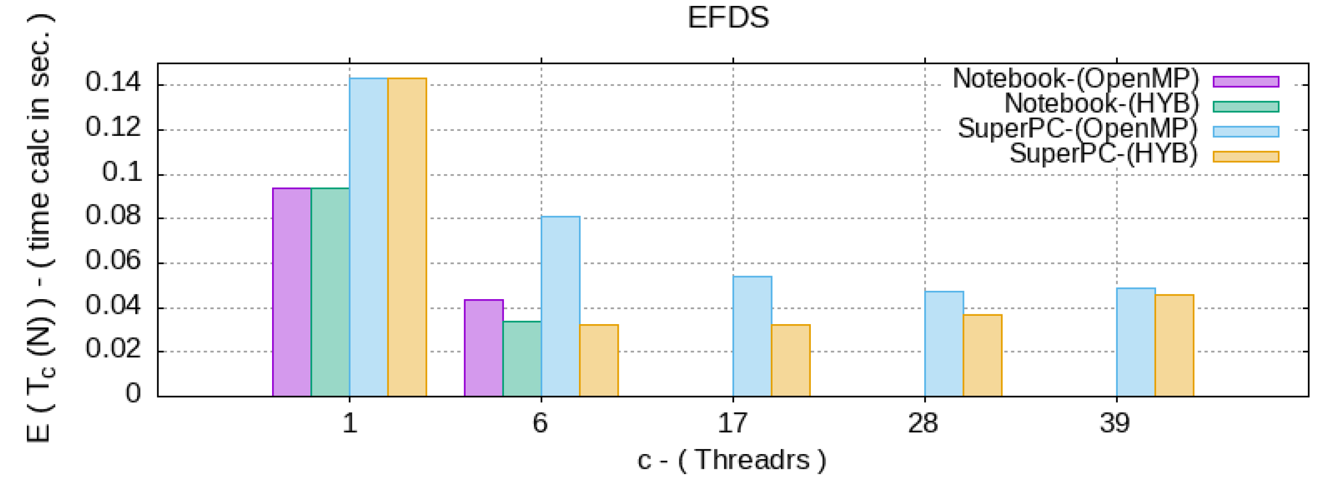
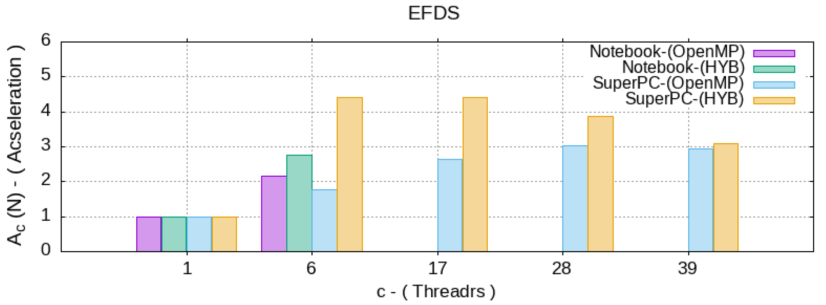
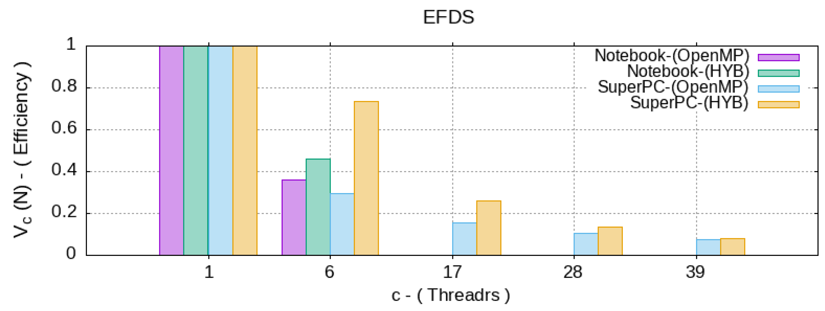
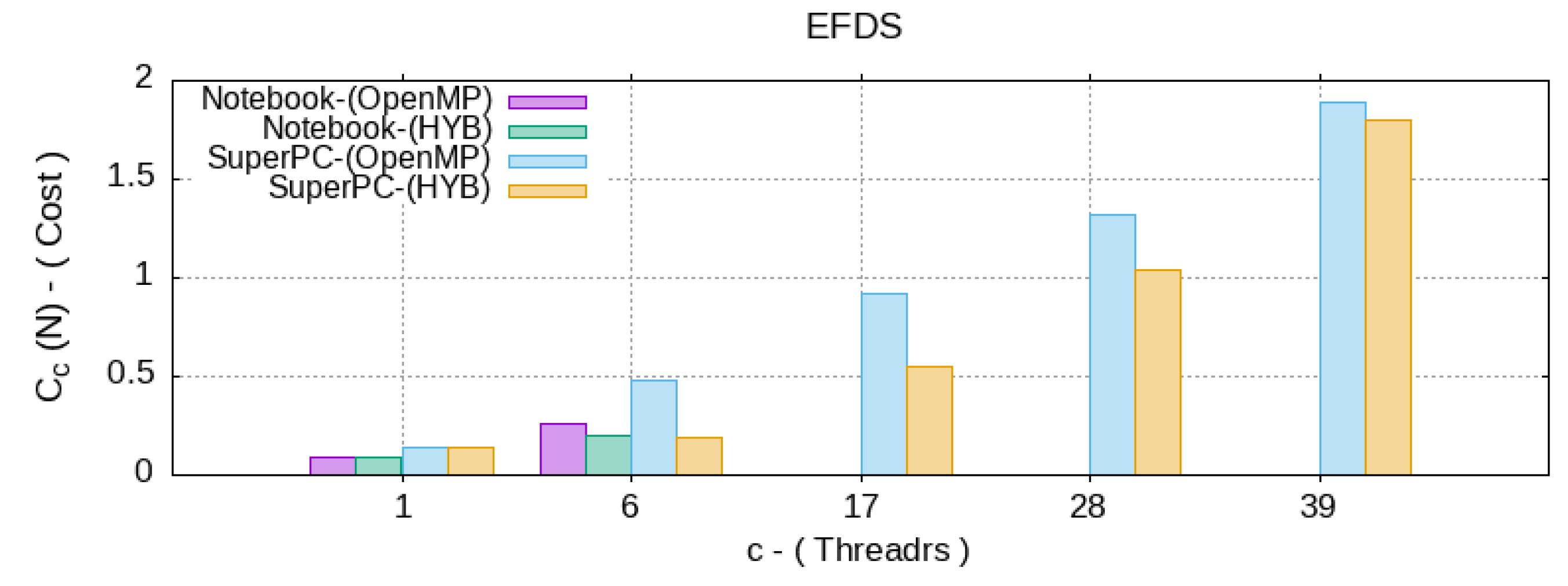
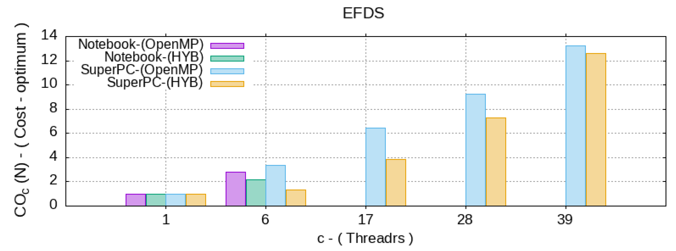
5. Analysis of Computational Efficiency

We investigated how much faster the algorithms with parameter N were characterized by the complexity of the algorithm that implements (3). We compared the computation time of the schemes on the following: one CPU thread (sequential algorithm) and multiple other threads (parallel algorithm). The number of threads and other GPU resources in the developed program were determined and set automatically in an optimal way.

We will conduct experiments on the following computing systems with a different number of threads. The first system will be a laptop, i.e., a HP Pavilion Gaming Laptop Z270X 15-dk0xxx, which was used for the development, debugging, and running of the computational experiments. The laptop had the following specifications: CPU: Intel(R) Core(TM) i5-9300H CPU @ 2.40 GHz (4 CPUs, 8 Threads); RAM: 8192 Mb; GPU: NVIDIA GeForce GTX 1650, GPU @ 16 Multiprocessors 1.56 GHz (1024 CUDA cores), 4102 Mb. The second system is a personal supercomputer NVIDIA DGX STATION with a single multi-threaded CPU, which we also used for computational experiments. This supercomputer has the following specifications: CPU: Intel(R) Xeon(R) CPU E5-2698 v4 @ 2.20 GHz(∼1.20 GHz) (20 CPUs, 40 Threads); RAM: 263,855 Mb; GPU ×4: NVIDIA Tesla V100-DGXS, GPU @ 80 Multiprocessors 1.53 GHz (5120 CUDA cores), 34,084 Mb. The personal supercomputer NVIDIA DGX STATION was located at the Institute of Mathematics that was named after V.I. Romanovsky of the Academy of Sciences of the Republic of Uzbekistan.

It follows from Brent’s lemma [28,44,45] that any algorithm implemented for execution in PRAM-type systems can be modified so that it can be executed in PRAM systems with a smaller number of threads, where PRAM is a random access memory parallel machine combining c threads (cores or CPUs), shared memory, and a control device. This is one of the most common models of computing systems [28]. It means that we can run the developed parallel algorithm on systems that have a different number of cores or threads.

Remark 7. 

We will measure the time spent on code execution—since midnight on 1 January 1970—using the gettimeofday() function, which returns seconds and microseconds to the tv\_sec and tv\_usec fields of the tv\_usec structure, respectively. This is one of the most accurate methods of calculating program execution time. The method is implemented in two functions: tic() —starts measuring, and toc() —stops measuring and then calculates the time spent.

To measure the computation time, consider a model (2) with the following parameters: $\alpha \left(t\right)=0.9-\frac{0.1t}{T}$; $a\left(t\right)=\frac{{cos}^2\left(t\right)}{T}$ ; $b\left(t\right)=1-\frac{0.1t}{T}$; $c\left(t\right)=\frac{{sin}^2\left(t\right)}{T}$ ; $N=2000$; $T=20$. The result of the EFDS calculation (3) is shown in Figure 2:

According to [28] (p. 20), we introduced the following notions:

• $N=2000$—the number of computational grid nodes in the scheme (3), which characterizes the N complexity of the algorithm;
• $T_1\left(N\right)$—the time spent by a sequential algorithm to solve a problem of complexity N;
• $T_c\left(N\right)$—the time taken by the parallel OpenMP algorithm on machine $c>1$ by CPU threads;
• $T_{c,g}\left(N\right)$—the time spent by the hybrid algorithm on a machine $c>1$ by CPU threads, with the presence of parallel code blocks like OpenMP and CUDA. Since the user does not control the number of GPU multiprocessors involved, but specifies only the number of thread per block by choosing the optimal one, then g—does not change.

Since we will obtain a slightly different $T_c$ with each new numerical experiment, and the number of experiments is finite, $T_c$ can be considered a random variable with some distribution function. Then, to compute $T_1\left(N\right)$ and $T_c\left(N\right)$, we resort to the concept of mathematical expectation (average value) [46] for a discrete random variable:

$$\mathbb{E}\left(T_c\left(N\right)\right)=\sum _{i=1}^L\frac{T_c^i\left(N\right)}{L},$$

(5)

where i is the index of the numerical experiment, and L is the sample size.

Then, for the developed algorithm, we determine the $\mathbb{E}\left(·\right)$ mean (5) of a sample of $L=10$ values with the different number of c CPU threads used. The results for the hybrid code are presented in the

Table 1. Time spent T (in seconds) and RAM memory (in Mb) for calculating the sequential algorithm ($T_1$ (N)) and parallel algorithm based on OpenMP (with a different number of threads) implementing EFDS.

	Notebook	Notebook	SuperPC	SuperPC	SuperPC	SuperPC	SuperPC
i	${\mathit{T}}_{\mathbf{1}}\left(\mathit{N}\right)$	${\mathit{T}}_{\mathbf{6}}\left(\mathit{N}\right)$	${\mathit{T}}_{\mathbf{1}}\left(\mathit{N}\right)$	${\mathit{T}}_{\mathbf{6}}\left(\mathit{N}\right)$	${\mathit{T}}_{\mathbf{17}}\left(\mathit{N}\right)$	${\mathit{T}}_{\mathbf{28}}\left(\mathit{N}\right)$	${\mathit{T}}_{\mathbf{39}}\left(\mathit{N}\right)$
1	0.087	0.046	0.145	0.08	0.051	0.047	0.044
2	0.087	0.042	0.144	0.082	0.056	0.047	0.049
3	0.089	0.041	0.147	0.082	0.05	0.054	0.052
4	0.116	0.044	0.125	0.082	0.052	0.049	0.048
5	0.088	0.043	0.146	0.081	0.055	0.047	0.046
6	0.087	0.044	0.157	0.081	0.054	0.049	0.05
7	0.088	0.044	0.144	0.079	0.057	0.05	0.05
8	0.120	0.041	0.125	0.081	0.051	0.05	0.047
9	0.087	0.043	0.149	0.081	0.052	0.04	0.048
10	0.088	0.044	0.147	0.079	0.061	0.04	0.05
$\mathbb{E}\left(T\right)$	0.093	0.043	0.142	0.08	0.053	0.047	0.048
RAM	0.056	8.056	0.056	8.056

below. To compare the results of the analysis, in

Table 2. The time spent T (in seconds) and RAM (in Mb) for calculating the sequential algorithm $T_1$ (N) and hybrid OpenMP–CUDA algorithm (with a different number of threads) implementing EFDS.

	Notebook	Notebook	SuperPC	SuperPC	SuperPC	SuperPC	SuperPC
i	${\mathit{T}}_{\mathbf{1}}\left(\mathit{N}\right)$	${\mathit{T}}_{\mathbf{6},\mathit{g}}\left(\mathit{N}\right)$	${\mathit{T}}_{\mathbf{1}}\left(\mathit{N}\right)$	${\mathit{T}}_{\mathbf{6},\mathit{g}}\left(\mathit{N}\right)$	${\mathit{T}}_{\mathbf{17},\mathit{g}}\left(\mathit{N}\right)$	${\mathit{T}}_{\mathbf{28},\mathit{g}}\left(\mathit{N}\right)$	${\mathit{T}}_{\mathbf{39},\mathit{g}}\left(\mathit{N}\right)$
1	0.087	0.034	0.145	0.031	0.032	0.047	0.037
2	0.087	0.034	0.144	0.031	0.031	0.032	0.049
3	0.089	0.033	0.147	0.031	0.032	0.036	0.05
4	0.116	0.034	0.125	0.038	0.032	0.037	0.05
5	0.088	0.034	0.146	0.031	0.032	0.032	0.039
6	0.087	0.034	0.157	0.031	0.032	0.035	0.049
7	0.088	0.035	0.144	0.038	0.032	0.048	0.051
8	0.120	0.034	0.125	0.031	0.032	0.035	0.048
9	0.087	0.034	0.149	0.031	0.037	0.035	0.05
10	0.088	0.034	0.147	0.031	0.032	0.033	0.039
$\mathbb{E}\left(T\right)$	0.093	0.034	0.1429	0.032	0.032	0.037	0.046
RAM	0.056	16.05	0.056	16.05
RAM (GPU)	-	16.05	-	16.05

, we will provide data on the $\mathbb{E}\left(·\right)$ EFDS (3) calculation time by a parallel algorithm based on OpenMP.

Graphically, the results of computing $\mathbb{E}\left(·\right)$ to the average computation time, from Table 1 and Table 2, by all the specified algorithms are shown in Figure 3 below:

Now, by using the data on the time spent on code execution we can study the efficiency of the parallel algorithm. Efficiency is defined as the optimal ratio in coordinates: where computational speedup is the RAM memory footprint when compared to the sequential version of the algorithm. The average computation time is analyzed in terms of the following: running time, acceleration, efficiency, and the cost of the algorithm.

Definition 2. 

The acceleration $A_c\left(N\right)$ that a parallel algorithm provides on a c—threaded computing system when compared to the most efficient sequential algorithm is defined by the following formula:

$$A_c\left(N\right)={\displaystyle \frac{\mathbb{E}\left(T_1\left(N\right)\right)}{\mathbb{E}\left(T_c\left(N\right)\right)}},$$

(6)

where $\max \left(A_c\left(N\right)\right)=c$ is a theoretical value that is possible in the absence of unavoidable time delays when executing a parallel algorithm, i.e., when there are no additional actions on the interaction between threads, then all calculations are evenly distributed among the threads and no actions are required to merge the results of the calculations.

Definition 3. 

The efficiency $V_c\left(N\right)$ of using a given number of threads by a parallel algorithm is determined by the formula:

$$V_c\left(N\right)={\displaystyle \frac{\mathbb{E}\left(T_1\left(N\right)\right)}{c·\mathbb{E}\left(T_c\left(N\right)\right)}}={\displaystyle \frac{A_c\left(N\right)}{c}},$$

(7)

where, for $max{A}_c\left(N\right)=c$, we get $max\left(E_c\left(N\right)\right)=1$.

Definition 4. 

The cost $C_c\left(N\right)$ is the product of the number of threads used and the $T_c\left(N\right)$ of the solution time by the parallel algorithm:

$$C_c\left(N\right)=\mathbb{E}\left(T_c\left(N\right)\right)·c.$$

(8)

Definition 5. 

The cost-optimal $C{O}_c\left(N\right)$ of an algorithm is characterized by the cost proportional to the complexity of the best sequential algorithm [47]. And in this case, we have the following:

$$C{O}_c\left(N\right)={\displaystyle \frac{C_c\left(N\right)}{\mathbb{E}\left(T_1\left(N\right)\right)}}.$$

(9)

6. Discussion

From the comparison of the analysis results of the proposed algorithms in Figure 4, Figure 5, Figure 6 and Figure 7, we can see that there is a significant acceleration (6) in the computation speed by 3–5 times for parallel algorithms, but when the number of processors/threads for parallel processing increases, their efficiency (7) decreases significantly.

From Figure 4, according to the acceleration data, with the same parameters of the numerical experiment, both computing systems on 6 and 40 maximum available threads were used. This produced the desired result for an approximately equal computation time. At the same time, when running the calculations on a supercomputer on more than 15–20 threads, there was no performance gain.

As a result, the resource/computation time ratio (8) and (9) were inversely proportional to the efficiency, which grew significantly for the parallel algorithms. However, the hybrid OpenMP–CUDA algorithm showed a lower cost than the parallel OpenMP. This means that the presented hybrid algorithm is more efficient both on a supercomputer and on a personal computer.

It can be concluded that it is more than possible to use powerful personal computers and laptops for efficient computations in fractional dynamics models that are based on the Cauchy problem for nonlinear equations of the form (2). In particular, this applies with the fractional derivatives of the Gerasimov–Caputo type (1).

In such a case, the use of supercomputing can be an important future prospect. Non-efficiently loaded threads can be used for the parallel computation of several copies of a numerical algorithm, which will be useful in solving inverse problems for (2). For the solution of inverse problems, an important and well-studied class of mathematical problems found its application in the various fields of science and technology [48]. Their solution is the next stage of the authors of this study’s research, which was conducted to find an application of the described model (2) when based on the fractional derivatives of [34].

Within the framework of this direction, the issues related to the emanation of radon gas [41] through the geo-environment were investigated, particularly when describing the processes of its accumulation and dissipation from the storage chamber with registration sensors. Radon ${}^{222}$Rn was read as a known, informative, and well-established earthquake precursor [49,50]. The solution of the inverse problems were carried out in order to restore some of the parameters of the mathematical model of the dynamic process—one that was based on the known observed data. The solution is extremely time-consuming in itself, and the better efficiency of the hybrid OpenMP–CUDA algorithm will make it possible to solve them in much less time.

7. Conclusions

A software implementation of a non-local explicit finite-difference scheme for solving the fractional Riccati equation as an efficient parallel hybrid OpenMP–CUDA algorithm was presented.

The efficiency of the proposed hybrid OpenMP–CUDA algorithm was analyzed. As a result, for the non-local explicit finite-difference scheme, a significant performance gain of 3–5 times was shown when compared to the best sequential counterpart, as well as a better efficiency when compared to the OpenMP parallel algorithm.

References

1. Nahushev, A.M. Fractional Calculus and Its Application; Fizmatlit: Moscow, Russia, 2003; p. 272. (In Russian) [Google Scholar]
2. Uchaikin, V.V. Fractional Derivatives for Physicists and Engineers. Vol. I. Background and Theory; Springer: Berlin/Heidelberg, Germany, 2013; p. 373. [Google Scholar] [CrossRef] [Green Version]
3. Pskhu, A.V. Fractional Partial Differential Equations; Science: Moscow, Russia, 2005; p. 199. (In Russian) [Google Scholar]
4. Samko, S.G.; Kilbas, A.A.; Marichev, O.I. Fractional Integrals and Derivatives and Some of Their Applications; Science and Tech: Minsk, Belarus, 1987; p. 688. (In Russian) [Google Scholar]
5. Kilbas, A.A.; Srivastava, H.M.; Trujillo, J.J. Theory and Applications of Fractional Differential Equations; Elsevier: Amsterdam, The Netherlands, 2006; p. 523. [Google Scholar]
6. Ortigueira, M.D.; Machado, J.T. What is a fractional derivative? J. Comput. Phys. 2015, 321, 4–13. [Google Scholar] [CrossRef]
7. Ortigueira, M.D.; Valerio, D.; Machado, J.T. Variable order fractional systems. Commun. Nonlinear Sci. Numer. Simul. 2019, 71, 231–243. [Google Scholar] [CrossRef]
8. Patnaik, S.; Hollkamp, J.P.; Semperlotti, F. Applications of variable-order fractional operators: A review. Proc. R. Soc. A 2020, 476, 20190498. [Google Scholar] [CrossRef] [PubMed] [Green Version]
9. Mandelbrot, B.B. The Fractal Geometry of Nature; W.H. Freeman and Co.: New York, NY, USA, 1982; p. 468. [Google Scholar]
10. Volterra, V. Sur les équations intégro-différentielles et leurs applications. Acta Math. 1912, 35, 295–356. [Google Scholar] [CrossRef]
11. Volterra, V. Theory of Functionals and of Integral and Integro-Differential Equations; Dover Publications: New York, NY, USA, 1959; p. 226. [Google Scholar]
12. Petras, I. Fractional-Order Nonlinear Systems: Modeling, Analysis and Simulation; Springer: Berlin/Heidelberg, Germany, 2011; p. 218. [Google Scholar]
13. Sun, H.; Chang, A.; Zhang, Y.; Chen, W. A review on variable-order fractional differential equations: Mathematical foundations, physical models, numerical methods and applications. Fract. Calc. Appl. Anal. 2019, 22, 27–59. [Google Scholar] [CrossRef] [Green Version]
14. Tarasov, V.E. Mathematical Economics: Application of Fractional Calculus. Mathematics 2020, 8, 660. [Google Scholar] [CrossRef]
15. Jeng, S.; Kilicman, A. Fractional Riccati Equation and Its Applications to Rough Heston Model Using Numerical Methods. Symmetry 2020, 12, 959. [Google Scholar] [CrossRef]
16. Rossikhin, Y.A.; Shitikova, M.V. Application of fractional calculus for dynamic problems of solid mechanics: Novel trends and recent results. Appl. Mech. Rev. 2010, 63, 010801. [Google Scholar] [CrossRef]
17. Jamil, B.; Anwar, M.S.; Rasheed, A.; Irfan, M. MHD Maxwell flow modeled by fractional derivatives with chemical reaction and thermal radiation. Chin. J. Phys. 2020, 67, 512–533. [Google Scholar] [CrossRef]
18. Acioli, P.S.; Xavier, F.A.; Moreira, D.M. Mathematical Model Using Fractional Derivatives Applied to the Dispersion of Pollutants in the Planetary Boundary Layer. Bound.-Layer Meteorol. 2019, 170, 285–304. [Google Scholar] [CrossRef]
19. Fellah, M.; Fellah, Z.E.A.; Mitri, F.; Ogam, E.; Depollier, C. Transient ultrasound propagation in porous media using Biot theory and fractional calculus: Application to human cancellous bone. J. Acoust. Soc. Am. 2013, 133, 1867–1881. [Google Scholar] [CrossRef]
20. Mainardi, F. Fractional Calculus and Waves in Linear Viscoelastisity: An Introduction to Mathematical Models, 2nd ed.; World Scientific Publishing Company: Singapore, 2022; p. 625. [Google Scholar]
21. Cai, M.; Li, C. Theory and Numerical Approximations of Fractional Integrals and Derivatives; Society for Industrial and Applied Mathematics: Philadelphia, PA, USA, 2020; p. 317. [Google Scholar] [CrossRef] [Green Version]
22. Bogaenko, V.A.; Bulavatskiy, V.M.; Kryvonos, I.G. On Mathematical modeling of Fractional-Differential Dynamics of Flushing Process for Saline Soils with Parallel Algorithms Usage. J. Autom. Inf. Sci. 2016, 48, 1–12. [Google Scholar] [CrossRef]
23. Bogaenko, V.O. Parallel finite-difference algorithms for three-dimensional space-fractional diffusion equation with phi–Caputo derivatives. Comput. Appl. Math. 2020, 39, 163. [Google Scholar] [CrossRef]
24. Gerasimov, A.N. Generalization of linear deformation laws and their application to internal friction problems. Appl. Math. Mech. 1948, 12, 529–539. [Google Scholar]
25. Caputo, M. Linear models of dissipation whose Q is almost frequency independent—II. Geophys. J. Int. 1946, 13, 529–539. [Google Scholar] [CrossRef]
26. Daintith, J.; Wright, E. A Dictionary of Computing; Oxford University Press: Oxford, UK; p. 583.
27. Miller, R.; Boxer, L. Algorithms Sequential and Parallel: A Unified Approach, 3rd ed.; Cengage Learning: Boston, MA, USA, 2013; p. 417. [Google Scholar]
28. Borzunov, S.V.; Kurgalin, S.D.; Flegel, A.V. Workshop on Parallel Programming: A Study Guide; BVH: Saint Petersburg, Russia, 2017; p. 236. (In Russian) [Google Scholar]
29. Kalitkin, N.N. Numerical Methods, 2nd ed.; BVH: Saint Petersburg, Russia, 2011; p. 592. (In Russian) [Google Scholar]
30. Sanders, J.; Kandrot, E. CUDA by Example: An Introduction to General-Purpose GPU Programming; Addison-Wesley Professional: London, UK, 2010; p. 311. [Google Scholar]
31. Okrepilov, V.V.; Makarov, V.L.; Bakhtizin, A.R.; Kuzmina, S.N. Application of Supercomputer Technologies for Simulation of Socio-Economic Systems. R-Economy 2015, 1, 340–350. [Google Scholar] [CrossRef] [Green Version]
32. Il’in, V.P.; Skopin, I.N. About performance and intellectuality of supercomputer modeling. Program. Comput. Softw. 2016, 42, 5–16. [Google Scholar] [CrossRef]
33. Machado, J.T.; Kiryakova, V.; Mainardi, F. Recent history of fractional calculus. Commun. Nonlinear Sci. Numer. Simul. 2011, 16, 1140–1153. [Google Scholar] [CrossRef] [Green Version]
34. Tverdyi, D.A.; Parovik, R.I. Investigation of Finite-Difference Schemes for the Numerical Solution of a Fractional Nonlinear Equation. Fractal Fract. 2022, 6, 23. [Google Scholar] [CrossRef]
35. Tvyordyj, D.A. Hereditary Riccati equation with fractional derivative of variable order. J. Math. Sci. 2021, 253, 564–572. [Google Scholar] [CrossRef]
36. Tverdyi, D.A.; Parovik, R.I. Application of the Fractional Riccati Equation for Mathematical Modeling of Dynamic Processes with Saturation and Memory Effect. Fractal Fract. 2022, 6, 163. [Google Scholar] [CrossRef]
37. Tverdyi, D.A.; Parovik, R.I. Fractional differential model of physical processes with saturation and its application to the description of the dynamics of COVID-19. Bull. KRASEC Phys. Math. Sci. 2022, 40, 119–137. [Google Scholar] [CrossRef]
38. Tverdyi, D.A.; Parovik, R.I. Mathematical modeling in MATLAB of solar activity cycles according to the growth-decline of the Wolf number. Bull. KRASEC Phys. Math. Sci. 2022, 41, 47–64. [Google Scholar] [CrossRef]
39. Taogetusang, S.; Li, S. New application to Riccati equation. Chin. Phys. B 2010, 19, 080303. [Google Scholar] [CrossRef]
40. Parovik, R.I. Mathematical models of oscillators with memory. In Oscillators—Recent Developments; IntechOpen: London, UK, 2019; pp. 3–21. [Google Scholar] [CrossRef] [Green Version]
41. Tverdyi, D.A.; Makarov, E.O.; Parovik, R.I. Hereditary Mathematical Model of the Dynamics of Radon Accumulation in the Accumulation Chamber. Mathematics 2023, 11, 850. [Google Scholar] [CrossRef]
42. Sun, H.; Chen, W.; Li, C.; Chen, Y. Finite difference schemes for variable-order time fractional diffusion equation. Int. J. Bifurc. Chaos 2012, 22, 1250085. [Google Scholar] [CrossRef] [Green Version]
43. Parovik, R.I. On a finite-difference scheme for an hereditary oscillatory equation. J. Math. Sci. 2021, 253, 547–557. [Google Scholar] [CrossRef]
44. Brent, R.P. The parallel evaluation of general arithmetic expressions. J. Assoc. Comput. Mach. 1974, 21, 201–206. [Google Scholar] [CrossRef] [Green Version]
45. Corman, T.H.; Leiserson, C.E.; Rivet, R.L.; Stein, C. Introduction to Algorithms, 3rd ed.; The MIT Press: Cambridge, UK, 2009; p. 1292. [Google Scholar]
46. Shao, J. Mathematical Statistics, 2nd ed.; Springer: New York, NY, USA, 2003; p. 592. [Google Scholar]
47. Gergel, V.P.; Strongin, R.G. High Performance Computing for Multi-Core Multiprocessor Systems. Study Guide; Moscow State University Publishing: Moscow, Russia, 2010; p. 544. (In Russian) [Google Scholar]
48. Mueller, J.L.; Siltanen, S. Linear and Nonlinear Inverse Problems with Practical Applications; Society for Industrial and Applied Mathematics: Philadelphia, PA, USA, 2012; p. 351. [Google Scholar] [CrossRef]
49. Cicerone, R.D.; Ebel, J.E.; Beitton, J. A systematic compilation of earthquake precursors. Tectonophysics 2009, 476, 371–396. [Google Scholar] [CrossRef]
50. Firstov, P.P.; Makarov, E.O.; Gluhova, I.P.; Budilov, D.I.; Isakevich, D.V. Search for predictive anomalies of strong earthquakes according to monitoring of subsoil gases at Petropavlovsk-Kamchatsky geodynamic test site. Geosyst. Transit. Zones 2018, 2, 16–32. (In Russian) [Google Scholar] [CrossRef]
Figure 1. Simplified CPU and GPU hardware circuits (from materials http://www.nvidia.ru, accessed on 10 May 2023).
Mathematics 11 03358 g001
Figure 2. EFDS calculation result (3).
Mathematics 11 03358 g002
Figure 3. Average E · calculation time, in seconds, for different c—i.e., the number of CPU threads.
Mathematics 11 03358 g003
Figure 4. Acceleration A c ( N ) for the different c—number of CPU threads.
Mathematics 11 03358 g004
Figure 5. Efficiency of V c ( N ) for the different c—number of CPU threads.
Mathematics 11 03358 g005
Figure 6. Cost of the C c ( N ) algorithm for the different c—number of CPU threads.
Mathematics 11 03358 g006
Figure 7. Cost-optimal indicator C O c ( N ) for the different c—number of CPU threads.
Mathematics 11 03358 g007