On a Fast Hough/Radon Transform as a Compact Summation Scheme over Digital Straight Line Segments

Abstract

The Hough transform, interpreted as the discretization of the Radon transform, is a widely used tool in image processing and machine vision. The primary way to speed it up is to employ the Brady–Yong algorithm. However, the accuracy of the straight line discretization utilized in this algorithm is limited. In this study, we propose a novel algorithm called $ASD2$ that offers fast computation of the Hough transform for images of arbitrary sizes. Our approach adopts a computation scheme similar to the Brady–Yong algorithm but incorporates the best possible line discretization for improved accuracy. By employing the Method of Four Russians, we demonstrate that for an image of size $n\times n$ where $n=8^q$ and $q\in \mathbb{N}$, the computational complexity of the $ASD2$ algorithm is $O\left(n^{8/3}\right)$ when summing over $O\left(n^2\right)$ digital straight line segments.

1. Introduction

In this paper, we propose a new fast algorithm for calculating sums along a large number of discrete lines in an image. Such algorithms are called fast Hough transform (fast HT, FHT) or fast discrete Radon transform algorithms [1]. HT was initially positioned as a method for identifying certain graphic primitives in images, such as lines, ellipses, or their segments [2]. Over time, its scope of application has significantly expanded. Some examples of HT application areas that are very far from the search for segments include color segmentation and determination of illumination chromaticity [3,4,5], as well as automatic determination of optical aberration parameters [6,7,8].

Similarly to Fourier transform, HT requires fast algorithms for its calculation. The use of fast algorithms is all the more justified the higher the requirements for computational efficiency in the applied problem being solved. Especially stringent performance requirements are imposed on the visual systems of unmanned vehicles. The hardware of such systems can be configured according to the requirements for weight, dimensions, and power consumption, so the computational optimization of the algorithms used on a particular computer becomes extremely important. Therefore, fast algorithms for HT computation have become an almost integral part of such systems. They are most often used to search for road marking elements [9,10], and many authors have created algorithms designed for embedded devices [11,12,13].

The problem of energy efficiency is also key for systems running on mobile devices [14], which also actively use fast HT calculation. Document recognition systems use HT to search for quadrangles of document boundaries [15,16,17] or for parallel-segment patterns. Parallel beam search algorithms using FHT can find the slope of a document [18,19,20] or its individual characters [21,22] in an image. Another part of the recognition process on mobile devices that uses FHT is barcode detection [23].

For somewhat different reasons, FHT is used in X-ray computed tomography [1,24,25,26]. With significant computing resources involved, the desired reconstruction resolution parameters have not yet been achieved, so the volumes of processed data are constantly growing, which, when using asymptotically inefficient algorithms, sooner or later leads to a resource shortage. On the contrary, using the correct algorithmic base allows for a much more flexible approach to managing the applied resources. In addition, the task of speeding up reconstruction is extremely relevant for a new class of online methods that allow for real-time evaluation and correction of tomographic measurement parameters [27].

What is interesting is that the use of classical algorithms with FHT does not contradict the development of neural network methods but allows them to be more computationally efficient. A new field in recognition is the construction of so-called Hough networks based on classical convolutional networks. Such networks include an untrainable layer that calculates the discretization of the Radon transform. This layer allows for the extraction of information about lines and segments in an image, even if the receptive fields of convolutional neurons are small, unlike classical convolutional layers [28,29,30]. This effect is most easily demonstrated by comparing neural network line and segment search methods [31,32]. In recognizing more complex objects with deep learning methods, using FHT also improves the ratio of recognition accuracy and the required amount of computations [33,34]. In addition, currently the main architectures used in neural network tomographic reconstruction methods contain Hough/Radon layers [35,36,37].

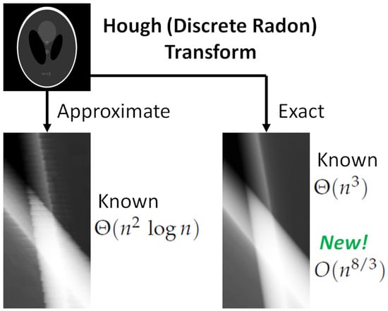
This paper proposes a new Hough transform fast computation algorithm that is more accurate than the Brady–Yong algorithm [1].

2. Related Works

The Hough transform in image processing is usually understood as a method of robust estimation of the parameters of one or more lines in a discrete image by counting the number of points lying on each set of discrete lines. The method is named after Paul V. C. Hough, who first proposed it in 1959 [38] and, in 1962, received, on its basis, the patent, “Method and means for recognizing complex patterns” [39]. It is noteworthy that neither the original publication nor Hough’s patent provides a formal definition of the proposed transform. Neither text contains a single mathematical formula. In his historical excursus on the invention of HT, authoritative researcher in classical visual pattern recognition Peter Hart claims [40] that it was Azriel Rosenfeld who first formalized HT, at least partially, in his book on image processing that was published in 1969 [41]. HT (and its very name) gained wide popularity following the publication in of an article in 1972 coauthored by Richard Duda and Peter Hart himself [2].

In 1981, Stanley Deans drew attention [42] to the extreme similarity of the Hough transform and the Radon transform introduced by the latter back in 1917 [43]. In his work, Deans argues that the Radon transform has all the properties of HT (according to R. Duda and P. Hart’s interpretation [2]) and proposes the generalization of the Radon transform for curved lines. In their detailed review devoted to HT published in 1988 [44], J. Illingworth and J. Kittler consider, among other things, the work of S. Deans and claim that HT is a special case of the Radon transform, adding that when it comes to binary images, the transforms coincide.

In 1992, Martin Brady and Whanki Yong published a paper on the fast approximate discrete Radon transform [1] for square images of linear size $n\stackrel{\mathrm{def}}{=}{2}^q$, $q\in \mathbb{N}$. In its annotation and conclusion, the authors use the names of the Hough and Radon transforms interchangeably. The method they proposed is based on dynamic programming, which is used to skip the repeated calculation of the sums of already processed segments when computing the sum along the line they constitute. This allows for calculation of the HT for an $n\times n$-sized image in $\Theta (n^{2}logn)$ summations (with the complexity of the naive method $\Theta \left(n^3\right)$). Six years later, M. Brady once again published a description of this method, this time without coauthors [45]. 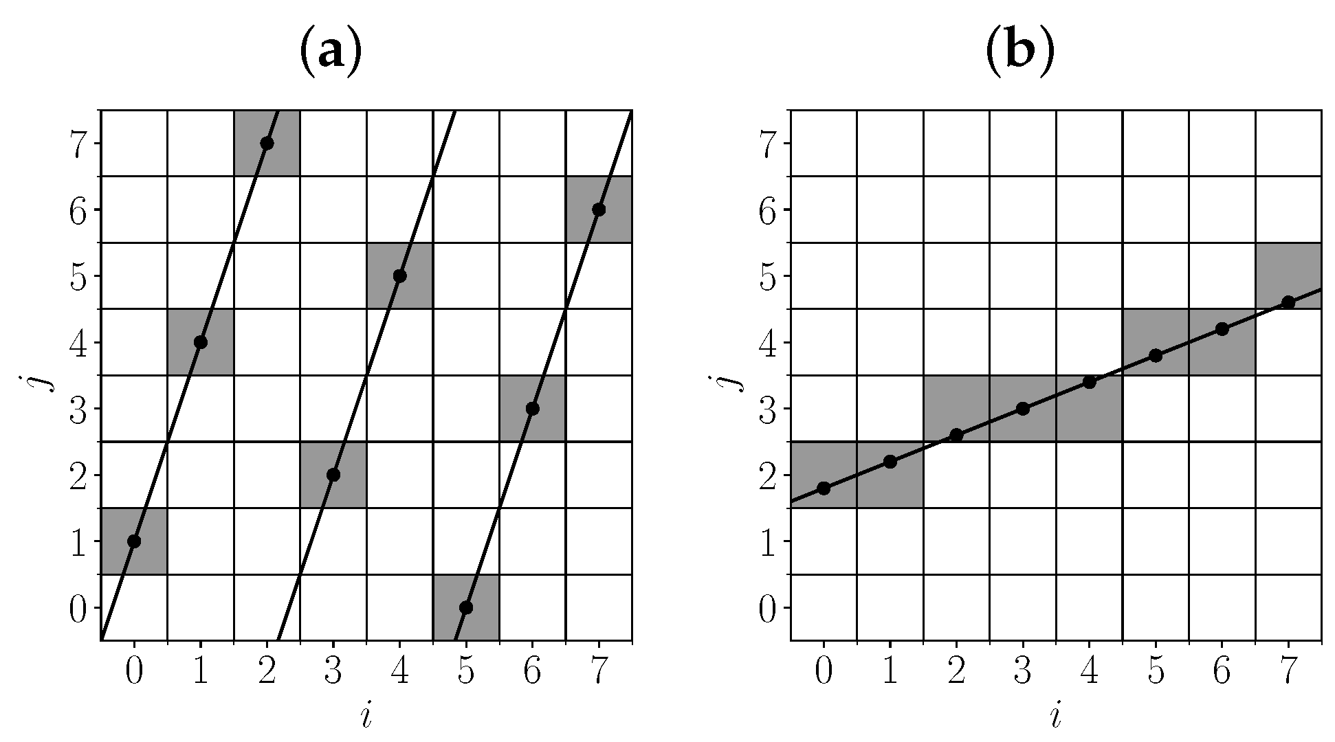Figure 1 explains due to which intersections of patterns (sets of pixel positions) in the discrete case some of the sub-sums participate in the computation of several sums, making it more efficient.

The Brady–Yong method was apparently also independently developed by Walter Götz, who published it in his PhD thesis in German in 1993. This work was reprinted in an English-language article by W. Götz and H. Druckmüller, published twice (in 1995 and 1996) in the same journal [46,47]. The two versions of the article are not completely identical, but their differences are, at first glance, quite minor. Another author who published the same method in 1994 is well-known French algorithmist Jean Vuillemin  [48]. However, all the works mentioned here were published later than those of M. Brady and W. Yong. Therefore, in this paper, the method is referred to by the names of the latter.

The Brady–Yong method is an approximate method in the sense that the pixel sets it sums over are not the best possible line approximations. In 2021, Simon Karpenko and Egor Ershov published a proof that the maximum orthotropic error of approximating geometric lines in the Brady–Yong method is $\left({log}_{2}n\right)/6$ for cases of even binary powers (q) of linear image size $n=2^q$ and $\left({log}_{2}n\right)/6-1/18$ for odd binary powers [49]. Here, the orthotropic error is understood as the error along the y axis for lines defined by the equation $y=kx+b$, $\left|k\right|\le 1$ and along the x axis for lines defined by the equation $x=ky+b$, $\left|k\right|<1$.

Brady’s approach is not the sole method for constructing fast Radon transform algorithms with a computational complexity of $\Omega (n^{2}logn)$. Another approach is the pseudopolar Fourier transform [50]. The algorithm based on this approach is also known as the slant–stack algorithm. Despite having the same asymptotic complexity as the Brady–Yong algorithm, the slant–stack algorithm involves complex multiplications, whereas the Brady–Yong algorithm utilizes only additions and can be easily implemented using integers, thereby allowing for enhanced performance with various SIMD architectures [51]. However, it is important to note that the slant–stack algorithm is not considered to be highly accurate. Levi and Efros [52] showed weight maps defined on the input raster which corresponded to the algorithm’s outputs. These weight maps deviated significantly from the expected line discretization. Furthermore, some weights can be negative, resulting in unexpected effects, where the computed Radon image may contain negative values despite having a non-negative preimage. Consequently, ref. [52] proposed an alternative algorithm that is more accurate but slower in terms of execution. Comparing summation-based algorithms directly with algorithms that use soft line discretization poses challenges because the ideal discrete representation of a line depends on the nature of the input data and the specific problem being addressed. In this study, we focus solely on algorithms that define lines in a binary manner. These representations provide a basis for discussing accuracy.

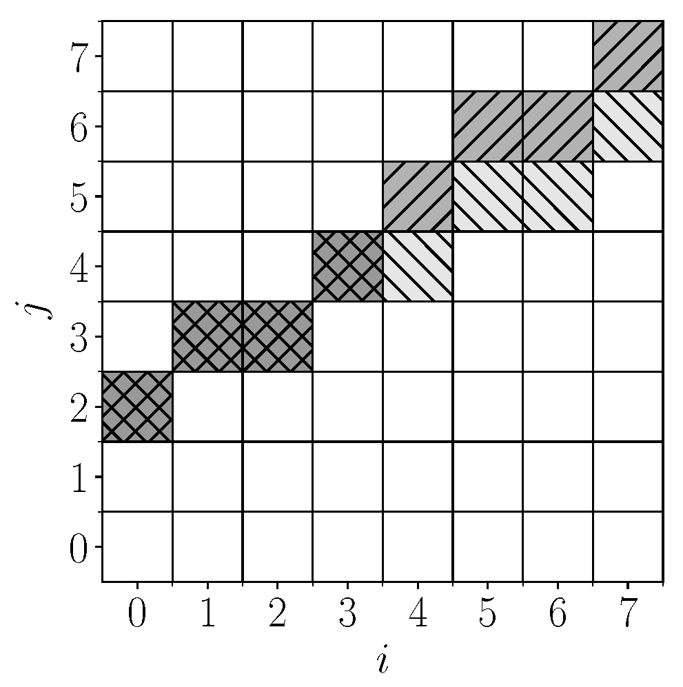
Back in 1974, A. Rosenfeld considered the optimal discretization of line segments, calling its result digital straight line segments (DSLS) [53]. The orthotropic error for DSLS is limited to the constant $1/2$. Thus, even for images with size $n=16$, the error for discrete Brady–Yong patterns becomes significant compared to DSLS. Figure 2 shows the difference between DSLS and Brady–Yong approximation for a line defined by the equation $j=6i/15$. Figure 3 presents a visualization of the distribution of coordinate error in the Brady–Yong approximation along a line segment for a large image size of $n=4096$.

Regrettably, there is a lack of research studies that assess the extent to which the mentioned geometric deviations influence the accuracy of applied algorithms utilizing the Brady–Yong method. Nevertheless, this does not imply that the impact is insignificant. Namely, in [25] the authors showed that the acceleration of the tomographic reconstruction method through the convolution and backprojection using the Brady–Yong algorithm results in an approximate doubling of the RMSE of the reconstruction, which is a significant quality loss.

According to these facts, two related questions arise: is it possible to build a faster and/or more accurate FHT algorithm than the algorithm proposed by Brady and Yong? The first question, apparently (the work was not peer-reviewed), was answered by Timur Khanipov in 2018 [54], who showed that the complexity of the problem of computing a dense Hough image using Brady–Yong dyadic patterns is $\Omega (n^{2}logn)$, that is, their method cannot be improved in terms of speed. In the same work, T. Khanipov showed that this estimate is also true for DSLS-based FHT computations. The same year, he proposed, apparently for the first time, a method for accelerated DSLS-based FHT computation [55] with an asymptotic computational complexity of $O(n^3/logn)$. Just like the Brady–Yong method, the Khanipov method relies solely on summations and achieves acceleration by reusing common sub-sums. The hierarchy of sub-sums is built through an iterative process of refining patterns, where patterns with different slopes are intersected. In essence, while the Brady–Yong method employs a hierarchical division of the image, the Khanipov method employs a hierarchical division of the pattern set based on the patterns’ slopes. It is important to note that this method is presented as an abstract mathematical scheme, which means that additional efforts are necessary to turn it into a specific algorithm. It is clear that the difference between the achieved complexity and the previously obtained estimate is significant and leaves room for more efficient algorithms and/or more accurate lower bounds.

What is interesting to note here is that the algorithm, which is a fast ($\Theta (n^{2}logn)$) and exact discrete Radon transform, has already been constructed [56]. However, this does not negate the problem under discussion. The fact is that this and other works investigating fast algorithms for computation of the discrete Fourier transform have used a different definition of the discrete Radon transform (going back to the 1988 work of I. Gertner [57]). In it, the sets of raster nodes over which the summation is performed are given by linear congruent sequences. For ${\mathbb{Z}}_n$ residue rings, such sequences are directly analogous to linear functions, but the resulting sets differ significantly from DSLS. In particular, most of them are not connected because for them, k is an integer. Figure 4 illustrates these differences.

Another approach to the development of computational schemes for FHT is to construct fast generalized Hough transforms (FGHTs) [58]. In this method, the development of the FGHT algorithm (including the FHT for DSLS) is treated as an optimization problem and solved numerically. The disadvantages of this approach include the fact that the scheme has to be calculated separately for each size of input image. In addition, the problem of finding the optimal FGHT generally coincides with the NP-complete problem named “ensemble computation” up to notation (p. 66 [59]). At the same time, approximate approaches with acceptable complexity used for this task are rather primitive (they are based on the greedy strategy [58,60]), and their theoretical efficiency is unknown. As a consequence, estimates of the asymptotic complexity of the resulting FHT computational schemes still have not been obtained.

Thus, in this paper, we solve the problem of constructing a fast algorithm for calculation of the Hough/Radon transform, similar to the Brady–Yong algorithm [1]. Unlike the latter, the proposed algorithm uses a more accurate straight line approximation—DSLS. The closest analog is the Khanipov method [55], but our algorithm has a lower asymptotic complexity.

The remainder of this article is structured as follows. Section 3 introduces the necessary definitions, estimates the cardinality of the set of all DSLS in an image, and considers two algorithms for summing over it: naive $AFNA$, which does not reuse matching sub-sums, and accelerated $AFD2$, which uses a divide-and-conquer scheme. Section 4 specifies the DSLS subset of cardinality ($\Theta \left(n^2\right)$) to be calculated and proposes the $AS4R$ algorithm for its computation with $O\left(n^{8/3}\right)$ summations. Section 5 considers the final $ASD2$ algorithm. We show that the number of summations for it is not worse than for $AS4R$. Finally, the complexity of other operations used in the algorithm is estimated, and the conclusion is drawn that they do not worsen the asymptotic estimate. Section 6 recaps and discusses the obtained results.

3. Hough (Discrete Radon) Transform Algorithms for a Full Set of Digital Straight Line Segments

3.1. Basic Definitions and Statements

In this section, we estimate the total number of DSLS approximating straight line segments intersecting an image section of size $w\times h$, $w,h\in \mathbb{N}$ in such a way that both ends of the segment are located on the section boundary. The image section is understood as the rectangle ${\Omega }_{w,h}\stackrel{\mathrm{def}}{=}[-0.5,w-0.5)\times [-0.5,h-0.5)\subset {\mathbb{R}}^2$. The proper image is the mapping $I_{w,h}:{\mathbb{Z}}_{w,h}^2\to \mathbb{A}$, where ${\mathbb{Z}}_{w,h}^2\stackrel{\mathrm{def}}{=}{\mathbb{Z}}_w\times {\mathbb{Z}}_h$ and $(\mathbb{A},+)$ is an Abelian semigroup with a neutral element. $dom{I}_{w,h}$ is called a raster. Raster elements are called positions, and sets (including ordered sets) of the positions are called patterns.

The considered DSLS are expressed in one of two ways depending on the slope of the line being approximated:

$$\begin{array}{cc}\hfill & p_{w,h}^H(k,b)\stackrel{\mathrm{def}}{=}\left\{(i,j)\in {\mathbb{Z}}_{w,h}^2|j=[ki+b]\right\},k\in (-1,1]\subset \mathbb{R},b\in \mathbb{R},\hfill \\ \hfill & p_{w,h}^V(k,b)\stackrel{\mathrm{def}}{=}\left\{(i,j)\in {\mathbb{Z}}_{w,h}^2|i=[kj+b]\right\},k\in [-1,1)\subset \mathbb{R},b\in \mathbb{R}.\hfill \end{array}$$

(1)

The set ($S_{w,h}$) of all considered DSLS is the union of all such patterns and is defined as follows:

$$\begin{array}{cc}\hfill & S_{w,h}\stackrel{\mathrm{def}}{=}{S}_{w,h}^H\cup S_{w,h}^V,\hfill \\ \hfill & S_{w,h}^H\stackrel{\mathrm{def}}{=}\left\{p|\exists k,b:p=p_{w,h}^H(k,b)\wedge p\ne \varnothing \right\},\hfill \\ \hfill & S_{w,h}^V\stackrel{\mathrm{def}}{=}\left\{p|\exists k,b:p=p_{w,h}^V(k,b)\wedge p\ne \varnothing \right\}.\hfill \end{array}$$

(2)

Patterns $p_{w,h}^H(k,b)$ and $p_{h,w}^V(k,b)$ differ only in the order of coordinates; therefore, we do not consider patterns from $S^V$ further. Additionally,

$$\left|S_{w,h}\right|\le \left|S_{w,h}^H\right|+\left|S_{h,w}^H\right|.$$

(3)

Patterns $p_{w,h}^H(k,b)$ and $p_{w,h}^H(-k,-b)$ are symmetric with respect to the first axis; therefore,

$$\left|S_{w,h}\right|\le 2\left|S_{w,h}^{H+}\right|+2\left|S_{h,w}^{H+}\right|,S_{w,h}^{H+}\stackrel{\mathrm{def}}{=}\left\{p|\exists k\ge 0,b:p=p_{w,h}^H(k,b)\wedge p\ne \varnothing \right\},$$

(4)

and the set $S^{H-}\stackrel{\mathrm{def}}{=}{S}^H\setminus S^{H+}$ is also not considered.

In what follows, some conclusions are based on the analysis of sets of S patterns closed with respect to the vertical shift:

$$p\in S\Rightarrow p+(0,1)\in S,p+(\Delta i,\Delta j)\stackrel{\mathrm{def}}{=}\{(i+\Delta i,j+\Delta j)|(i,j)\in p\},$$

(5)

but $S^{H+}$ does not have this property.

Let us define patterns for an image that is cyclically closed along the second coordinate:

$$p_{w,h}^{CH+}(k,b)\stackrel{\mathrm{def}}{=}\left\{(i,j)\in {\mathbb{Z}}_{w,h}^2|j=[ki+b]modh\right\},k\in [0,1]\subset \mathbb{R},b\in \mathbb{R}.$$

(6)

The patterns $p_{w,h+w}^{CH+}(k,b)$ and $p_{w,h}^{H+}(k,b)$ coincide on the raster ${\mathbb{Z}}_{w,h}^2$. Therefore,

$$\left|S_{w,h}\right|\le 2\left|S_{w,w+h}^{CH+}\right|+2\left|S_{h,w+h}^{CH+}\right|,S_{w,h}^{CH+}\stackrel{\mathrm{def}}{=}\left\{p|\exists k,b:p=p_{w,h}^{CH+}(k,b)\wedge p\ne \varnothing \right\}.$$

(7)

All patterns from $S_{w,h}^{CH+}$ include exactly one position in each column of the raster ${\mathbb{Z}}_{w,h}^2$, where the set $S_{w,h}^{CH+}$ has property (5) (with a shift: $\Delta j\in {\mathbb{Z}}_h$), which allows us to introduce the set of generator patterns ($G_{w,h}^{CH+}$):

$$S_{w,h}^{CH+}=\left\{p+(0,\Delta j)|p\in G_{w,h}^{CH+}\cap \Delta j\in {\mathbb{Z}}_h\right\},G_{w,h}^{CH+}\stackrel{\mathrm{def}}{=}\left\{p|p\in S_{w,h}^{CH+}\cap (0,0)\in p\right\}.$$

(8)

where

$$\left|S_{w,h}^{CH+}\right|=h\left|G_{w,h}^{CH+}\right|,\left|S_{w,h}\right|\le 2(w+h)\left(\left|G_{w,w+h}^{CH+}\right|+\left|G_{h,w+h}^{CH+}\right|\right).$$

(9)

In what follows, we solve the problem of constructing sums of image elements ($I_{w,h}$) given by patterns from $S_{w,h}^{CH+}$. This also solves the problem for $S_{w,h}$, since we have traced not only the relationship between the cardinalities of these sets but also the coincidence of the geometry of their elements up to symmetries.

3.2. Digital Straight Line Segment Count

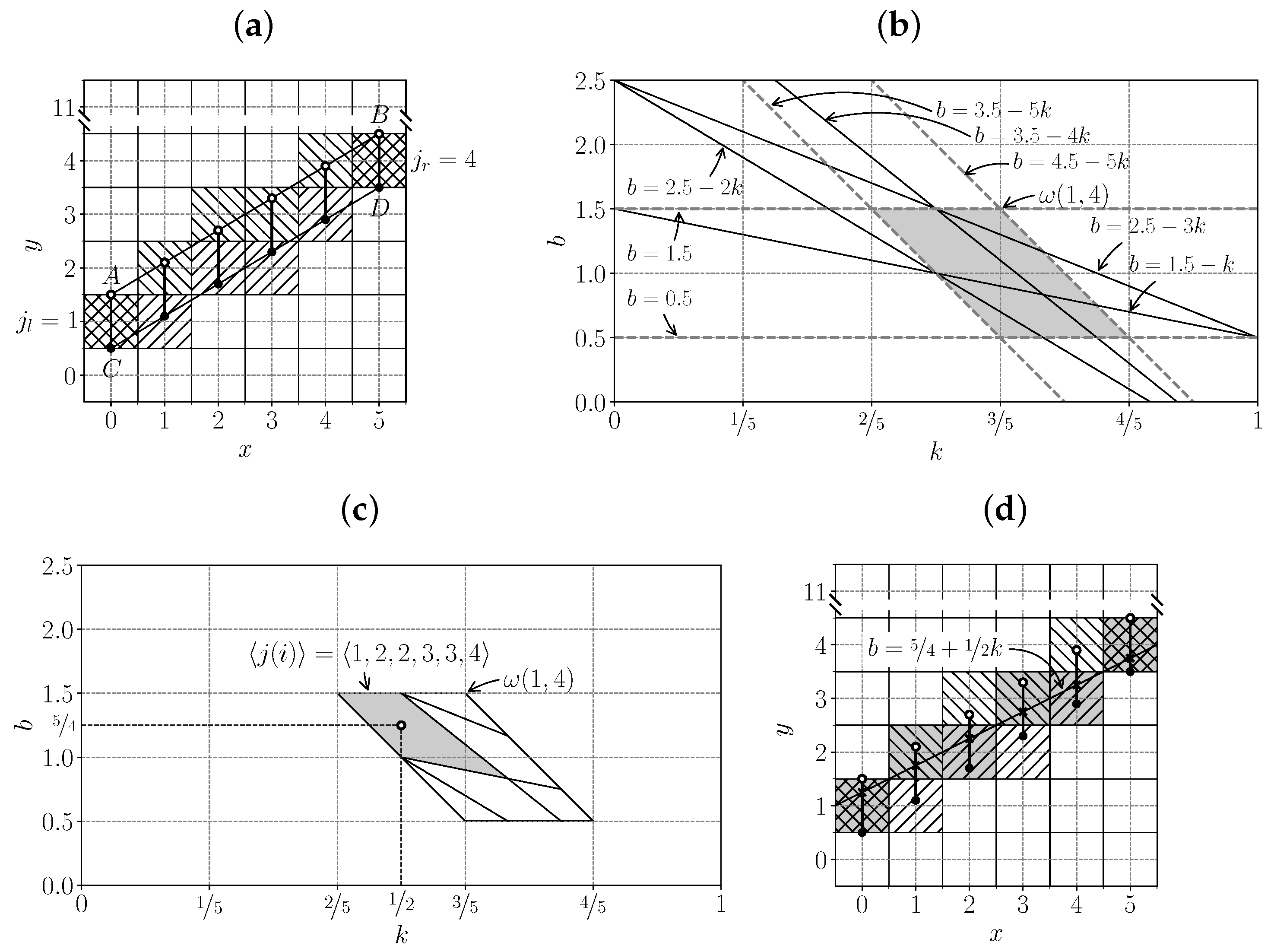
Let us find an upper estimate for $\left|S_{w,h}^{H+}\right|$. To do this, we prove

Theorem 1.

$\left|G_{w,w+h}^{CH+}\right|\le w{n}_1\left(w\right)\le w^3$, where

$$n_1\left(w\right)\stackrel{\mathrm{def}}{=}\frac{(w-2)(w-1)}{2}+1.$$

(10)

Proof. 

Let us estimate the number of patterns from $S_{w,h}^{H+}$ to which the positions $(0,j_l)$ and $(w-1,j_r)$ belong. All such patterns are given by parameter vectors ($(k,b)$) lying in the following parallelogram: $b\in [j_l-0.5,j_l+0.5)$, $k\in \left[{\displaystyle \frac{j_r-b-0.5}{w-1}},{\displaystyle \frac{j_r-b+0.5}{w-1}}\right)$. We denote it as $\omega (j_l,j_r)$. Each of the image columns (i) has no more than two positions that can belong to patterns from the considered set, since

$$\left\{\begin{array}{c}y=kx+b,\hfill \\ (k,b)\in \omega (j_l,j_r)\hfill \end{array}\right.\Rightarrow y\in \left[\frac{j_r-j_l}{w-1}x+j_l-0.5,\frac{j_r-j_l}{w-1}x+j_l+0.5\right),$$

(11)

that is, for $(k,b)\in \omega (j_l,j_r)$ and given i, the rounded value in definition (1) lies in a half interval of length 1, and exactly one half-integer value belongs to such a half interval (see Figure 5a).

We denote the half integer belonging to the half interval (11) for column i as $t_i$. The condition under which $j>t_i$ is satisfied in the position $(i,j)$ specified by definition (1) is linear with respect to the parameters of the following line: $ki+b>t_i$; that is, the choice of one of the two possible positions in column i is determined by the belonging of the point $(k,b)$ from $\omega (j_l,j_r)$ to one of the half planes.

With an image width of w, the choice of one of the two possible pixels occurs in $w-2$ or fewer columns, and the pattern is formed by a combination of solutions in these columns. The boundaries of $ki+b>t_i$ on the plane of parameters $(k,b)$ of the lines form a partition of the region ($\omega (j_l,j_r)$). The original lines with parameters from $\omega (j_l,j_r)$ correspond to the same pattern from $S_{w,h}^{H+}$ if and only if the corresponding points lie in the same partition region (see Figure 5b–d).

The maximum number of regions that can result from dividing a plane by n straight lines is $n(n+1)/2+1$, as shown by Jacob Steiner in 1826 [61]. The same is true for a convex region.

Therefore, the function $n_1\left(w\right)$ bounds from above the number of patterns with parameters from $\omega (j_l,j_r)$. This is particularly true for $\omega (0,j_r)$, where $\left|G_{w,w+h}^{CH+}\right|\le w{n}_1\left(w\right)\le w^3$.    □

Corollary 1.

$\left|S_{w,w+h}^{CH+}\right|\le w{n}_1\left(w\right)(w+h)$.

Corollary 2.

$\left|S_{w,h}^{H+}\right|\le w{n}_1\left(w\right)(w+h)$.

Consider Algorithm 1 ($AFNA$ stands for “Algorithm, Full, NAive”), which sums the values of the input image over all patterns from $S_{w,h}^{CH+}$ without taking into account their possible intersections.

The $AFNA$ function takes as input the dimensions of the raster (w and h), as well as the input image (I).

The $Build\_Gchp(w,h)$ function returns a tuple of all patterns from $G_{w,h}^{CH+}$. We do not discuss the method or computational complexity of constructing such a tuple here, as we subsequently eliminate the need for this function.

The $Create\_Zeroed\_Image(w,h)$ function returns an empty $w\times h$ image (i.e., an image with all values equal to the neutral element of $\mathbb{A}$). An image of size $w^3\times h$ is sufficient to store sums by patterns, since $\left|G_{w,h}^{CH+}\right|\le \left|G_{w,w+h}^{CH+}\right|$, where $\left|S_{w,h}^{CH+}\right|\le w^{3}h$.

Based on the above, the number of summations within semigroup $\mathbb{A}$ in the $AFNA$ algorithm is

$$T_{AFNA}(w,h)\le w^2{n}_1\left(w\right)h.$$

(12)

Up to this point, we have not been taking into account the summation of indices in line 8 of Algorithm 1 and other operations.

Algorithm 1: Naive algorithm $AFNA$ for summation of image values along every pattern from set $S_{w,h}^{CH+}$

3.3. Divide-and-Conquer Algorithm

Consider Algorithm 2 ($AFD2$ stands for “Algorithm, Full, Dividing by 2”), which sums the values of the input image over all patterns from $S_{w,h}^{CH+}$ and uses the image width bisection method to accomplish this.    

Algorithm 2: Divide-and-conquer algorithm $AFD2$ for fast summation of image values along every pattern from set $S_{w,h}^{CH+}$

    The $AFD2$ algorithm uses two new functions.

The $Get\_Image\_Window(I,l,t,w,h)$ function returns an orthotropic rectangular area of the image (I) with the upper-left position $(l,t)$, width (w), and height (h).

The $Get\_Subpattern\_Index(w,h,k,i_0,w_s)$ function parses the pattern with index k from the tuple constructed by the $Build\_Gchp(w,h)$ function. For its subpattern with the first coordinate of positions $i\in [i_0,i_0+w_s)$, the index of the generator pattern in the tuple is found by the $Build\_Gchp(w_s,h)$ function. Since $Build\_Gchp(w,h)$ constructs all patterns from $G_{w,h}^{CH+}$, the generator pattern can always be found. We do not discuss the method or computational complexity of finding the subpattern index, as we subsequently eliminate the need for this function.

Let us denote the number of summations within semigroup $\mathbb{A}$ in the $AFD2$ algorithm as $T_{AFD2}(w,h)$.

Theorem 2.

$T_{AFD2}(w,h)\le \frac{2}{3}{w}^{3}h$.

Proof. 

Due to Theorem 1, $T_{AFD2}(w,h)$ satisfies the recurrent property:

$$\begin{array}{cc}\hfill T_{AFD2}(w,h)& \le T_{AFD2}\left(w_L,h\right)+T_{AFD2}\left(w_R,h\right)+w{n}_1\left(w\right)h,w>1,\hfill \\ \hfill T_{AFD2}(1,h)& =0.\hfill \end{array}$$

(13)

Let us show by induction that $T_{AFD2}(w,h)\le \frac{2}{3}{w}^{3}h$. This holds for $w=1$ and for $w\ge 2$ by inductive hypothesis:

$$\begin{array}{cc}\hfill \frac{1}{h}{T}_{AFD2}(w,h)& \le \frac{2}{3}\left({⌈\frac{w}{2}⌉}^3+{⌊\frac{w}{2}⌋}^3\right)+w{n}_1\left(w\right)\le \hfill \\ \hfill & \le \frac{2}{3}\frac{{(w-1)}^3+{(w+1)}^3}{8}+\frac{w^2-3w+4}{2}w=\hfill \\ \hfill & =\frac{w^3+3w}{6}+\frac{w^3-3w^2+4w}{2}=\hfill \\ \hfill & =\frac{2}{3}{w}^3-\frac{3}{2}{w}^2+\frac{5}{2}w\le \frac{2}{3}{w}^3.\hfill \end{array}$$

(14)

   □

4. $\mathit{O}\left({\mathit{n}}^{\mathbf{8}/\mathbf{3}}\right)$ Summation Algorithm for $\mathit{O}\left({\mathit{n}}^{\mathbf{2}}\right)$ Digital Straight Line Segments

Both algorithms discussed above ($AFNA$ and $AFD2$) compute sums for all patterns from $S_{w,h}^{CH+}$, among which there are many patterns that barely differ from each other. On the other hand, the Brady–Yong algorithm computes only one pattern for a pair of pixels located at opposite edges of the image. In his work, Brady notes that this number of patterns provides reasonable accuracy [45]. We also consider a variant of the transform in which only one sum is calculated for each pair of pixels at opposite edges of the image. However, unlike the Brady–Yong algorithm, the deviation of the corresponding pattern from the straight line is limited by a constant. We refer to patterns that approximate the lines passing through the centers of pixels at opposite edges of the image as key patterns.

Let us introduce the set ($G_{w,h}^{KCH+}$) of generator key patterns and the set ($S_{w,h}^{KCH+}$) of all key patterns as follows:

$$\begin{array}{cc}\hfill & S_{w,h}^{KCH+}\stackrel{\mathrm{def}}{=}\left\{p+(0,\Delta j)|p\in G_{w,h}^{KCH+}\cap \Delta j\in {\mathbb{Z}}_h\right\},\hfill \\ \hfill & G_{w,h}^{KCH+}\stackrel{\mathrm{def}}{=}\left\{p_{w,h}^{CH+}\left(\frac{k}{w-1},0\right)|k\in [0,w)\subset \mathbb{Z}\right\}.\hfill \end{array}$$

(15)

Obviously,

$$G_{w,h}^{KCH+}\subset G_{w,h}^{CH+},\left|G_{w,h}^{KCH+}\right|=w,S_{w,h}^{KCH+}\subset S_{w,h}^{CH+},\left|S_{w,h}^{KCH+}\right|=wh.$$

(16)

Sparse Transformation and Method of Four Russians

When limiting the number of patterns for which the sums are required as the output, the computational complexity of the naive summation algorithm decreases proportionally to the number of patterns. If summed over the patterns from $S_{w,h}^{KCH+}$, its complexity does not exceed $w^{2}h$, since each pattern consists of w positions.

The restriction on the number of patterns allows for a reduction in the computational complexity of the bisection algorithm if we do not compute partial patterns that do not contribute to any of the final sums. However, it is not easy to estimate the complexity of such an algorithm. We consider an algorithm with lower complexity than the naive algorithm, estimate its complexity, and demonstrate that the bisection algorithm applied to the given set of patterns has a complexity no greater than that of the former algorithm.

We use the adjustment of precalculation and inference complexity, which was first proposed in 1970 by Soviet scientists V. L. Arlazarov, E. A. Dinitz, M. A. Kronrod, and I. A. Faradzhev for fast boolean matrix multiplication and computation of the transitive closure of graphs [62]. The method later became known as the “Method of Four Russians”. Fast boolean matrix multiplication is not the only well-known application of this method. For instance, it has recently been utilized for fast summation over arbitrary line segments in images [63], as well as for fast calculation of a sparse discrete John transform in computed tomography [24].

Let us divide the computations into the following two parts:

• Precalculation: computation of sums for all partial sub-patterns by bisection algorithm up to a certain width (v), which is a parameter of the method;
• Inference: calculation of the sums for complete patterns by naive addition of the precomputed sums for partial patterns.

Below is Algorithm 3 ($AS4R$ stands for “Algorithm, Sparse, 4 Russians”) that follows the scheme presented above and sums the values of the input image over the patterns from $S_{w,h}^{KCH+}$.

The $AS4R$ algorithm uses three new functions.

The $Build\_Gkchp(w,h)$ function returns a tuple of all patterns from $G_{w,h}^{KCH+}$. It is defined below as Algorithm 4.

The $Create\_Empty\_Tuple\left(n\right)$ function returns an empty tuple of length n.

The $Get\_Subpattern\_Index\_2(w,h,k,m)$ function parses a pattern with index k from a tuple built with the $Build\_Gkchp(w,h)$ function. For its m-th subpattern, the function searches for the index of the corresponding generator subpattern in the tuple returned by the $Build\_Gkchp$ function during precalculation. We do not discuss either the method or the computational complexity of searching for the subpattern index, since the $AS4R$ algorithm is used solely to estimate the required number of summations.

We denote the number of summations within semigroup $\mathbb{A}$ in the $AS4R$ algorithm as $T_{AS4R}(w,h,v)$.

Theorem 3.

$w=8^q$, $q\in \mathbb{N}$⇒$T_{AS4R}(w,h,w^{1/3})\le \frac{5}{3}{w}^{5/3}h$.

Proof. 

We denote the number of summations at the precalculation stage as $T_{PRE}$ and the number at the inference stage as $T_{INF}$:

$$T_{AS4R}(w,h,v)=T_{PRE}(w,h,v)+T_{INF}(w,h,v).$$

(17)

According to Theorem 2, the precalculation complexity is $T_{PRE}\le \frac{2}{3}{v}^{3}hw/v$. At the inference stage, for each of the $wh$ complete patterns, the precalculated sums over the $w/v$ partial patterns are summed up, that is, $T_{INF}\le w^{2}h/v$.

Therefore, the complexity of the $AS4R$ algorithm is

$$T_{AS4R}(w,h,v)\le \frac{2}{3}{v}^{2}wh+{\displaystyle \frac{w^2}{v}}h.$$

(18)

With $v=w^{1/3}$, the complexity is

$$T_{AS4R}(w,h,w^{1/3})\le \frac{5}{3}{w}^{5/3}h.$$

(19)

The reasoning leading to this estimate is correct for $w=8^q$, $q\in \mathbb{N}$.    □

Square images with dimensions of $w=h=8^q$ allow for an even shorter complexity estimate: $O\left(n^{8/3}\right)$.

Algorithm 3: Four Russians algorithm $AS4R$ for fast summation of image values along key patterns from set $S_{w,h}^{KCH+}$

Algorithm 4: $Build\_Gkchp$ function for the construction of a tuple with elements of set $G_{w,h}^{KCH+}$

5. Fast Hough (Discrete Radon) Transform Algorithm for $\mathit{O}\left({\mathit{n}}^{\mathbf{2}}\right)$ Digital Straight Line Segments

5.1. ASD2 Algorithm Description

Let us describe the final version of the algorithm for fast summation of the input image values over all patterns from $S_{w,h}^{KCH+}$. Algorithm 5 ($ASD2$ stands for “Algorithm, Sparse, Dividing by 2”) employs the $Build\_Gkchp$ function introduced above (see Algorithm 4) to build a set of generator patterns, while all the significant operations are encapsulated in the $Calculate\_Patterns\_ASD2$ function.    

Algorithm 5: Divide-and-conquer algorithm $ASD2$ for fast summation of image values along key patterns from set $S_{w,h}^{KCH+}$

    The $Calculate\_Patterns\_ASD2$ function (see Algorithm 6) takes as input the raster sizes (w, h), the input image (I), and the tuple of generator patterns ($pl$) to be summed over. The inference algorithm is recursive, bisecting the image along the width.    

Algorithm 6: $Calculate\_Patterns\_ASD2$ function.

In forward recursion, the image (I) is divided into images $I_L$ and $I_R$. For the generator patterns from the tuple ($pl$), fragments belonging to this image are determined, and tuples of subpatterns $p{l}_L$ and $p{l}_R$ are formed from them. The corresponding $Get\_Patterns\_Section$ function is not trivial, as we show in the following section. Then, for each image half, the $Calculate\_Patterns\_ASD2$ function calls itself, passing the corresponding tuple of subpatterns. As a result, images $J_L$ and $J_R$ of the left and right partial sums are formed. These images are required to calculate the sums of J over the full width. The recursion stops at the image width ($w=1$), when the problem is trivial and the image of the required sums (J) coincides with the input column image (I).

In backward recursion (lines 11–18 of Algorithm 6), for each generator pattern from $pl$, two generator subpatterns constituting it are determined from the tables of indices ($k_L$ and $k_R$) returned by the $Get\_Patterns\_Section$ function, and the full sums for all integer vertical pattern shifts are calculated from the images of partial sums ($J_L$ and $J_R$).

Let us now consider the $Get\_Patterns\_Section$ function (see Algorithm 7).    

Algorithm 7: $Get\_Patterns\_Section$ function.

The algorithm uses three new functions.

The $Sort\_By\_Field(t,i)$ function sorts a tuple of records (t) according to an element with an index (i) in each record.

The $Shrink\_Tuple(t,n)$ function removes all elements from the tuple (t), except the first n.

The $Get\_Pattern\_Hash\left(p\right)$ function builds a unique identifier for the pattern (p) consisting of four integers. The algorithm behind this function is described in [64].

In the first loop (lines 3–13 of Algorithm 7), the $Get\_Patterns\_Section$ function builds a generator subpattern for each input pattern corresponding to a given interval of the first coordinate and calculates its unique identifier. The subpattern tuple is then sorted by identifiers.

In the second loop (lines 19–27), matching subpatterns are excluded from the list. The index table ($ind$) is supported, allowing each pattern to find its subpattern from the shortened list.

5.2. Algorithm Complexity Analysis

Let us determine the complexity of the $ASD2$ algorithm. First, we estimate the number ($T_{ASD2}(w,h)$) of summations within semigroup $\mathbb{A}$, then examine the asymptotic complexity of auxiliary operations.

Theorem 4.

$w=8^q$, $q\in \mathbb{N}$⇒$T_{ASD2}(w,h)\le \frac{5}{3}{w}^{5/3}h$.

Proof. 

Algorithm $ASD2$ sums the values across subpatterns, doubling their length.

We denote the number of summations performed when constructing subpatterns of length up to and including $v=w^{1/3}$ as $T_{SML}$, and the number of remaining summations as $T_{BIG}$:

$$T_{ASD2}(w,h)=T_{SML}(w,h)+T_{BIG}(w,h).$$

(20)

$T_{SML}(w,h)\le T_{PRE}(w,h,w^{1/3})$, since the $AS4R$ algorithm uses the same order of summation but, at the same time, calculates the sums for all patterns, and $ASD2$ only calculates the necessary sums.

In addition, $T_{BIG}(w,h)\le T_{INF}(w,h,w^{1/3})$, since the $AS4R$ algorithm uses a naive algorithm at the inference stage, and $ASD2$ does not perform unnecessary summations. Indeed, for each pattern out of $G_{w,h}^{KCH+}$, there is not more than $w/w^{1/3}$ summations of precomputed values for subpatterns with lengths not less than $w^{1/3}$, which corresponds to the number of summations at the inference stage of the $AS4R$ algorithm.

Hence, $T_{ASD2}(w,h)\le T_{AS4R}(w,h,w^{1/3})$. □

We now consider the auxiliary operations.

The $Build\_Gkchp(w,h)$ function has a computational complexity of $O\left(w^2\right)$. It is essential that only the key patterns are considered and that the function builds generator elements only.

The number of summations in semigroup $\mathbb{A}$ in the $Calculate\_Patterns\_ASD2$ function, excluding recursion, is $O\left(\right|pl\left|h\right)$. Let us ensure that the other operations satisfy this asymptotic so that the asymptotic complexity of the entire $ASD2$ algorithm is determined by the $T_{ASD2}(w,h)$ number.

The number of index summations in line 16 of Algorithm 6 is equal to the number of summations in semigroup $\mathbb{A}$.

The $Get\_Image\_Window$ function does not involve copying image values and can be performed in $O\left(1\right)$ operations.

The $Create\_Zeroed\_Image(w,h)$ function has a computational complexity of $O\left(wh\right)$; therefore, the $Create\_Zeroed\_Image\left(\right|pl|,h)$ call has an acceptable complexity.

Finally, we determine the conditions under which the $Get\_Patterns\_Section(pl,i_0,w)$ function has a computational complexity of $O\left(\right|pl\left|h\right)$.

The $Get\_Pattern\_Hash\left(p\right)$ function has a computational complexity of $O\left(\right|p\left|\right)$ [64], which makes the first loop (lines 3–13 of Algorithm 7) of the $Get\_Patterns\_Section$ function have a computational complexity of $O\left(\right|pl\left|w\right)$.

Sorting in line 14 has a computational complexity of $O\left(\right|pl|log|pl\left|\right)$. On the other hand, $\left|pl\right|=O\left(w^3\right)$, which gives $O\left(\right|pl|logw)$ operations for the sorting.

The second loop (lines 19–27) of the $Get\_Patterns\_Section$ function has a computational complexity of $O\left(\right|pl\left|\right)$.

Thus, for $w=O\left(h\right)$, the $Get\_Patterns\_Section(pl,i_0,w)$ function has a computational complexity of $O\left(\right|pl\left|h\right)$, and the $ASD2$ algorithm is $O\left(w^{5/3}h\right)$. For $w=8^q$, $q\in \mathbb{N}$, the computational complexity of the $ASD2$ algorithm is equal to $O\left(w^{5/3}h\right)$.

5.3. Properties of the ASD2 Algorithm

It is worth comparing the aforementioned results with the complexity of the Khanipov method. According to Theorem 5.9 in [54], the number of summations (in terms of the current work) for patterns from $S_{w,h}^{KCH+}$ is upper-bounded as follows:

$$\frac{4w^{2}h}{1+{log}_{2}w}\left(1+\sqrt{\frac{2}{w}}\right)\approx \frac{4w^{2}h}{{log}_{2}w}.$$

(21)

It should be noted that Theorem 4 guarantees that the complexity bound for the $ASD2$ algorithm is

$$\frac{12w^{1/3}(1+\sqrt{2/w})}{5(1+{log}_{2}w)}>\frac{3}{2}$$

(22)

times smaller, and this ratio tends to infinity as $w\to \infty$.

Table 1. Upper bounds for computation complexity and geometric deviation for different summation-only HT calculation algorithms.

n	256	1024	4096	256	1024	4096
Algorithm		Summations			Error
$ASNA$	$1.68\times {10}^7$	$1.08\times {10}^9$	$6.88\times {10}^{10}$	$0.5$	$0.5$	$0.5$
$KHM$	$8.12\times {10}^6$	$4.08\times {10}^8$	$2.17\times {10}^{10}$	$0.5$	$0.5$	$0.5$
$ASD2$	$4.41\times {10}^6$	$1.78\times {10}^8$	$7.16\times {10}^9$	$0.5$	$0.5$	$0.5$
$BYA$	$5.25\times {10}^5$	$1.05\times {10}^7$	$2.02\times {10}^8$	$1.34$	$1.67$	2

presents numerical estimates of computation complexity and geometric deviation for the proposed $ASD2$ algorithm in comparison to previously known methods. The Khanipov method is denoted as $KHM$, the Brady–Yong algorithm as $BYA$, and the naive summation of key patterns as $ASNA$. The geometric deviation is evaluated along the y axis for lines described by the following equation: $y=kx+b$, $\left|k\right|\le 1$. The estimates are calculated for square images of size $n\times n$, $n\in \{256,1024,4096\}$. These dimensions are common in the processing of two-dimensional histograms and images and tomographic reconstruction. According to the obtained estimates, for $n=4096$, the $ASD2$ algorithm exhibits a nearly threefold performance gain compared to the Khanipov method. However, it is important to note that this ratio is for the upper-bound estimates, both of which may be inaccurate.

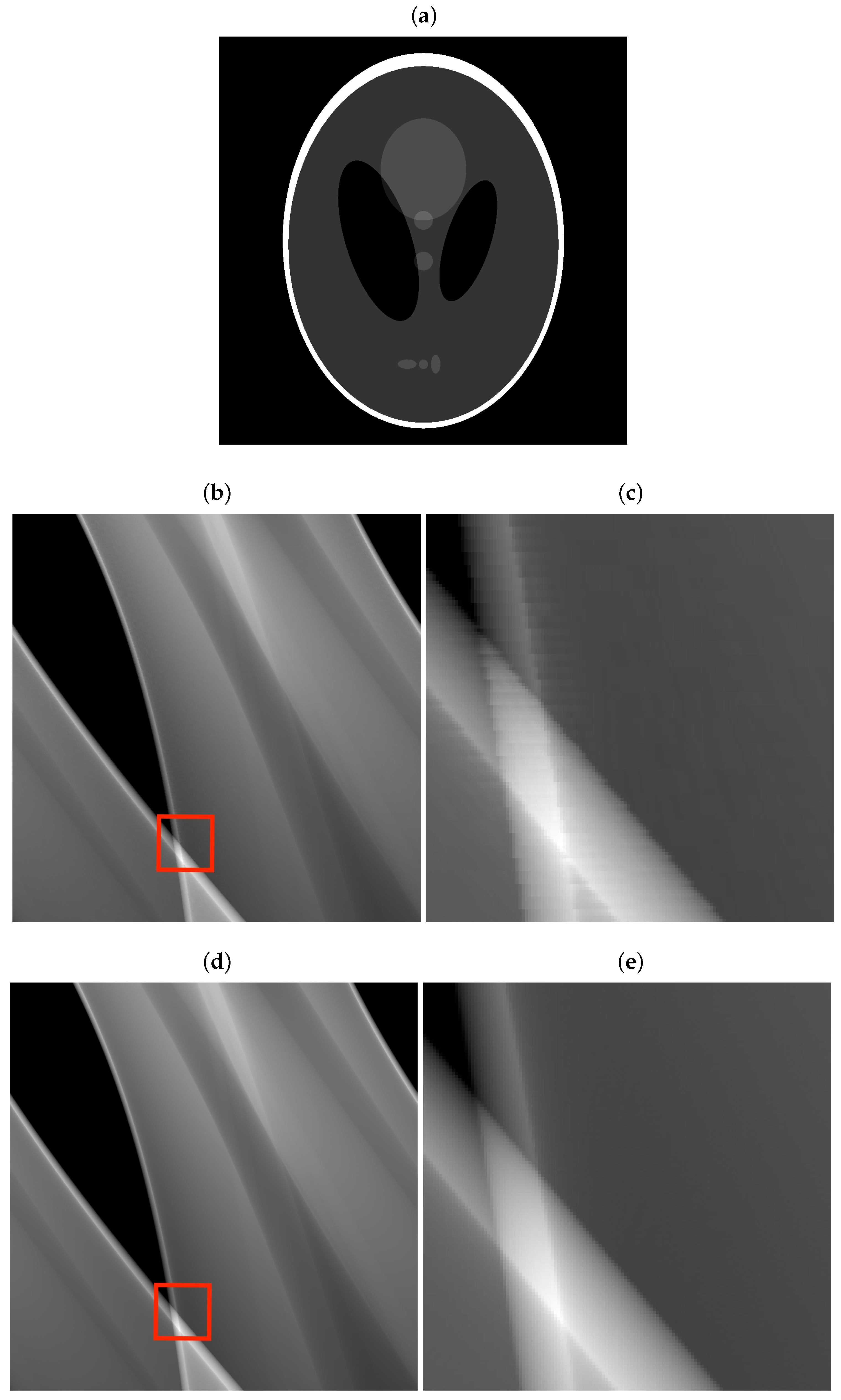
Figure 6 illustrates the impact of geometric approximation errors on the values of the Hough image. The test image is the Shepp–Logan phantom [65], with a resolution of $4096\times 4096$ pixels. When constructing the Hough image using the Brady–Yong algorithm, noticeable high-frequency artifacts are observed. Conversely, these artifacts are absent when employing the DSLS patterns.

5.4. Final Touches

With the aforementioned constraints, the $ASD2$ algorithm has a complexity of $O\left(w^{5/3}h\right)$ when processing an image of size $w\times h$. It computes the sums over the patterns from the set $S_{w,h}^{KCH+}\subset S_{w,h}^{CH+}$, while initially, we were faced with the task of summing over patterns from $S_{w,h}$. In Section 4, we decided to limit ourselves to a smaller number of patterns, which we referred to as key patterns.

Let us define the key patterns from the set $S_{w,h}$:

$$\begin{array}{cc}\hfill & S_{w,h}^K\stackrel{\mathrm{def}}{=}{S}_{w,h}^{KH}\cup S_{w,h}^{KV},\hfill \\ \hfill & S_{w,h}^{KH}\stackrel{\mathrm{def}}{=}\left\{p=p_{w,h}^H\left(\frac{k_z}{w-1},b\right)|k_z\in (-w+1,w-1]\subset \mathbb{Z}\wedge b\in \mathbb{Z}\wedge p\ne \varnothing \right\},\hfill \\ \hfill & S_{w,h}^{KV}\stackrel{\mathrm{def}}{=}\left\{p=p_{w,h}^V\left(\frac{k_z}{h-1},b\right)|k_z\in [-h+1,h-1)\subset \mathbb{Z}\wedge b\in \mathbb{Z}\wedge p\ne \varnothing \right\}.\hfill \end{array}$$

(23)

The procedure for calculating sums over patterns from the set $S_{w,h}^K$ in the image $I_{w,h}$ using the $ASD2$ algorithm completely repeats the scheme of applying the Brady–Yong algorithm [1].

The image ($I_{w,h}$) is padded with zeros up to a size of $I_{w,h+w}$. The $ASD2$ algorithm is applied to this image. The same pair of operations is performed with the image reflected on the second axis, the transposed image, and the transposed and reflected image. The resulting four sets of sums cover the set $S_{w,h}^K$. The total complexity of the algorithm in this case is $O(w^{8/3}+h^{8/3})$.

6. Discussion

The $Build\_Gkchp$ function in the $ASD2$ algorithm can be replaced without affecting its functionality. Thus, the list of patterns to be summed can be varied. This is interesting both in terms of further introduction of sparsity into the pattern set in cases when high-resolution results are not required and in terms of computing patterns with $k\le 0$ and with $k\ge 0$ in a single pass. The computational complexity of such modifications to the $ASD2$ algorithm is not discussed in this work. However, it is clear that for majorization of summations, the $AS4R$ algorithm relies not on the internal structure of the pattern set but only on its cardinality.

It is also worth noting that the $ASD2$ algorithm itself does not require the condition $w=8^q$ to be satisfied, as this condition is used only to construct a complexity estimate. As for the original Brady–Yong algorithm, its modification supporting arbitrary array sizes was published only in 2021 [66]. A solution to this problem had already been announced nine years earlier in [67], but the proposed algorithm was based on factoring of the array size and was not efficient for sizes with large prime factors. As for the $ASD2$ algorithm, it would be interesting to evaluate its complexity for arbitrary image sizes.

It is also interesting to consider the generalization of the $ASD2$ algorithm to three-dimensional images. Generalizations of the Brady–Yong algorithm for summations over lines and planes in three-dimensional images were first published by T.-K. Wu and M. Brady in 1998 [68], but this publication in the proceedings of a symposium on image processing and character recognition went unnoticed for a long time. Both algorithms have been repeatedly reinvented [26,69].

It is worth noting that the estimation of the number of DSLS in this work is not the first of its kind. A more accurate estimation was obtained in [70], but the reasoning presented in Section 3.2 appears to be simpler to us while still illustrating one of the key ideas of the paper.

Another important area for future research is the numerical comparison of the various algorithms investigated in this study, including the Brady–Yong and Khanipov algorithms. To conduct such a comparison, it is necessary to reconstruct the Khanipov algorithm based on the provided scheme. Ensuring a fair assessment under identical conditions requires the careful implementation of all algorithms. It is particularly important to pay attention to algorithms based on the pseudo-polar Fourier transform, as their performance can be significantly influenced by the choice of libraries. Additionally, it would be interesting to compare the accuracy of these algorithm classes using a fixed data discretization model.

Finally, in certain applications, such as tomographic reconstruction, it is necessary to obtain not the projection operator (A) calculated by the aforementioned algorithms but its “inverse”. The use of quotation marks in this context is to highlight that in reconstruction problems, a regularized problem is typically stated:

$${\parallel Ax-y\parallel }^2+R\left(x\right)\to \underset{x}{min},$$

(24)

where x is the target image, y is the observed image, and R is a regularizer. One approach to tackle this optimization problem involves gradient-descent-type iterative algorithms [71]. These algorithms require repeated computations of the adjoint operator ($A^T$). From this perspective, fast algorithms for computing the adjoint operator of the Hough transform are more significant than fast algorithms for direct inverse transform. It is feasible to modify the considered algorithms to efficiently compute the image $A^{T}z$, and this aspect warrants further research.