A Joint Optimization Algorithm Based on the Optimal Shape Parameter–Gaussian Radial Basis Function Surrogate Model and Its Application

Abstract

We propose a joint optimization algorithm that combines the optimal shape parameter–Gaussian radial basis function (G-RBF) surrogate model with global and local optimization techniques to improve accuracy and reduce costs. We analyze factors that affect the accuracy of the G-RBF surrogate model and use the particle swarm optimization (PSO) algorithm to determine the optimal shape parameter and control the number and spacing of the sampling points for a high-precision surrogate model. Global optimization refines the surrogate model, serving as the initial value for local optimization to further refine the problem. Our experiments show that this method significantly reduces computation costs. We optimize the section size of cantilever beams for different materials, obtaining the optimal section size and mass for each. We find that hard aluminum alloy is the optimal choice, meeting yield strength and deflection requirements through finite element analysis verification. Our work highlights the effectiveness of the joint optimization algorithm based on the surrogate model, providing valuable tools and insights into optimizing various structures.

1. Introduction

In practical systems, physical models may be insufficient to describe system behavior due to external factors and error terms. Response surface methodology (RSM) [1] is a modeling approach that explores nonlinear relationships between input and output variables and models, predicts, and optimizes the objective function. However, the objective function is often complex, nonlinear, and difficult to solve using analytical methods. Therefore, constructing a response surface model that approximates the objective function using experimental data can help engineers and scientists better understand practical systems, predict unknown behavior, and make scientific decisions. Different methods can be used to construct response surface models, including polynomial regression, moving least squares, Kriging, and radial basis function (RBF) methods. Polynomial regression [2] is simple and easy to use and can handle most nonlinear problems but can face difficulties in addressing high-dimensional problems. Moving least squares (MLS) [3] is simple in form and computationally efficient but it has poor approximation ability for nonlinear models. Kriging [4] is a widely used approximation method for handling linear and nonlinear problems with high prediction accuracy, but it has high computational costs and is unsuitable for discrete output variables. RBF [5] has several advantages, including a simple form, isotropy, dimension independence, and suitability for high-dimensional problems. This paper adopts the G-RBF as the approximation function to construct a high-precision surrogate model. The selection of shape parameters directly affects the interpolation effect when using the G-RBF for interpolation [6,7,8]. Nevertheless, the selection of shape parameters is mostly achieved using trial-and-error or empirical methods, resulting in low efficiency or accuracy. Hence, this paper employs the particle swarm algorithm to select the shape parameters for test functions of different dimensions. Comparative experiments are performed to verify that the selected shape parameters can achieve high interpolation accuracy.

In the field of multidisciplinary design optimization, direct optimization utilizing high-precision models becomes infeasible when the complexity of the models expands. Frequently, a response surface model is created as a low-precision model to iteratively optimize and decrease the frequency at which the high-precision model is executed, ultimately decreasing expenses. Although some approaches can enhance the precision of the approximate model, they may not be as effective in reducing the high-precision model’s frequency of execution. In contrast, techniques that incorporate optimized solutions into the approximate model could cause the approximate model to converge locally and lose global optimality [9,10]. Our proposed method aims to regulate the number of times the high-precision model is run during the model approximation process. In particular, our global optimization method optimizes the approximate model’s solution and utilizes it as the starting point for the local optimization of the high-precision model. This guarantees that the solution will be valid within the feasible domain. The global optimization method’s ability to search on a global scale enables it to discover superior initial conditions, whereas the quick convergence rate of the local optimization method can minimize the high-precision model’s frequency of execution and guarantee solution reliability. Experimental testing provides verification of the efficacy of the joint optimization algorithm.

Cantilever beams are extensively used in the automatic feeding devices of single-machine multi-station stamping systems and their structural parameters require optimized designs to ensure higher stability and economic benefits under specific working conditions [11]. However, the choice of optimization methods significantly impacts the final optimization results. Although numerical optimization methods such as the gradient method, simplex method, and direct search method are highly efficient, they often yield locally optimal solutions, making it challenging to achieve a globally optimal solution [12,13,14]. On the other hand, optimization methods like colony optimization and the genetic algorithm possess good global optimization capabilities but come with high computational costs [15,16]. This study proposes a joint optimization algorithm based on the G-RBF surrogate model with optimal shape parameters to achieve the lightest weight of the cantilever beam structure of automatic feeding devices. Our algorithm achieves a globally optimal solution while significantly reducing the frequency of high-precision model calls, thus saving computational costs. Our work contributes to material design by providing a practical and efficient optimization approach for cantilever beam structures in automatic feeding devices, which can enhance their stability and economic benefits under specific working conditions.

2. G-RBF Surrogate Model

2.1. G-RBF Interpolation Principle

The radial basis function consists of a weighted sum of radial basis functions centered at different points in the input space. In our study, we used a Gaussian radial basis function, and the centers were chosen to be the training samples. The weights of the radial basis functions were determined by solving a linear system of equations that enforced the interpolation or approximation of the training data. This expression is shown below [7]:

$$\stackrel{\sim }{y}=\sum _{k=1}^n{\omega }_k\left({\varphi }_k\left(∥x-x_k∥\right)\right)=W^{{}^T}\Phi \left(x\right)$$

(1)

The weight coefficient vector, represented by $W={\left[{\omega }_1,{\omega }_2,\dots ,{\omega }_n\right]}^T$, can be calculated using the following formula:

$$W=A^{-1}y$$

(2)

Matrix A can be computed using the following formula:

$$A=\left[\begin{array}{ccc}\phi \left(∥x_1-x_1∥\right)& \cdots & \phi \left(∥x_1-x_n∥\right)\\ ⋮& \ddots & ⋮\\ \phi \left(∥x_n-x_1∥\right)& \cdots & \phi \left(∥x_n-x_n∥\right)\end{array}\right]$$

(3)

where $\phi \left(\left|x-x_1\right|\right)$ is a radial basis function. A common choice for $\phi$ is the Gaussian radial basis function (G-RBF), which can be expressed as follows:

$$\phi \left(r\right)={\mathrm{e}}^{-c^2{r}^2}$$

(4)

In Equation (4), c is the shape parameter of the Gaussian radial basis function.

In two-dimensional space, the G-RBF can be expressed as [17]:

$$Gauss=exp\left[-\frac{{\left(x-\mu x\right)}^2}{2{\delta x}^2}-\frac{{\left(y-\mu y\right)}^2}{2{\delta y}^2}\right]$$

(5)

In three-dimensional space, the Gaussian radial basis function can be expressed as [17]:

$$Gauss=exp\left[-\frac{{\left(x-\mu x\right)}^2}{2\delta x^2}-\frac{{\left(y-\mu y\right)}^2}{2\delta y^2}-\frac{{\left(z-\mu z\right)}^2}{2\delta z^2}\right]$$

(6)

In Equations (5) and (6), $\left(x,y,z\right)$ is the coordinate of the center of the grid; $({\mu }_x,{\mu }_y,{\mu }_z)$ is the center coordinate of the radial basis function; and ${\delta }_x$, ${\delta }_y$, and ${\delta }_z$ are the distribution radii of the radial basis function. The radial basis function is used to approximate the underlying function of the dataset, which enables us to make predictions for new, unseen data points. By using the radial basis function, we are able to capture the nonlinear relationships between the input variables and the output variable, which cannot be achieved with linear models.

2.2. Factors Affecting the Effectiveness of the G-RBF Surrogate Model

There are two main factors that impact the G-RBF interpolation effect, which are as follows [7]:

• Shape parameter:

The Gaussian radial basis function (G-RBF) interpolation method has been widely used in various fields due to its high accuracy and efficiency. However, the choice of the shape parameter, c, is critical to the success of the G-RBF interpolation, as it directly affects the shape of the basis function. As shown in Figure 1, different values of c can result in significantly different shapes of the G-RBF. Furthermore, an optimal value of c, denoted as $c_{opt}$, exists for each unique interpolation problem, which can greatly improve the accuracy of the interpolation results.

To demonstrate the importance of selecting an appropriate value for c, we conducted an experiment on the interpolation of Equation (16) using the G-RBF method with different values of c. As shown in Figure 2, the interpolation error is highly dependent on the choice of c, with an optimal value of $c_{opt}$ that minimizes the interpolation error. These findings are consistent with previous studies, highlighting the critical role played by the shape parameter c in the G-RBF interpolation method.

Therefore, selecting an appropriate shape parameter c is crucial for obtaining accurate and reliable G-RBF interpolation results. Future studies could explore robust methods for determining the optimal value of c in various interpolation problems and further investigate the performance of the G-RBF interpolation method in different applications.

• Conditional number:

Determining the value of $A^{-1}$ in Equation (16) is crucial for obtaining the interpolation function. Although A is non-singular when the sampling points are dissimilar, its condition number can become exceedingly large. The condition number of A is defined as

$$condA=\left|A^{-1}\right|·\left|A\right|$$

(7)

To calculate $condA$, one needs to evaluate $\lambda max$ and $\lambda min$, which are the maximum and minimum eigenvalues of A. The formula is given by

$$condA=\left|\lambda \max /\lambda \min \right|$$

(8)

When the sampling points are near, A is a matrix that is often considered poorly conditioned. Figure 3 illustrates the relationship between the matrix condition number and the number of sampling points used for the G-RBF interpolation of Equation (16). It can be observed that as the number and distribution of the sampling points increase, the matrix condition number becomes more ill-conditioned. The problem posed by a poorly conditioned matrix is that imperfections in the solution of linear equations can significantly affect the precision of the approximation.

Generally, there are two approaches to handling a poorly conditioned matrix: improving the distance between the sampling points or utilizing a more precise equation. However, increasing the number of sampling points can exacerbate the equation-solving challenge to the extent that an accurate solution becomes practically unattainable, greatly impairing model accuracy.

With regard to the two main factors that affect the G-RBF interpolation effect mentioned above, we appropriately set them in Section 2.3.1 and Section 2.4, respectively. This results in a high-precision G-RBF surrogate model.

2.3. Optimal Shape Parameter Determination in G-RBF Interpolation

2.3.1. Optimal Shape Parameter Determination Based on Particle Swarm Optimization in G-RBF Interpolation

The selection of the shape parameters in G-RBF interpolation can be transformed into the following optimization problem:

$$E_{max}\left(c\right)=\underset{x\in \left(a,b\right)}{max}|s\left(x,c\right)-f\left(x\right)|$$

(9)

$$\left\{\begin{array}{cc}\hfill & Find{c}_{opt}\hfill \\ \hfill & min{E}_{max}\left(c\right)\hfill \end{array}\right.$$

(10)

The parameters of the interpolation include the interpolation basis function $s\left(x,c\right)$, the primitive function $f\left(x\right)$, the maximum error $E_{max}\left(c\right)$, and the required optimal shape parameter $c_{opt}$ for the interpolation.

Particle swarm optimization (PSO) [18] is a population-based optimization algorithm inspired by the social behavior of birds. PSO maintains a population of particles, each representing a potential solution to the optimization problem. Each particle has a position and velocity in the search space, and the algorithm updates these values iteratively to search for the optimal solution.

The position of each particle at iteration t is represented by a vector $x_i\left(t\right)$, and its velocity is represented by a vector $v_i\left(t\right)$. The best position that particle i has achieved so far is denoted by $p_i\left(t\right)$, and the best position achieved by any particle in the swarm is denoted by $g\left(t\right)$. The objective function to be optimized is denoted by $f\left(x\right)$.

At each iteration, the algorithm updates the position and velocity of each particle based on its current position, velocity, and the best positions achieved by both itself and the swarm as a whole. The position and velocity updates are given by:

$$v_i(t+1)=w{v}_i\left(t\right)+c_1{r}_1(p_i\left(t\right)-x_i\left(t\right))+c_2{r}_2(g\left(t\right)-x_i\left(t\right))$$

(11)

$$x_i(t+1)=x_i\left(t\right)+v_i(t+1)$$

(12)

where w is the inertia weight, which controls the particle’s tendency to maintain its current velocity. $c_1$ and $c_2$ are the cognitive and social learning factors, respectively, which control the particle’s tendency to follow its personal best position and the swarm’s best position. $r_1$ and $r_2$ are random numbers drawn from a uniform distribution.

The algorithm terminates when a stopping criterion, such as a maximum number of iterations or a desired level of convergence, is met. The best solution found by the algorithm is the particle with the best position achieved throughout the iterations.

In summary, PSO is a population-based optimization algorithm that updates the position and velocity of each particle based on its current position, velocity, and the best positions achieved by both itself and the swarm as a whole. By emulating the social behavior of birds, PSO is capable of efficiently searching for the optimal solution to complex optimization problems.

This paper employs PSO to optimize the shape parameters of G-RBF interpolation. This technique is particularly advantageous when dealing with complex systems that have a large amount of data to model using the G-RBF proxy. It provides a significant time reduction for parameter determination. G-RBF interpolation requires the determination of the optimal shape parameter $c_{opt}$ to minimize the interpolation error. The process is as follows:

Step 1: Initialize the particle swarm

Assuming that the particle swarm consists of n particles, the position and velocity of each particle can be denoted by $x_i$ and $v_i$, respectively. The initial position and velocity are generated randomly and typically follow a uniform or Gaussian distribution.

Step 2: Determine the fitness value.

The position of each particle represents a viable design solution. Based on the current position, the objective function value indicated by the maximum absolute error is used as the particle’s fitness value $f_i$.

Step 3: Update particle speed and position.

The velocity ($v_{it}$) and position ($x_{it}$) of the particles are updated during the t-th iteration as follows:

$$v_{it}=w{v}_{it}+c_1{r}_1(x_{pbesti}-x_{it})+c_2{r}_2(x_{gbest}-x_{it})$$

(13)

$$x_{it+1}=x_{it}+v_{it}$$

(14)

Here, the inertia weight (w) regulates the particle motion’s inertia. The acceleration coefficients ($c_1$ and $c_2$) determine the impact of the particle’s individual historical best position ($x_{pbesti}$) and the global best position ($x_{gbest}$) on the particle’s velocity. The random numbers ($r_1$ and $r_2$) create a stochastic element in the calculation.

Step 4: Update the optimal value

Following each iteration, the historical and globally optimal values of every particle are updated. For the ith particle, if the current position generates a fitness value $f_i$, which is less than its historical optimal fitness value $f_{pbes{t}_i}$, $pbes{t}_i=x_i$ and $f_{pbes{t}_i}=f_i$ will be updated. $gbest$ is updated with the position that has the lowest fitness value among all particles.

Step 5: Convergence Judgment

It is determined whether the particle swarm has converged, meaning that the position of the particle has barely changed or not changed at all. If the iteration stop condition is met, the globally optimal value and position are output. Consequently, the algorithm ends. If not, the algorithm returns to Step 3 for another iteration. To ensure the reproducibility of our results, we have provided detailed information on the specific parameters and settings used in the PSO algorithm. The PSO algorithm was used to optimize the shape parameter and manage the sampling points. The swarm size was set to 50, the maximum number of iterations was set to 500, the inertia weight was set to 0.8, and the cognitive and social parameters were set to 1.5. The constriction factor was set to 0.729 to ensure the convergence of the algorithm.

In conclusion, the PSO algorithm outputs the optimal shape parameter $c_{opt}$ of the G-RBF based on the calculated results. Following experimental research by numerous researchers [19,20,21,22,23,24,25,26], it has been confirmed that the method proposed in [27] demonstrates high accuracy in selecting the shape parameters of radial basis function interpolation. Therefore, it has been widely utilized. In this section, this study selected seven test functions from [27,28,29] (

Table 1. Test functions.

f
$f_1=\frac{x^2}{8+x^5}$
$f_2=0.75exp\left(-\frac{{\left(9x-2\right)}^2+{\left(9y-2\right)}^2}{4}\right)+0.75exp\left(-\frac{{\left(9x+1\right)}^2}{49}+\frac{9y+1}{10}\right)$
$+0.5exp\left(-\frac{{\left(9x-7\right)}^2+{\left(9y-3\right)}^2}{4}\right)-0.2exp\left(-{\left(9x-4\right)}^2-{\left(9y-7\right)}^2\right)$
$f_3=\frac{tanh\left(9y-9x\right)+1}{9}$
$f_4=\frac{1.25+cos\left(5.4y\right)}{6\left(1+{\left(3x-1\right)}^2\right)}$
$f_5={\displaystyle \sum _{i=1}^5}\left[\frac{3}{10}+sin\left(\frac{16}{15}{x}_i-1\right)+{sin}^2\left(\frac{16}{15}{x}_i-1\right)\right]$
$f_6={\displaystyle \sum _{i=1}^{10}}{x}_i(1+ln\frac{x_i}{x_i+x_{10}})$

and

Table 2. Parameter setting.

f	Vars.	Design Domain	Sample Points
$f_1$	1	$x\in \left[0,7\right]$	21
$f_2$	2	$x\in \left[0,1\right],y\in \left[0,1\right]$	1000
$f_3$	2	$x\in \left[0,1\right],y\in \left[0,1\right]$	1000
$f_4$	2	$x\in \left[0,1\right],y\in \left[0,1\right]$	1000
$f_5$	5	$x_i\in \left[-1,1\right]$	80
$f_6$	10	$x_i\in \left[0.5,10\right]$	200

) and calculated them under the same conditions specified in Section 2.3.1, comparing the experimental results to those obtained using the method in [27] (

Table 3. Comparison with the effect of the method in [27].

f	${\mathit{c}}_{\mathit{opt}}$		RMSE		Operation Time(s)
	PSO	[27]	PSO	[27]	PSO	[27]
$f_1$	0.333	0.392	$1.23\times {10}^{-2}$	$1.41\times {10}^{-2}$	0.015	1.601
$f_2$	0.172	0.188	$2.01\times {10}^{-3}$	$2.55\times {10}^{-3}$	0.226	2.279
$f_3$	1.327	1.0878	$4.23\times {10}^{-3}$	$5.33\times {10}^{-3}$	1.439	3.763
$f_4$	0.356	0.8465	$1.96\times {10}^{-4}$	$7.45\times {10}^{-4}$	3.014	7.419
$f_5$	0.012	0.625	$7.82\times {10}^{-3}$	$6.84\times {10}^{-2}$	10.812	39.726
$f_6$	0.714	1.826	$1.71\times {10}^{-2}$	$5.92\times {10}^{-2}$	1.171	3.365

).

Based on the experimental results in Table 3, the PSO algorithm was found to be effective in determining the optimal shape parameters of G-RBF interpolation. Specifically, our method significantly reduced the operational cost and improved the accuracy of interpolation, particularly for $f_5$.

2.4. Control of Sampling Points

Section 2.2 examines how sampling points affect the accuracy of the G-RBF surrogate model, and we regulate it with regard to the selection, number, and spacing of sampling points.

First of all, the selection of sampling points is a crucial step in the research methodology and must be carried out according to specific principles. It is imperative that the sampling points chosen for this study are representative of the entire space, as the accuracy of the approximate model heavily relies on this factor. Given the unique properties of the Latin hypercube method [30], it is the preferred approach for extracting information from the entire space and is therefore utilized in this study.

Moreover, the addition of sample points needs to be regulated. Once the model attains a specific accuracy level, there is no need to continue adding sample points. Here is the particular regulation method: the accuracy threshold is established as $\theta$ for the proxy model. If the root mean square error (RMSE) is less than $\theta$, there is a need to increase the sample point. On the other hand, it is unnecessary to add sample points if the RMSE is greater than or equal to $\theta$. Moreover, the number of sampling times is restricted to a maximum value of N.

Finally, it is critical to regulate the spacing between sampling points. As described in Section 2.2, having sampling points that are too close may result in an ill-conditioned matrix A, hence the need to regulate the spacing between added points. In some cases, it is also essential to ensure that the distance between points is not too close since, at times, this could inadequately represent the system’s entire information, thus negatively affecting the global optimization outcomes. Moreover, a program may end too early when an addition point is too close to an existing sampling point, thus failing to meet the precision requirements. As a result, it is crucial to filter and remove points that are too close after adding them. The current sampling points are labeled as $S_e=\left\{x_1,\dots ,x_j,\dots ,x_s\right\}$. The collection of points added after them is marked as $S_a=\left\{x_1,\dots ,x_i,\dots ,x_n\right\}$. Since the shape parameter c mainly determines matrix element values and plays a significant role in assessing points’ proximity degree, the criterion for governing sampling point spacing, after the determination of $c_{opt}$ using the method described in Section 2.3.1, is whether $d_i=∥x_i-x_j∥>c_{opt}$ satisfies a specific condition for each $x_i$ in $s_a$.

3. Joint Optimization Algorithm Based on G-RBF Surrogate Model

3.1. Main Idea of the Joint Optimization Algorithm

One of the key advantages of global optimization algorithms is their ability to escape the limitations of locally optimal solutions. Although they possess strong search capabilities, their convergence speed is relatively slow, necessitating multiple high-precision model calculations. Alternatively, local optimization methods demonstrate faster convergence rates but are prone to reaching locally optimal solutions, particularly when a poor initial value is selected. In response to these issues, the joint optimization method utilizes the global search capabilities of the former coupled with the faster convergence rate of the latter to ensure optimization convergence, minimize high-precision model calculations, and reduce calculation costs.

Initially, data are utilized to determine the optimal shape parameters using the method described in Section 2.3.1. Then, a surrogate model using G-RBF is constructed. Subsequently, the global optimization method is used to optimize the model, with the optimization cost being very small due to the simplicity of the G-RBF surrogate model. Lastly, the optimized variable value is taken as the initial value, and a local optimization algorithm is subsequently used to optimize the high-precision surrogate model to ensure the accuracy of the optimized solution.

3.2. Process of the Joint Optimization Algorithm

This section first provides specific details regarding the control thresholds for various parameters and the error evaluation method for the joint optimization process. The accuracy threshold for the surrogate model is represented by $\theta$, the maximum number of sampling times is N, and the inter-sample distance is controlled by $copt$. The evaluation of errors is computed using the root-mean-square-error (RMSE) method expressed as:

$$RMSE=\sqrt{\frac{{\displaystyle \sum _{i=1}^N}\left(y_i-{\tilde{y}}_i\right)}{N}}$$

(15)

The following section outlines the specific steps involved in the joint optimization algorithm based on the G-RBF surrogate model with an optimal shape parameter.

Step 1: The entire system is sampled using Latin hypercube, followed by the selection of the optimal shape parameters based on the sampling points using the method described in Section 2.3.1.

Step 2: The surrogate model undergoes precision verification, where the existence of $RMSE>\theta$ warrants the further addition of points. According to the description in Section 2.4, validation procedures are necessary for each addition. Newly added point $x_i$ must satisfy the condition $d_i=∥x_i-x_j∥>c_{opt}$ relative to the preexisting point $x_j$. Thus, the addition of each point is either valid or invalid, and the invalid point must be re-added until $RMSE<\theta$ is achieved or the maximum number of sampling times reaches N.

Step 3: The G-RBF surrogate model obtained can be optimized using global optimization techniques to determine the optimal solution. The use of a sampling strategy that ensures that points are well spaced allows the surrogate model to represent global information. Therefore, the optimal solution obtained through global optimization techniques is likely to be very close to the optimal solution of the original problem.

Step 4: The global optimization solution serves as an initial value submitted to the local optimization method to further optimize the high-precision G-RBF surrogate model, resulting in the optimal solution of the joint optimization algorithm.

The joint optimization algorithm is presented in the form of a flowchart in Figure 4.

3.3. Testing the Joint Optimization Algorithm

In this section, we test the effectiveness of the G-RBF surrogate-based joint optimization algorithm using two two-dimensional test functions. In practical applications, it is important to avoid excessive calls to high-precision models. Therefore, when comparing the global optimization algorithm, local optimization algorithm, and joint optimization algorithm, the maximum absolute error (MaxError) was chosen as the measure of error for the design variables. The MaxError in function values ($E_y$), the MaxError in variable values ($E_x$), and the number of G-RBF surrogate model calls (T) are compared.

• Test case 1: Ackley Function

The Ackley Function [31] is a multimodal function with multiple local minima and a very complex landscape. It is defined as follows:

$$f(x,y)=-20exp\left(-0.2\sqrt{\frac{1}{2}(x^2+y^2)}\right)-exp\left(\frac{1}{2}[cos\left(2\pi x\right)+cos\left(2\pi y\right)]\right)+e+20$$

(16)

Here, x and y are the independent variables that lie in the range $-5\le x,y\le 5$.

The optimal solution and value refer to the minimum point and value, respectively, of the function. The optimal solution for the Ackley Function is $(0,0)$, where the function reaches its minimum value of $f(0,0)=0$. Optimization algorithms can be employed to find the optimal solution. This study employed a genetic algorithm as the global optimization algorithm and a gradient descent method as the local optimization algorithm.

A genetic algorithm (GA) is a population-based optimization algorithm that mimics the process of natural selection to search for the optimal solution. The algorithm maintains a population of candidate solutions, represented by a set of chromosomes, and iteratively applies genetic operators, such as selection, crossover, and mutation, to generate new offspring. The fitness of each individual is evaluated based on the objective function, and the population evolves toward better solutions over time. The GA terminates when a stopping criterion, such as a maximum number of generations, is met or when the optimal solution is found.

The gradient descent method is an iterative optimization algorithm that seeks to minimize a function by iteratively adjusting the parameters in the direction of the negative gradient of the function. At each iteration, the algorithm computes the gradient of the function with respect to the current parameter values and updates the parameters in the direction of the negative gradient. The step size of the update is controlled by a learning rate parameter, which determines the size of the step taken in each iteration. The algorithm terminates when a stopping criterion, such as a desired level of convergence or a maximum number of iterations, is met.

In this study, the GA was employed as the global optimization algorithm to search for the optimal set of design variables, whereas the gradient descent method was used as the local optimization algorithm to refine the solution obtained using the GA. Specifically, the GA was used to generate a set of candidate solutions, and the best solution was selected as the initial point for the gradient descent method. The gradient descent method was then employed to fine-tune the solution by iteratively adjusting the design variables in the direction of the negative gradient of the objective function. The process was repeated until convergence was achieved or a maximum number of iterations was reached.

In summary, the combination of the genetic algorithm and gradient descent method allowed for efficient global and local optimization, respectively, and enabled the algorithm to search for the optimal solution in a large search space. A population size of 30 and 100 generations was used. The initial values for the gradient descent method were set to [−5, 0].

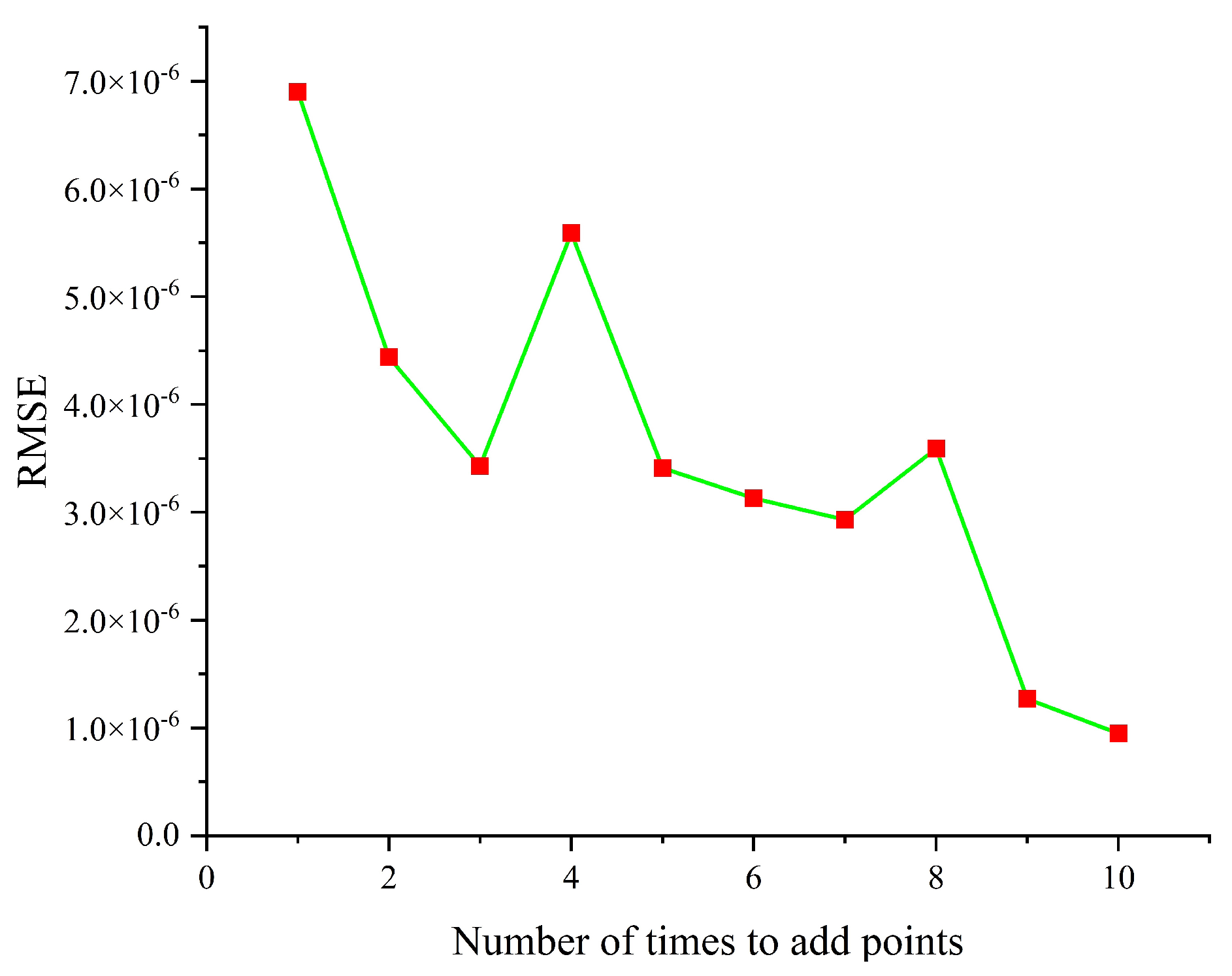
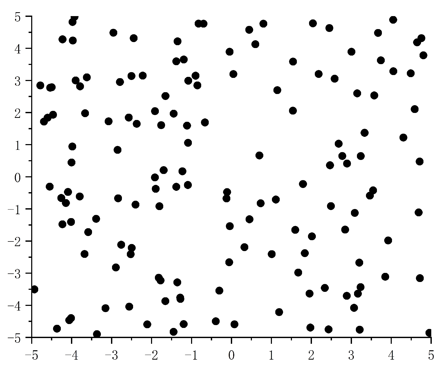
The best shape parameter $c_{opt}=1.668$ for the G-RBF interpolation of (16) was determined using the method described in Section 2.3.1. The RMSE threshold for the surrogate model was set to $\theta =1\times {10}^{-6}$, and Figure 5 and Figure 6 show the RMSE of the G-RBF surrogate model and the distribution of sampled points.

The distribution of the sampling points, including the added points, appeared to be fairly uniform across the global range. This suggests that the controlled refinement strategy in Section 2.4 was effective in ensuring that the surrogate model adequately captured the global characteristics. This ensures that our joint optimization algorithm can find the global optimal solution.

The convergence of the genetic algorithm optimization of the original objective function and our proposed joint optimization algorithm are compared in Figure 7 and Figure 8.

Table 4. Comparison of optimization methods for the objective function (16).

Algorithm	${\mathit{E}}_{\mathit{y}}$	${\mathit{E}}_{\mathit{x}}$	T
Genetic	$1\times {10}^{-6}$	$1\times {10}^{-6}$	1038
gradient descent	$3.3\times {10}^{-2}$	$5.8\times {10}^{-1}$	560
Joint optimization	$1\times {10}^{-6}$	$1\times {10}^{-6}$	170

compares the optimization error and the number of function evaluations for the objective function (16).

As the gradient descent method exhibited significantly larger errors compared to the other two algorithms, we do not discuss it in detail here. In contrast, both the genetic algorithm and joint optimization methods converged to the exact solution, as demonstrated in Figure 7 and Figure 8 and Table 4. However, there were differences in their convergence behaviors. The joint optimization method converged more swiftly to the vicinity of the exact solution during the iteration thanks to decent initial values. In contrast, the genetic algorithm required considerably more operations of the high-fidelity G-RBF surrogate model before converging to the solution. These results highlight the effectiveness of the joint optimization method in reducing computation costs and accelerating convergence while ensuring solution accuracy.

• Test case 2: Rosenbrock’s Banana Function

Rosenbrock’s Banana Function [32] is a well-known constrained optimization problem, which is frequently utilized for evaluating optimization algorithms’ performance. The function can be formulated as minimizing the Equation:

$$f(x,y)={(1-x)}^2+100{(y-x^2)}^2,x+y\le 2$$

(17)

where x and y are bounded by the range $[-2,2]$. The optimal solution to this problem is achieved when $x=1$ and $y=1$, at which point the objective function attains the minimum value of $f(x,y)=0$. We employed the ant colony algorithm as our global optimization method and the simplex method as the local optimization in our study.

The ant colony algorithm (ACA) is a metaheuristic optimization algorithm inspired by the behavior of ants in finding the shortest path between their colony and food sources. The algorithm maintains a set of artificial ants, each representing a potential solution to the optimization problem. The ants construct a pheromone trail based on the quality of the solutions they encounter, and the pheromone trail guides subsequent ants toward better solutions. The algorithm terminates when a stopping criterion, such as a maximum number of iterations or a desired level of convergence, is met. The best solution found by the algorithm is the one with the highest pheromone trail.

The simplex method is an iterative optimization algorithm that seeks to minimize a linear objective function subject to linear constraints. The algorithm starts with a feasible solution and iteratively moves toward the optimal solution by adjusting the variables within the constraints. At each iteration, the algorithm identifies a non-basic variable that can improve the objective function value and moves along the direction of the corresponding constraint boundary until a new basic feasible solution is found. The algorithm terminates when a stopping criterion, such as a desired level of convergence or a maximum number of iterations, is met.

In this study, we employed the ACA as the global optimization algorithm and the simplex method as the local optimization method. Specifically, the ACA was used to explore the search space and identify promising regions for the optimization problem. The best solution found by the ACA was then used as the initial point for the simplex method, which iteratively improved the solution by adjusting the design variables within the constraints. The process was repeated until convergence was achieved or a maximum number of iterations was reached.

In summary, the combination of the ant colony algorithm and simplex method allowed for efficient global and local optimization, respectively, and enabled the algorithm to search for the optimal solution in a large search space subject to linear constraints.

The optimal parameter is $c_{opt}=1.001$, with an RMSE threshold of $\theta =1\times {10}^{-6}$. Figure 9 and Figure 10 illustrate the convergence process of the ant colony and joint optimization algorithms.

Table 5. Comparison of optimization algorithms for the objective function (17).

Algorithm	${\mathit{E}}_{\mathit{y}}$	${\mathit{E}}_{\mathit{x}}$	T
Ant Colony	$1\times {10}^{-6}$	$1\times {10}^{-6}$	1945
Simplex	$8.9\times {10}^{-1}$	$3.2\times {10}^{-1}$	661
Joint optimization	$1\times {10}^{-6}$	$1\times {10}^{-6}$	382

compares the results obtained using the three optimization algorithms.

The solution obtained using the simplex method was far from optimal so we do not discuss this in detail here. Table 5 and Figure 9 and Figure 10 show that both the ant colony and joint optimization algorithms converged to the optimal solution. It should be noted that the joint optimization algorithm needs to run the Gaussian radial basis function surrogate model only one-fifth of the times required by the ant colony algorithm. This further supports the effectiveness of the algorithm proposed in this study.

3.4. Feasibility of the Joint Optimization Algorithm

Our joint optimization algorithm employs three technologies: a high-precision G-RBF surrogate model with an optimal shape parameter, global optimization, and local optimization. In order to ensure uniformity in space, express the whole-space characteristics, and bring the solution of the global optimization algorithm closer to the actual solution, the control-plus-point strategy is employed in the sampling distribution. The convergence of the method is guaranteed by the existing global optimization algorithms. Hence, the joint optimization algorithm is deemed feasible.

From the two classic test functions, it is evident that the joint optimization algorithm can efficiently attain global optimization goals. Our optimization technique significantly reduces the number of high-precision model calls, thereby enhancing the method’s effectiveness and reducing costs in real-world applications.

4. Application of the Joint Optimization Algorithm in Cantilever Beam Design

4.1. Optimal Design Model of Cantilever Beam

Below is a cantilever design model from [11]. The limited operational space among stations in single-machine, multiple-workstation stamping systems, and the relatively large size of cantilever beams make it particularly essential to select materials reasonably and design a size that is rational. In addition, the length of the cantilever beam is dictated by the requirements and constraints of practical situations. Thus, the U-shaped section dimensions of the cantilever beam, as shown in Figure 11, can be optimized. The primary variables include the cantilever width B (in meters), height H (in meters), thickness d (in meters), and length L (in meters) of the cantilever beam. Additionally, auxiliary variables such as h, $e_1$, $e_2$, and b are introduced for the convenience of subsequent computation. In this context, s represents the section center of gravity, whereas x denotes the x-axis location of the center of gravity.

The objective function represents the desired objective to be achieved during the design process and is expressed as a functional relationship between the design variables. Considering the cross-sectional parameters of the cantilever beam, the design variables are determined as follows:

$$X=\left[x_1,x_2,x_3\right]=[B,H,d]$$

(18)

Based on the structural design requirements of the cantilever beam, the optimization objective is to minimize the mass of the U-shaped cantilever beam while satisfying the relevant requirements. Therefore, the objective function is (19). In the given context, $f(·)$ represents the mass of the cantilever beam measured in kg, with the material density denoted by $\rho$ in (kg·m${}^{-3}$).

$$minf\left(x_1,x_2,x_3\right)=\rho \times \left[x_1{x}_2-\left(x_2-x_3\right)\left(x_1-2x_3\right)\right]\times L$$

(19)

4.2. Constraint Condition

1. The performance constraint function

Firstly, to ensure satisfactory performance, a constraint function is proposed. The maximum deflection $fv$ of the cantilever beam is determined by the design requirements of the gripping structure of the cantilever beam in this paper and is obtained by combining the mechanics of materials using the flexure formula as follows:

$$f_{\mathrm{v}}=\frac{Pg{L}^3}{3E{I}_v}⩽\left[f\right]$$

(20)

$$\begin{array}{cc}\hfill & P=2m_1+m_2+m_3\hfill \\ \hfill & I_x=\frac{B{e}_1^3-b{h}^3+2d{e}_2^3}{3}\hfill \\ \hfill & e_1=\frac{2d{H}^2+b{d}^2}{2(2dH+bd)}\hfill \\ \hfill & e_2=H-e_1\hfill \end{array}$$

(21)

In Equations (20) and (21), P is the mass of the workpiece in kilograms; b represents the inner width of the U-shaped cantilever beam; E is the elastic modulus of the material; $\left[f\right]$ denotes the maximum allowable displacement under actual working conditions, which is set at $5\times {10}^{-3}$ m; $I_x$ is the moment of inertia of the U-shaped cantilever beam along the x-axis; h is the height from the center of the U-shaped cantilever beam’s gravity to the ground in meters; $e_1$ and $e_2$ represent the distances in meters from the center of the U-shaped cantilever beam’s gravity to the edges; and g is the gravitational acceleration, which is set at 10 m/s${}^2$. The cantilever beam is 0.5 m long, and the masses of the suction cup and its support, the sensor and its support, and the workpiece are 0.03 kg, 0.05 kg, and 0.2 kg, respectively.

2. The boundary constraint function

The boundary constraint function restricts the dimensions of the cantilever beam’s cross-section, as shown in Equation (22), with units of meters, to prevent interference with the mold due to spatial limitations between the actual working conditions and workstations.

$$\left\{\begin{array}{c}3.5\times {10}^{-2}⩽x_1⩽5\times {10}^{-2}\hfill \\ 6\times {10}^{-3}⩽x_2⩽1\times {10}^{-2}\hfill \\ 1.5\times {10}^{-3}⩽x_3⩽4\times {10}^{-3}\hfill \end{array}\right.$$

(22)

Based on real-world conditions and operational constraints, we analyzed three commonly used materials for cantilever beam materials, namely 45 steel, rolled bronze, and hard alloy aluminum. The material properties are presented in

Table 6. Four material-related parameters.

Material	Density (kg/m3)	Modulus of Elasticity (Pa)
45 steel	7800	$2.1\times {10}^{11}$
Rolled bronze	8700	$1.03\times {10}^{11}$
Hard alloy aluminum	2700	$7.0\times {10}^{10}$

.

4.3. Solving the Cantilever Beam Design Mathematical Model Using the Joint Optimization Algorithm Based on the G-RBF Surrogate Model

Based on the above objective function, constraints, and relevant data, the mathematical model for optimizing the mass of the cantilever beam is derived and is shown in Equation (23).

$$\left\{\begin{array}{c}minf\left(x\right)=f\left(x_1,x_2,x_3\right)=\rho \times \left[x_1{x}_2-\right.\hfill \\ \left.\left(x_2-x_3\right)\left(x_1-2x_3\right)\right]\times L\hfill \\ g_1\left(x\right)=f_{\mathrm{v}}=Pg{L}^3/\left(3E{I}_x\right)-\left[f\right]⩽0\hfill \\ g_2\left(x\right)=-x_1+3.5\times {10}^{-2}⩽0\hfill \\ g_3\left(x\right)=x_1-5\times {10}^{-2}⩽0\hfill \\ g_4\left(x\right)=-x_2+6\times {10}^{-3}⩽0\hfill \\ g_5\left(x\right)=x_2-1\times {10}^{-2}⩽0\hfill \\ g_6\left(x\right)=-x_3+1.5\times {10}^{-3}⩽0\hfill \\ g_7\left(x\right)=x_3-4\times {10}^{-3}⩽0\hfill \end{array}\right.$$

(23)

In order to fulfill the requirements of a lightweight design, three different materials (as shown in Table 6) were chosen for the objective optimization of the cross-sectional dimensions of a single cantilever beam using the joint optimization algorithm detailed in Section 3.2. The optimal shape parameter of the G-RBF surrogate model selected using Equation (10) in Section 2.3.1 is $c_{opt}=2.135$, with an accuracy threshold $RMSE=1\times {10}^{-6}$. The global optimization was performed using the genetic algorithm, whereas the local optimization was performed using the direct search method. The genetic algorithm parameters used were as follows: population size (NP) = 20, migration probability (F) = 0.4, crossover probability (CF) = 0.8, default fitness function value deviation of $1\times {10}^{-6}$, genetic iteration number (N) = 100, and the remaining parameters were maintained at their default values.

Table 7. Results of joint optimization.

Design Variable	45 Steel	Rolled Bronze	Hard Alloy
$x_1/\mathrm{m}$	0.0342	0.0342	0.0342
$x_2/\mathrm{m}$	0.0101	0.0101	0.0101
$x_3/\mathrm{m}$	0.0018	0.0039	0.0032
$f\left(x\right)/\mathrm{kg}$	0.3251	0.7605	0.1943

presents a comparative analysis of the final optimization results obtained using the joint optimization algorithm for three materials, namely 45 steel, rolled bronze, and hard aluminum alloy.

It is evident that under the constraints of nonlinear conditions, the optimal solutions for different materials vary. Under the requirement of bending deformation, the maximum mass of a cantilever beam was achieved using rolled bronze at 0.7605 kg. In contrast, the lightest mass was obtained using hard aluminum alloy at 0.1943 kg. The comparative results in Table 7 indicate that when the material for the cantilever beam was hard aluminum alloy, the weight of the automatic feeding device was at its lightest.

This study employed a genetic algorithm as the global optimization algorithm and a direct search method as the local optimization algorithm. The direct search method is a derivative-free optimization algorithm that seeks to minimize an objective function without using gradient information. The algorithm iteratively searches the vicinity of the current solution by evaluating the objective function at a set of candidate points and updates the current solution based on the best candidate point found. The algorithm terminates when a stopping criterion, such as a desired level of convergence or a maximum number of iterations, is met.

The results of the experiments indicated that both the genetic algorithm and the proposed joint optimization method achieved convergence to the optimal solution, whereas the direct search method fell short. The performance of the three optimization algorithms when running the G-RBF proxy model during various material optimization processes is presented in

Table 8. Comparison of the times of running the G-RBF surrogate model (T).

Material	Genetic	Direct Search	Joint Optimization
45 steel	689	126	63
Rolled bronze	391	78	26
Hard alloy	372	85	24

. The results demonstrate that the joint optimization algorithm exhibits heightened performance.

Based on the joint optimization algorithm process, the optimal solutions for 45 steel, rolled bronze, and hard aluminum alloy were obtained, as depicted in Figure 12, Figure 13 and Figure 14. It can be observed that given the global algorithm provided good initial values for the joint optimization method, all materials converged to the optimal solution at a lower computational cost.

According to Table 7, hard aluminum alloy was the lightest material for the cantilever beam, with a weight of 0.1943 kg. To confirm that the hard aluminum alloy cantilever beam was suitable for its intended working conditions, the grasping structure of a single cantilever beam was analyzed using ANSYS 2021 R2 finite element analysis software. The cantilever beam was modeled using solid186 elements with a mesh size of 2 mm. The solid186 element is a 3D 20-node solid element with reduced integration and hourglass control, which is commonly used for structural analysis in ANSYS. The material properties of the hard aluminum alloy were defined in the material properties section of the ANSYS model, including Young’s modulus, Poisson’s ratio, and the yield strength of the hard aluminum alloy. Young’s modulus and Poisson’s ratio were obtained from the literature, and the yield strength was set to 195 MPa, which is the yield limit of hard aluminum alloy. The cantilever beam was fixed at one end and subjected to a concentrated load of 100 N at the free end. The analysis was performed using ANSYS’s static structural module, which utilized the finite element method to solve the equations governing the structural behavior of the cantilever beam. The convergence criterion for the simulation was set to a maximum displacement change of 0.01 mm per iteration. The test results indicated that the maximum displacement of the cantilever beam was approximately 0.0011 m, which is far below the deflection requirement of 0.005 m. Additionally, the maximum stress experienced by the cantilever beam was 9.7 MPa, which is significantly less than the yield limit of hard aluminum alloy, which is 195 MPa. The safety factor of the optimized cantilever beam was found to be more than 20, indicating a large margin of safety. Therefore, it can be inferred that a lightweight cantilever beam made from hard aluminum alloy fulfills its design requirements for yield strength and deflection.

5. Potential Extension and Improvement of the Algorithm

In this section, we discuss potential extensions and improvements to our proposed joint optimization algorithm.

First, we suggest examining the algorithm’s applicability to more complex optimization problems, such as those involving multi-objective optimization or nonlinear constraints. For example, our algorithm could be applied to the optimization of complex structures or systems with multiple design objectives, such as weight reduction, cost minimization, and performance improvement, while satisfying multiple constraints. This will extend the applicability of the algorithm to a broader range of engineering design problems.

Furthermore, we propose exploring the integration of multiple surrogate models or optimization methods to further improve the algorithm’s performance and applicability to various engineering design problems. For instance, the combination of global and local surrogate models could be employed to achieve a better balance between accuracy and efficiency, while hybrid optimization algorithms could be used to leverage the strengths of different optimization techniques. These extensions will enhance the algorithm’s robustness and efficiency and enable it to tackle more challenging optimization problems.

We believe that these future research directions will help advance the field of surrogate-assisted optimization and further enhance the practical applicability of our proposed algorithm. By considering these extensions and improvements, the algorithm can be further developed to meet the ever-increasing demands of modern engineering design.

6. Conclusions

Our joint optimization algorithm combines global and local optimization techniques with the Gaussian radial basis function surrogate model’s approximation capabilities, achieving superior optimization results with reduced computation time. By optimizing the cross-sectional size parameters of a U-shaped cantilever beam for different materials in an automatic feeding device of a single-machine multi-station stamping system, we demonstrated the algorithm’s practical applicability, achieving a weight reduction while satisfying the yield strength and deflection constraints. The optimized cantilever beam weighed only 0.1943 kg, demonstrating the effectiveness of our joint optimization algorithm based on the surrogate model in real-world applications. Our study provides a useful reference for optimizing structural designs under complex operational conditions.