A Hybrid Full-Discretization Method of Multiple Interpolation Polynomials and Precise Integration for Milling Stability Prediction

Abstract

As milling chatter can lead to poor machining quality and limit the efficiency of productivity, it is of great significance to learn about milling chatter stability and research the effective and fast prediction of milling stability. In this study, a hybrid full-discretization method of multiple interpolation polynomials and precise integration (HFDM) is proposed for milling stability prediction. Firstly, the third-order Newton interpolation polynomial, third-order Hermite interpolation polynomial and linear interpolation are applied to approximate the state term, delay term and periodic coefficient matrix, respectively. Meanwhile, the matrix exponentials can be calculated based on the precise integration algorithm, which can improve computational accuracy and efficiency. The numerical simulation results indicate that the proposed method can not only effectively generate a stability lobe diagram (SLD) but also obtain better prediction accuracy and computation efficiency. A milling experiment is offered to demonstrate the feasibility of the method.

1. Introduction

Chatter is a harmful self-excited vibration that commonly occurs during milling processes, which always leads to poor machining quality and low efficiency. To improve the machining performance of milling processes, stability lobe diagrams (SLDs) are widely used to predict a milling process’s stability. According to the specific mechanism present in the vibration, the self-excitation chatter includes three types, i.e., regenerative chatter, model coupling chatter and frictional chatter [1,2,3], where the first one is the most widely considered in the milling processes [4]. The governing equations generally used were presented and validated by Insperger et al. [5], in which the authors described the dynamical system of the milling processes using delay differential equations (DDEs). SLDs are used to judge the boundary of chatter-free parameters, which can be obtained by solving the equations using different kinds of approximate methods.

In the past two decades, intensive research efforts regarding obtaining SLDs through analytical [6,7,8,9,10] or semi-analytical [11,12,13,14,15,16,17,18,19] schemes have been conducted to improve prediction accuracy and computational efficiency. Altinatas et al. [6] put forward a zero-order analytical (ZOA) method to analytically obtain SLDs. Due to its analyzability, the ZOA method is one of the most efficient methods. However, it appears to have poor prediction accuracy in low immersion milling conditions because it only considers the time-invariant term of the Fourier series. Subsequently, Jin et al. [7] extended the ZOA method and its variants to predict the stability of milling processes with non-uniform helix tools. To overcome the limitation of these ZOA methods, Merdol et al. [8] developed the multi-frequency method by considering more harmonics of the tooth-passing frequencies. Chen et al. [9] used frequency-domain Renyi entropy to milling chatter phenomena. Liu et al. [10] presented a new frequency-domain search method for milling stability prediction. Recently, more and more time-domain methods have been put forward. A temporal finite element analysis method was discussed in the literature [11] to approximate the milling process, which divided the period of tooth passing into two phases (i.e., the free and forced vibration) and estimated the surface location error. Afterwards, Insperger et al. [12,13] put forward the zeroth-order and first-order semi-discretization method (SDM) due to the advantages of high efficiency and accuracy in SLD generation. Therefore, the SDM has been extensively utilized for nearly all SLD generation tasks. Long and Balachandran [14] analyzed the milling processes with variable spindle speed (VSS) by using the SDM to obtain the SLDs. By reformulating the delay differential equation of VSS milling dynamics in the form of an integral equation, Ding et al. [15] calculated the SLDs using numerical integration, and the result showed that this semi-analytical method was effective. To further obtain the higher convergence rate and accuracy, the second-order SDM (2nd SDM) [16] and the high-order SDM [17] have been developed. Based on the SDM, Sims et al. [18] presented three algorithms to predict the stability of milling processes with variable pitch or a spiral milling tool, which were very consistent with the previously published results. Similarly, Wan et al. [19] put forward a unified method to predict the SLDs of multi-delay milling using the SDM. Soriano et al. [20] studied a novel SDM based on the application of Laplace transform or Simulink. Xiong et al. [21] offered an improved SDM for the stability prediction of variable speed milling with a helix angle. However, the aforementioned SDM only considered the discretization of the delay term and used an approximate calculation for the periodic coefficient matrix, which inevitably affected the prediction accuracy of the SDM. In addition, the computational efficiency of the SDM was also reduced due to the unnecessary calculation of matrix indices when scanning discrete points of the axial cutting depth.

After that, in order to overcome the disadvantages of the SDM mentioned above, many full-discretization (FDM) methods have been put forward. Ding et al. developed the first-order FDM method in which linear interpolation was used to approximate the time-delay term and the constant matrix was separated from the periodic coefficient matrices of the SDM to reduce computational complexity [22]. By incorporating mode coupling and process damping, Ji et al. [23,24] designed a new FDM. Subsequently, the 2nd FDM [25], the third-order FDM [26], the fourth-order FDM [27] and the high-order FDM [28] were introduced to optimize the precision of stability prediction. However, the calculation time increases with the increment of the interpolation order. To reduce the computational time, Ding et al. [29] presented a numerical integration method (NIM), which divided the period of tooth passing into two phases, i.e., free vibration and forced vibration. Zhang et al. [30] and Ozoegwu [31] developed a novel numerical integration method and high-order numerical integration method, respectively. Zhang et al. [32] adopted a Newton–Cotes integration formula to design a new NIM. Based on the cubic Hermite interpolation, Dong et al. [33] proposed an updated numerical integration method (UNIM). Moreover, various kinds of updated FDMs (UFDMs) were presented. Tang et al. [34] proposed a UFDM variant to approximate the state item and time-delay item by adopting high-order interpolation. Similarly, Yan et al. [35] and Huang et al. [36] proposed UFDM variants based on a cubic Newton and cubic Hermite interpolation. Yan et al. [37] recommended a combined high-order FDM method to predict the stability of milling with single delay and multi-delay. Due to the Runge phenomenon, convergence and accuracy were not always better with the increasing approximate order of the interpolation algorithm. Dai and his co-workers [38,39] suggested a new predictive scheme based on the Newton polynomial-Chebyshev nodes. Later, some scholars expanded on this idea in their FDM methods to further reduce the computing time of the matrix exponentials. Ding et al. [40] recommended the precise integration (PI) algorithm. Jiang et al. [16] combined the PI algorithm with the 2nd SDM to efficiently and quickly predict the milling stability. Dai et al. [41,42] used the explicit PI method to predict the milling stability. Li et al. [43] improved the PI method with the second-order Taylor formula, and the experimental results indicated that this method is effective in predicting the milling stability. Yang et al. [44] presented a novel PI algorithm based on cubic FDM to improve the accuracy and efficiency of stability prediction. However, there was still room for improving the accuracy and computational efficiency of stability prediction. This paper proposes a hybrid full-discretization method of multiple interpolation polynomials and precise integration (HFDM) for solving the one-degree-of-freedom (one-DOF) and two-degree-of-freedom (two-DOF) motion equations, which are usually used as benchmark problems. The rest of the paper is organized as follows. In Section 2, the mathematical model of the milling dynamics is illustrated. The basic algorithm flow of the proposed HFDM method is shown in Section 3. Section 4 compares the proposed HFDM method with the other three methods. In Section 5, some conclusions are discussed.

2. Model of Milling Dynamical System

2.1. One-DOF Milling Dynamical Model

According to the literature [22,44], the dynamic equation of a one-DOF milling model is given as

$$m_t\left[\ddot{x}\left(t\right)+2\zeta {\omega }_n\dot{x}\left(t\right)+{\omega }_n{}^{2}x\left(t\right)\right]=-a_{p}h\left(t\right)\left[x\left(t\right)-x\left(t-T\right)\right]$$

(1)

where $\zeta$, ${\omega }_n$ and $m_t$ are the relative damp factor, natural frequency and modal mass of the dynamical system, respectively; $a_p$ is the axial cutting depth; $x(t)$ and $x(t-T)$ are the displacements of the cutting tool at present and at the moment a tooth passing period ago, respectively; and $T=60/(N_T\Omega )$ is the tooth passing period, where $N_T$ denotes the number of cutter teeth and $\Omega$ denotes the spindle speed. The time-varying directional coefficient $h(t)$ is expressed as

$$h\left(t\right)={\displaystyle \sum _{j=1}^{N_T}f\left({\phi }_j(t)\right)}\cdot \left(K_{t}c+K_{n}s\right)\cdot s$$

(2)

$${\phi }_j(t)=(\pi \Omega /30)t+2\pi (j-1)/N_T$$

(3)

where $c=\cos ({\phi }_j(t)),s=\sin ({\phi }_j(t))$, $K_t$ and $K_n$ represent the specific cutting force coefficients in the tangential direction and normal direction, respectively, and ${\phi }_j(t)$ represents the radial position angle of tooth j.

The window function $f({\phi }_j(t))$ is given as

$$f({\phi }_j(t))=\left\{\begin{array}{l}1 \mathrm{if} {\phi }_{st}<{\phi }_j\left(t\right)<{\phi }_{ex}\hfill \\ 0 \mathrm{else}\hfill \end{array}\right.$$

(4)

where ${\phi }_{st}$ and ${\phi }_{ex}$ denote the start and exit angles of the jth tool tooth, which can be given by

$$\left\{\begin{array}{l}{\phi }_{st}=\mathrm{arcos}(2k_{aD}-1), {\phi }_{ex}=\pi Down milling\hfill \\ {\phi }_{st}=0, {\phi }_{ex}=\mathrm{arcos}(1-2k_{aD}) Up milling\hfill \end{array}\right.$$

(5)

where $k_{aD}=a_e/D$, which denotes the radial depth of the cut ratio.

Let $x(t)={[x(t)m_t\dot{x}(t)+m_t\zeta {\omega }_{n}x(t)]}^T$, and Equation (1) for the one-DOF model can be represented through state-space transformation:

$$\dot{x}\left(t\right)=\mathbf{U}x\left(t\right)+\mathbf{V}\left(t\right)x\left(t\right)--\mathbf{V}\left(t\right)x\left(t-T\right)$$

(6)

where

$$\mathbf{U}=\left[\begin{array}{cc}-\zeta {\omega }_n& 1/m_t\\ m_t{\omega }_n^2\left({\zeta }^2-1\right)& -\zeta {\omega }_n\end{array}\right]\mathbf{V}\left(t\right)=\left[\begin{array}{cc}0& 0\\ -a_{p}h(t)& 0\end{array}\right]$$

(7)

2.2. Two-DOF Milling Model

Similar to that in the literature [22,44], if the modal parameters of x and y directions are regarded as equal, the dynamical equation of the two-DOF milling system can be expressed as

$$\left[\begin{array}{cc}{m}_t& 0\\ 0& m_t\end{array}\right]\left[\begin{array}{c}\ddot{x}\left(t\right)\\ \ddot{y}\left(t\right)\end{array}\right]+\left[\begin{array}{cc}2\zeta {\omega }_n{m}_t& 0\\ 0& 2\zeta {\omega }_n{m}_t\end{array}\right]\left[\begin{array}{c}\dot{x}\left(t\right)\\ \dot{y}\left(t\right)\end{array}\right]+\left[\begin{array}{cc}{\omega }_n^2{m}_t& 0\\ 0& {\omega }_n^2{m}_t\end{array}\right]\left[\begin{array}{c}x\left(t\right)\\ y\left(t\right)\end{array}\right]=-a_p\left[\begin{array}{cc}{h}_{xx}\left(t\right)& h_{xy}\left(t\right)\\ h_{yx}\left(t\right)& h_{yy}\left(t\right)\end{array}\right]\left[\begin{array}{c}x\left(t\right)-x\left(t-T\right)\\ y\left(t\right)-y\left(t-T\right)\end{array}\right]$$

(8)

The time-varying directional coefficients, $h_i(t)\left(i=xx,xy,yx,yy\right)$, of the two-DOF dynamical equation, are defined as

$$\left\{\begin{array}{l}{h}_{xx}\left(t\right)={\displaystyle \sum _{j=1}^{N}f\left({\phi }_j\right)}\cdot \left(K_{t}c+K_{n}s\right)\cdot s\\ h_{xy}\left(t\right)={\displaystyle \sum _{j=1}^{N}f\left({\phi }_j\right)}\cdot \left(K_{t}c+K_{n}s\right)\cdot c\\ h_{yx}\left(t\right)={\displaystyle \sum _{j=1}^{N}f\left({\phi }_j\right)}\cdot \left(-K_{t}s+K_{n}c\right)\cdot s\\ h_{yy}\left(t\right)={\displaystyle \sum _{j=1}^{N}f\left({\phi }_j\right)}\cdot \left(-K_{t}s+K_{n}c\right)\cdot c\end{array}\right.$$

(9)

As the simple transformation has been performed in the literature [22], Equation (8) can be expressed as

$$\dot{x}\left(t\right)=\mathbf{U}x\left(t\right)+\mathbf{V}\left(t\right)x\left(t\right)-\mathbf{V}\left(t\right)x\left(t-T\right)$$

(10)

where

$$U=\left[\begin{array}{cccc}-\zeta {\omega }_n& 0& 1/m_t& 0\\ 0& -\zeta {\omega }_n& 0& 1/m_t\\ m_t({\zeta }^2-1){\omega }_n{}^2& 0& -\zeta {\omega }_n& 0\\ 0& m_t({\zeta }^2-1){\omega }_n{}^2& 0& -\zeta {\omega }_n\end{array}\right], V\left(t\right)=-a_p\left[\begin{array}{cccc}0& 0& 0& 0\\ 0& 0& 0& 0\\ h_{xx}(t)& h_{xy}(t)& 0& 0\\ h_{yx}(t)& h_{yy}(t)& 0& 0\end{array}\right]$$

(11)

3. Mathematical Algorithm of the Proposed HFDM

Based on the direct integration scheme, Equations (6) and (10) of the milling processes can be converted as follows:

$$x\left(t\right)=e^{\mathbf{U}\left(t-t_i\right)}x\left(t_i\right)+{\displaystyle {\int }_{t_i}^t{e}^{\mathbf{U}\left(t-\delta \right)}\left[\mathbf{V}\left(\delta \right)x\left(\delta \right)-\mathbf{V}\left(\delta \right)x\left(\delta -T\right)\right]\mathrm{d}\delta }$$

(12)

Subsequently, T is equally split into m time intervals with the length of every discrete time interval equal to $\mathsf{\Delta }t$, that is $T=m\mathsf{\Delta }t$. On each time interval $t\in [i\mathsf{\Delta }t,i\mathsf{\Delta }t+\mathsf{\Delta }t](i=0, 1, \dots , m)$, Equation (12) is described by

$$x_{i+1}=e^{\mathbf{U}\mathsf{\Delta }t}{x}_i+{\displaystyle {\int }_0^{\mathsf{\Delta }t}{e}^{\mathbf{U}\left(t-\delta \right)}\left[\mathbf{V}\left(\xi \right)x\left(\xi \right)-\mathbf{V}\left(\xi \right)x\left(\xi -T\right)\right]\mathrm{d}\xi }$$

(13)

where $x_i$ = $x(i\mathsf{\Delta }t)$, $\xi =\delta -i\mathsf{\Delta }t, \xi \in [0, \mathsf{\Delta }t]$.

Using the cubic Newton interpolation, the state term $\mathbf{x}(\xi )$ is converted as

$$\begin{array}{ll}\mathbf{x}\left(\xi \right)=& \left(1-\frac{\xi +2\mathsf{\Delta }t}{\mathsf{\Delta }t}+\frac{{\xi }^2+3\mathsf{\Delta }t\xi +2\mathsf{\Delta }{t}^2}{2\mathsf{\Delta }{t}^2}-\frac{{\xi }^3+3\mathsf{\Delta }t{\xi }^2+2\mathsf{\Delta }{t}^2\xi }{6\mathsf{\Delta }{t}^3}\right){\mathbf{x}}_{i-2}\\ & +\left(\frac{\xi +2\mathsf{\Delta }t}{\mathsf{\Delta }t}-\frac{{\xi }^2+3\mathsf{\Delta }t\xi +2\mathsf{\Delta }{t}^2}{\mathsf{\Delta }{t}^2}+\frac{{\xi }^3+3\mathsf{\Delta }t{\xi }^2+2\mathsf{\Delta }{t}^2\xi }{2\mathsf{\Delta }{t}^3}\right){\mathbf{x}}_{i-1}\\ & +\left(\frac{{\xi }^2+3\mathsf{\Delta }t\xi +2\mathsf{\Delta }{t}^2}{2\mathsf{\Delta }{t}^2}-\frac{{\xi }^3+3\mathsf{\Delta }t{\xi }^2+2\mathsf{\Delta }{t}^2\xi }{2\mathsf{\Delta }{t}^3}\right){\mathbf{x}}_i+\left(\frac{{\xi }^3+3\mathsf{\Delta }t{\xi }^2+2\mathsf{\Delta }{t}^2\xi }{6\mathsf{\Delta }{t}^3}\right){\mathbf{x}}_{i+1}\end{array}$$

(14)

Using the numerical differential formula, the derivative of $\mathbf{x}(\xi )$ at $t=t_{i-m}$ and $t=t_{i+1-m}$ can be approximated as follows:

$${\dot{\mathbf{x}}}_{i-m+p}=\frac{{\mathbf{x}}_{i+1-m+p}-{\mathbf{x}}_{i-m+p}}{\mathsf{\Delta }t}(p=0,1)$$

(15)

Then, the time-delay term $\mathbf{x}(\xi -T)$ can be approximated by the cubic Hermite interpolation as

$$\mathbf{x}\left(\xi -T\right)=\frac{\left({\xi }^3-\mathsf{\Delta }t{\xi }^2-\mathsf{\Delta }{t}^2\xi +\mathsf{\Delta }{t}^3\right){\mathbf{x}}_{i-m}+\left(-2{\xi }^3+2\mathsf{\Delta }t{\xi }^2+\mathsf{\Delta }{t}^2\xi \right){\mathbf{x}}_{i+1-m}+\left({\xi }^3-\mathsf{\Delta }t{\xi }^2\right){\mathbf{x}}_{i+2-m}}{\mathsf{\Delta }{t}^3}$$

(16)

Afterwards, the periodic coefficient matrices are approximated by linear interpolation as

$$\mathbf{V}\left(\xi \right)=\frac{\xi }{\mathsf{\Delta }t}{\mathbf{V}}_{i+1}+\frac{\mathsf{\Delta }t-\xi }{\mathsf{\Delta }t}{\mathbf{V}}_i$$

(17)

Substituting Equations (14), (16) and (17) into Equation (13) obtains

$$\left({\mathbf{G}}_{i, 1}-\mathbf{I}\right){\mathbf{x}}_{i+1}+\left({\mathbf{H}}_1+{\mathbf{G}}_{i, 0}\right){\mathbf{x}}_i+{\mathbf{G}}_{i, -1}{\mathbf{x}}_{i-1}+{\mathbf{G}}_{i, -2}{\mathbf{x}}_{i-2}={\mathbf{G}}_{i, m}{\mathbf{x}}_{i-m}+{\mathbf{G}}_{i, m+1}{\mathbf{x}}_{i+1-m}+{\mathbf{G}}_{i, m+2}{\mathbf{x}}_{i+2-m}$$

(18)

where

$$\begin{array}{ll}{\mathbf{G}}_{i, 1}=& \frac{{\displaystyle {\int }_0^{\mathsf{\Delta }t}{e}^{-\mathbf{U}\xi }{\xi }^4\mathrm{d}\xi }+3\mathsf{\Delta }t{\displaystyle {\int }_0^{\mathsf{\Delta }t}{e}^{-\mathbf{U}\xi }{\xi }^3\mathrm{d}\xi }+2\mathsf{\Delta }{t}^2{\displaystyle {\int }_0^{\mathsf{\Delta }t}{e}^{-\mathbf{U}\xi }{\xi }^2\mathrm{d}\xi }}{6\mathsf{\Delta }{t}^4}{\mathbf{V}}_{i+1}\\ & +\frac{-{\displaystyle {\int }_0^{\mathsf{\Delta }t}{e}^{-\mathbf{U}\xi }{\xi }^4\mathrm{d}\xi }-2\mathsf{\Delta }t{\displaystyle {\int }_0^{\mathsf{\Delta }t}{e}^{-\mathbf{U}\xi }{\xi }^3\mathrm{d}\xi }+\mathsf{\Delta }{t}^2{\displaystyle {\int }_0^{\mathsf{\Delta }t}{e}^{-\mathbf{U}\xi }{\xi }^2\mathrm{d}\xi }+2\mathsf{\Delta }{t}^3{\displaystyle {\int }_0^{\mathsf{\Delta }t}{e}^{-\mathbf{U}\xi }\xi \mathrm{d}\xi }}{6\mathsf{\Delta }{t}^4}{\mathbf{V}}_i\end{array}$$

(19)

$$\begin{array}{ll}{\mathbf{G}}_{i, 0}=& \frac{-{\displaystyle {\int }_0^{\mathsf{\Delta }t}{e}^{-\mathbf{U}\xi }{\xi }^4\mathrm{d}\xi }-2\mathsf{\Delta }t{\displaystyle {\int }_0^{\mathsf{\Delta }t}{e}^{-\mathbf{U}\xi }{\xi }^3\mathrm{d}\xi }+\mathsf{\Delta }{t}^2{\displaystyle {\int }_0^{\mathsf{\Delta }t}{e}^{-\mathbf{U}\xi }{\xi }^2\mathrm{d}\xi }+2\mathsf{\Delta }{t}^3{\displaystyle {\int }_0^{\mathsf{\Delta }t}{e}^{-\mathbf{U}\xi }\xi \mathrm{d}\xi }}{2\mathsf{\Delta }{t}^4}{\mathbf{V}}_{i+1}\\ & +\frac{{\displaystyle {\int }_0^{\mathsf{\Delta }t}{e}^{-\mathbf{U}\xi }{\xi }^4\mathrm{d}\xi }+\mathsf{\Delta }t{\displaystyle {\int }_0^{\mathsf{\Delta }t}{e}^{-\mathbf{U}\xi }{\xi }^3\mathrm{d}\xi }-3\mathsf{\Delta }{t}^2{\displaystyle {\int }_0^{\mathsf{\Delta }t}{e}^{-\mathbf{U}\xi }{\xi }^2\mathrm{d}\xi }-\mathsf{\Delta }{t}^3{\displaystyle {\int }_0^{\mathsf{\Delta }t}{e}^{-\mathbf{U}\xi }\xi \mathrm{d}\xi }+2\mathsf{\Delta }{t}^4{\displaystyle {\int }_0^{\mathsf{\Delta }t}{e}^{-\mathbf{U}\xi }\mathrm{d}\xi }}{2\mathsf{\Delta }{t}^4}{\mathbf{V}}_i\end{array}$$

(20)

$$\begin{array}{ll}{\mathbf{G}}_{i, -1}=& \frac{{\displaystyle {\int }_0^{\mathsf{\Delta }t}{e}^{-\mathbf{U}\xi }{\xi }^4\mathrm{d}\xi }+\mathsf{\Delta }t{\displaystyle {\int }_0^{\mathsf{\Delta }t}{e}^{-\mathbf{U}\xi }{\xi }^3\mathrm{d}\xi }-2\mathsf{\Delta }{t}^2{\displaystyle {\int }_0^{\mathsf{\Delta }t}{e}^{-\mathbf{U}\xi }{\xi }^2\mathrm{d}\xi }}{2\mathsf{\Delta }{t}^4}{\mathbf{V}}_{i+1}\\ & +\frac{-{\displaystyle {\int }_0^{\mathsf{\Delta }t}{e}^{-\mathbf{U}\xi }{\xi }^4\mathrm{d}\xi }+3\mathsf{\Delta }{t}^2{\displaystyle {\int }_0^{\mathsf{\Delta }t}{e}^{-\mathbf{U}\xi }{\xi }^2\mathrm{d}\xi }-2\mathsf{\Delta }{t}^3{\displaystyle {\int }_0^{\mathsf{\Delta }t}{e}^{-\mathbf{U}\xi }\xi \mathrm{d}\xi }}{2\mathsf{\Delta }{t}^4}{\mathbf{V}}_i\end{array}$$

(21)

$$\begin{array}{ll}{\mathbf{G}}_{i, -2}=& \frac{-{\displaystyle {\int }_0^{\mathsf{\Delta }t}{e}^{-\mathbf{U}\xi }{\xi }^4\mathrm{d}\xi }+\mathsf{\Delta }{t}^2{\displaystyle {\int }_0^{\mathsf{\Delta }t}{e}^{-\mathbf{U}\xi }{\xi }^2\mathrm{d}\xi }}{6\mathsf{\Delta }{t}^4}{\mathbf{V}}_{i+1}\\ & +\frac{{\displaystyle {\int }_0^{\mathsf{\Delta }t}{e}^{-\mathbf{U}\xi }{\xi }^4\mathrm{d}\xi }-\mathsf{\Delta }t{\displaystyle {\int }_0^{\mathsf{\Delta }t}{e}^{-\mathbf{U}\xi }{\xi }^3\mathrm{d}\xi }-\mathsf{\Delta }{t}^2{\displaystyle {\int }_0^{\mathsf{\Delta }t}{e}^{-\mathbf{U}\xi }{\xi }^2\mathrm{d}\xi }+\mathsf{\Delta }{t}^3{\displaystyle {\int }_0^{\mathsf{\Delta }t}{e}^{-\mathbf{U}\xi }\xi \mathrm{d}\xi }}{6\mathsf{\Delta }{t}^4}{\mathbf{V}}_i\end{array}$$

(22)

$$\begin{array}{ll}{\mathbf{G}}_{i, m-2}=& \frac{{\displaystyle {\int }_0^{\mathsf{\Delta }t}{e}^{-\mathbf{U}\xi }{\xi }^4\mathrm{d}\xi }-\mathsf{\Delta }t{\displaystyle {\int }_0^{\mathsf{\Delta }t}{e}^{-\mathbf{U}\xi }{\xi }^3\mathrm{d}\xi }}{\mathsf{\Delta }{t}^4}{\mathbf{V}}_{i+1}\\ & +\frac{-{\displaystyle {\int }_0^{\mathsf{\Delta }t}{e}^{-\mathbf{U}\xi }{\xi }^4\mathrm{d}\xi }+2\mathsf{\Delta }t{\displaystyle {\int }_0^{\mathsf{\Delta }t}{e}^{-\mathbf{U}\xi }{\xi }^3\mathrm{d}\xi }-\mathsf{\Delta }{t}^2{\displaystyle {\int }_0^{\mathsf{\Delta }t}{e}^{-\mathbf{U}\xi }{\xi }^2\mathrm{d}\xi }}{\mathsf{\Delta }{t}^4}{\mathbf{V}}_i\end{array}$$

(23)

$$\begin{array}{ll}{\mathbf{G}}_{i, m-1}=& \frac{-2{\displaystyle {\int }_0^{\mathsf{\Delta }t}{e}^{-\mathbf{U}\xi }{\xi }^4\mathrm{d}\xi }+2\mathsf{\Delta }t{\displaystyle {\int }_0^{\mathsf{\Delta }t}{e}^{-\mathbf{U}\xi }{\xi }^3\mathrm{d}\xi }+\mathsf{\Delta }{t}^2{\displaystyle {\int }_0^{\mathsf{\Delta }t}{e}^{-\mathbf{U}\xi }{\xi }^2\mathrm{d}\xi }}{\mathsf{\Delta }{t}^4}{\mathbf{V}}_{i+1}\\ & +\frac{2{\displaystyle {\int }_0^{\mathsf{\Delta }t}{e}^{-\mathbf{U}\xi }{\xi }^4\mathrm{d}\xi }-4\mathsf{\Delta }t{\displaystyle {\int }_0^{\mathsf{\Delta }t}{e}^{-\mathbf{U}\xi }{\xi }^3\mathrm{d}\xi }+\mathsf{\Delta }{t}^2{\displaystyle {\int }_0^{\mathsf{\Delta }t}{e}^{-\mathbf{U}\xi }{\xi }^2\mathrm{d}\xi }+\mathsf{\Delta }{t}^3{\displaystyle {\int }_0^{\mathsf{\Delta }t}{e}^{-\mathbf{U}\xi }\xi \mathrm{d}\xi }}{\mathsf{\Delta }{t}^4}{\mathbf{V}}_i\end{array}$$

(24)

$$\begin{array}{ll}{\mathbf{G}}_{i, m}=& \frac{{\displaystyle {\int }_0^{\mathsf{\Delta }t}{e}^{-\mathbf{U}\xi }{\xi }^4\mathrm{d}\xi }-\mathsf{\Delta }t{\displaystyle {\int }_0^{\mathsf{\Delta }t}{e}^{-\mathbf{U}\xi }{\xi }^3\mathrm{d}\xi }-\mathsf{\Delta }{t}^2{\displaystyle {\int }_0^{\mathsf{\Delta }t}{e}^{-\mathbf{U}\xi }{\xi }^2\mathrm{d}\xi }+\mathsf{\Delta }{t}^3{\displaystyle {\int }_0^{\mathsf{\Delta }t}{e}^{-\mathbf{U}\xi }\xi \mathrm{d}\xi }}{\mathsf{\Delta }{t}^4}{\mathbf{V}}_{i+1}\\ & +\frac{-{\displaystyle {\int }_0^{\mathsf{\Delta }t}{e}^{-\mathbf{U}\xi }{\xi }^4\mathrm{d}\xi }+2\mathsf{\Delta }t{\displaystyle {\int }_0^{\mathsf{\Delta }t}{e}^{-\mathbf{U}\xi }{\xi }^3\mathrm{d}\xi }-2\mathsf{\Delta }{t}^3{\displaystyle {\int }_0^{\mathsf{\Delta }t}{e}^{-\mathbf{U}\xi }\xi \mathrm{d}\xi }+\mathsf{\Delta }{t}^4{\displaystyle {\int }_0^{\mathsf{\Delta }t}{e}^{-\mathbf{U}\xi }\mathrm{d}\xi }}{\mathsf{\Delta }{t}^4}{\mathbf{V}}_i\end{array}$$

(25)

It can be seen that there are many exponential terms in Equation (19) to Equation (25), which will reduce the calculation efficiency and accuracy. Therefore, an efficient precise integration method [44] is introduced.

$${\mathbf{H}}_1=e^{\mathbf{U}\mathsf{\Delta }t}={\left(e^{\mathbf{U}\epsilon }\right)}^{2^n}$$

(26)

where $\epsilon =\mathsf{\Delta }t/2^n$,$n=20$.

As the value of $\epsilon$ is very small, the matrix exponentials $e^{\mathbf{U}\epsilon }$ can be expressed as follows

$$e^{\mathbf{U}\epsilon }\cong I+\mathbf{U}\epsilon +\frac{{(\mathbf{U}\epsilon )}^2}{2!}+\frac{{(\mathbf{U}\epsilon )}^3}{3!}+\frac{{(\mathbf{U}\epsilon )}^4}{4!}+\frac{{(\mathbf{U}\epsilon )}^5}{5!}+\frac{{(\mathbf{U}\epsilon )}^6}{6!}=I+{\mathbf{H}}_0$$

(27)

Substituting Equation (27) into Equation (26) obtains

$${\mathbf{H}}_1={\left(I+{\mathbf{H}}_0\right)}^{2^n}={\left[{\left(I+{\mathbf{H}}_0\right)}^2\right]}^{2^{n-1}}$$

(28)

After n times of iterating Equation (28), the matrix ${\mathbf{H}}_0$ can thus be calculated as follows:

$$\left\{\begin{array}{l}{\mathbf{H}}_0=2{\mathbf{H}}_0+{\mathbf{H}}_0\times {\mathbf{H}}_0\\ {\mathbf{H}}_1=\left(I+{\mathbf{H}}_0\right)\end{array}\right.$$

(29)

The free vibration milling process does not need to be discretized when the differential equation representing the free vibration has an analytical solution. Therefore, it is necessary to split the original tooth passing period into the free and forced vibrations for improving the computing efficiency. The division process is shown in Figure 1.

As described in Equation (18), when five points are selected to generate a discretized dynamical map, the other four equations should be required to complete the transition matrix. One of them can be obtained as the condition of free vibration and expressed as

$$\mathbf{x}\left(t_1\right)=e^{U{t}_f}\mathbf{x}\left(t_0\right)$$

(30)

where $t_f$ represents the free vibration time.

The forced vibration time $t_c$ is split into n time intervals, which leads to $n+1$ discrete time points, $t_1, t_2, \cdots t_{n+1}$. Of note, $t_1$ is not only the end of free vibration, but also the beginning of forced vibration.

Based on the numerical integration method [33], the other three equations can be established. The integration calculation is given as follows:

$${\displaystyle {\int }_{x_i}^{x_{i+1}}f\left(x\right)\mathrm{d}x}\approx \frac{5h}{12}f\left(x_k\right)+\frac{2h}{3}f\left(x_{k+1}\right)-\frac{h}{12}f\left(x_{k+2}\right)$$

(31)

According to Equation (12), $\mathbf{x}(t)$ at the time point $t_{i+1}$ can be defined as

$${\mathbf{x}}_{i+1}={\mathbf{H}}_1{\mathbf{x}}_i+\frac{5\mathsf{\Delta }t}{12}{e}^{\mathbf{U}\mathsf{\Delta }t}{\mathbf{V}}_i\left({\mathbf{x}}_i-{\mathbf{x}}_{i-m}\right)+\frac{2\mathsf{\Delta }t}{3}{\mathbf{V}}_{i+1}\left({\mathbf{x}}_{i+1}-{\mathbf{x}}_{i+1-m}\right)-\frac{\mathsf{\Delta }t}{12}{e}^{-\mathbf{U}\mathsf{\Delta }t}{\mathbf{V}}_{i+2}\left({\mathbf{x}}_{i+2}-{\mathbf{x}}_{i+2-m}\right)$$

(32)

Then, Equation (32) can be transformed as

$$\begin{array}{l}\left({\mathbf{H}}_1+\frac{5\mathsf{\Delta }t}{12}{e}^{\mathbf{U}\mathsf{\Delta }t}{\mathbf{V}}_i\right){\mathbf{x}}_i+\left(\frac{2\mathsf{\Delta }t}{3}{\mathbf{V}}_{i+1}-\mathbf{I}\right){\mathbf{x}}_{i+1}-\frac{\mathsf{\Delta }t}{12}{e}^{-\mathbf{U}\mathsf{\Delta }t}{\mathbf{V}}_{i+2}{\mathbf{x}}_{i+2}\\ =\frac{5\mathsf{\Delta }t}{12}{e}^{\mathbf{U}\mathsf{\Delta }t}{\mathbf{V}}_i{\mathbf{x}}_{i-m}+\frac{2\mathsf{\Delta }t}{3}{\mathbf{V}}_{i+1}{\mathbf{x}}_{i+1-m}-\frac{\mathsf{\Delta }t}{12}{e}^{-\mathbf{U}\mathsf{\Delta }t}{\mathbf{V}}_{i+2}{\mathbf{x}}_{i+2-m}\end{array}$$

(33)

where $i=1, 2$.

Then, $\mathbf{x}(t_{n+1})$ can be represented as a trapezoidal formula, which is

$${\mathbf{x}}_{n+1}={\mathbf{H}}_1{\mathbf{x}}_n+\frac{\mathsf{\Delta }t}{2}{e}^{\mathbf{U}\mathsf{\Delta }t}{\mathbf{V}}_n\left({\mathbf{x}}_n-{\mathbf{x}}_{n-m}\right)+\frac{\mathsf{\Delta }t}{2}{\mathbf{V}}_{n+1}\left({\mathbf{x}}_{n+1}-{\mathbf{x}}_{n+1-m}\right)$$

(34)

Moreover, Equation (34) can be converted as

$$\left({\mathbf{H}}_1+\frac{\mathsf{\Delta }t}{2}{e}^{\mathbf{U}\mathsf{\Delta }t}{\mathbf{V}}_n\right){\mathbf{x}}_n+\left(\frac{\mathsf{\Delta }t}{2}{\mathbf{V}}_{n+1}-\mathbf{I}\right){\mathbf{x}}_{n+1}=\frac{\mathsf{\Delta }t}{2}{e}^{\mathbf{U}\mathsf{\Delta }t}{\mathbf{V}}_n{\mathbf{x}}_{n-m}+\frac{\mathsf{\Delta }t}{2}{\mathbf{V}}_{n+1}{\mathbf{x}}_{n+1-m}$$

(35)

By using Equations (18), (33) and (35), the linear discrete map can be expressed as

$$({\mathbf{T}}_1+{\mathbf{T}}_2)\left[\begin{array}{c}{\mathbf{x}}_1\\ {\mathbf{x}}_2\\ ⋮\\ {\mathbf{x}}_n\\ {\mathbf{x}}_{n+1}\end{array}\right]={\mathbf{T}}_3\left[\begin{array}{c}{\mathbf{x}}_{1-m}\\ {\mathbf{x}}_{2-m}\\ ⋮\\ {\mathbf{x}}_{n-m}\\ {\mathbf{x}}_{n+1-m}\end{array}\right]$$

(36)

where

$${\mathbf{T}}_1=\left[\begin{array}{cccccccccc}\mathbf{I}& \mathbf{0}& \mathbf{0}& \mathbf{0}& \cdots & \mathbf{0}& \mathbf{0}& \mathbf{0}& \mathbf{0}& \mathbf{0}\\ {\mathbf{H}}_1& -\mathbf{I}& \mathbf{0}& \mathbf{0}& \cdots & \mathbf{0}& \mathbf{0}& \mathbf{0}& \mathbf{0}& \mathbf{0}\\ \mathbf{0}& {\mathbf{H}}_1& -\mathbf{I}& \mathbf{0}& \cdots & \mathbf{0}& \mathbf{0}& \mathbf{0}& \mathbf{0}& \mathbf{0}\\ \mathbf{0}& \mathbf{0}& {\mathbf{H}}_1& -\mathbf{I}& \cdots & \mathbf{0}& \mathbf{0}& \mathbf{0}& \mathbf{0}& \mathbf{0}\\ ⋮& ⋮& ⋮& ⋮& \ddots & ⋮& ⋮& ⋮& ⋮& ⋮\\ \mathbf{0}& \mathbf{0}& \mathbf{0}& \mathbf{0}& \cdots & \mathbf{0}& \mathbf{0}& {\mathbf{H}}_1& -\mathbf{I}& \mathbf{0}\\ \mathbf{0}& \mathbf{0}& \mathbf{0}& \mathbf{0}& \cdots & \mathbf{0}& \mathbf{0}& \mathbf{0}& {\mathbf{H}}_1& -\mathbf{I}\end{array}\right]$$

(37)

$$T_2=\left[\begin{array}{cccccccccc}I& 0& 0& 0& \cdots & 0& 0& 0& 0& 0\\ \frac{5\mathsf{\Delta }t}{12}{e}^{U\mathsf{\Delta }t}{V}_1& \frac{2\mathsf{\Delta }t}{3}{V}_2& -\frac{\mathsf{\Delta }t}{12}{e}^{-U\mathsf{\Delta }t}{V}_3& 0& \cdots & 0& 0& 0& 0& 0\\ 0& \frac{5\mathsf{\Delta }t}{12}{e}^{U\mathsf{\Delta }t}{V}_2& \frac{2\mathsf{\Delta }t}{3}{V}_3& -\frac{\mathsf{\Delta }t}{12}{e}^{-U\mathsf{\Delta }t}{V}_4& \cdots & 0& 0& 0& 0& 0\\ G_{3,-2}& G_{3,-1}& G_{\mathrm{3,0}}& G_{\mathrm{3,1}}& \cdots & 0& 0& 0& 0& 0\\ ⋮& ⋮& ⋮& ⋮& \ddots & ⋮& ⋮& ⋮& ⋮& ⋮\\ 0& 0& 0& 0& \cdots & G_{n-1,-2}& G_{n-2,-1}& G_{n-\mathrm{2,0}}& G_{n-\mathrm{1,1}}& 0\\ 0& 0& 0& 0& \cdots & 0& 0& 0& \frac{\mathsf{\Delta }t}{2}{e}^{U\mathsf{\Delta }t}{V}_n& \frac{\mathsf{\Delta }t}{2}{V}_{n+1}\end{array}\right]$$

(38)

$$T_3=\left[\begin{array}{cccccccccc}0& 0& 0& 0& 0& \cdots & 0& 0& 0& e^{U_0{t}_f}\\ \frac{5\mathsf{\Delta }t}{12}{e}^{U\mathsf{\Delta }t}{V}_1& \frac{2\mathsf{\Delta }t}{3}{V}_2& -\frac{\mathsf{\Delta }t}{12}{e}^{-U\mathsf{\Delta }t}{V}_3& 0& 0& \cdots & 0& 0& 0& 0\\ 0& \frac{5\mathsf{\Delta }t}{12}{e}^{U\mathsf{\Delta }t}{V}_2& \frac{2\mathsf{\Delta }t}{3}{V}_3& -\frac{\mathsf{\Delta }t}{12}{e}^{-U\mathsf{\Delta }t}{V}_4& 0& \cdots & 0& 0& 0& 0\\ 0& 0& G_{3,m}& G_{3,m+1}& G_{3,m+2}& \cdots & 0& 0& 0& 0\\ ⋮& ⋮& ⋮& ⋮& ⋮& \ddots & ⋮& ⋮& ⋮& ⋮\\ 0& 0& 0& 0& 0& \cdots & 0& G_{n-1,m}& G_{n-1,m+1}& G_{n-1,m+2}\\ 0& 0& 0& 0& 0& \cdots & 0& 0& -\frac{\mathsf{\Delta }t}{12}{e}^{-U\mathsf{\Delta }t}{V}_4& \frac{\mathsf{\Delta }t}{2}{V}_{n+1}\end{array}\right]$$

(39)

Therefore, the transition matrix of the dynamical model ${\mathsf{\Psi }}^{}$ can be constructed as

$$\mathsf{\Psi }={({\mathbf{T}}_1+{\mathbf{T}}_2)}^{-1}{\mathbf{T}}_3$$

(40)

Moreover, the eigenvalues (${\lambda }_0,{\lambda }_1,\dots {\lambda }_n$) of the transition matrix ${\mathsf{\Psi }}^{}$ can be obtained. According to the Floquet theory [45], the milling stability can be gained as follows:

$$\max (\left|{\lambda }_0\right|,\left|{\lambda }_1\right|,\cdots \left|{\lambda }_n\right|)=\left\{\begin{array}{l}\le 1\hspace{1em}stable \\ >1\hspace{1em}unstable\end{array}\right.$$

(41)

Figure 2 shows an overall flowchart of the proposed HFDM for stability prediction in milling operations. It can be observed from Figure 2 that the proposed HFDM offers three features: (1) the proposed HFDM can approximate the state term, delay term and periodic coefficient matrix with the cubic Newton interpolation, cubic Hermite interpolation and linear interpolation, respectively; (2) the calculation efficiency and accuracy can be improved by using the PI algorithm to calculate the matrix index; (3) the proposed HFDM can avoid the unnecessary discretization process during the free vibration and obtain analytical solutions of the corresponding equations, which will speed up the convergence. In order to provide practical guidance to field practitioners, the procedure for applying the proposed HFDM in milling operations to construct the SLDs is also outlined in the following steps:

Step 1: Input vibration modal parameters (e.g., mass, damping and elasticity), cutting parameters (e.g., spindle speed, cutting depth and feed rate per tooth) and discrete steps.

Step 2: Calculate the window function, which is a symbol of the tooth if it is in the state of cutting using Equation (4) at each discrete point.

Step 3: Calculate the time-varying directional coefficients using Equation (9) at each discrete point.

Step 4: Calculate the member matrices $\mathbf{G}$ of the transition matrix of the dynamical model Ψ using Equations (19)–(25) at each discrete point.

Step 5: Calculate the member matrices $\mathbf{G}$ using Equations (19)–(25) at each discrete point.

Step 6: Put the matrices $\mathbf{G}$ and $\mathbf{V}$ into the transition matrix of the dynamical model Ψ using Equations (36)–(39).

Step 7: Calculate the characteristic value of the transition matrix of the dynamic model Ψ at each discrete point using Equation (40).

Step 8: Paint the stability predictions chart according to the Floquet theory using Equation (41).

4. Numerical Comparison and Analysis

Several benchmark examples are applied here to prove the advantages of the proposed HFDM over other methods, such as Insperger’s [12], Dong’s [33] and Huang’s methods [36]. The personal computer used for operating programs is configured with 2.5 GHz i7-11700 CPU and 16 GB memory.

4.1. Analysis of Convergence Rate

To evaluate the convergence rate of the proposed HFDM, the selection of milling parameters was the same as Ref. [44]: $k_{aD}=1$, $\Omega$ = 5000 rpm, ${\omega }_n=922\times 2\pi$ rad/s, $\zeta =0.011$ and $m_t=0.03993$ kg, $K_t=6\times {10}^8{\mathrm{N}/\mathrm{m}}^2$ and $K_n=2\times {10}^8{\mathrm{N}/\mathrm{m}}^2$. In addition, the milling processes were carried out under four cutting conditions: $a_p=0.2$, 0.5, 0.7, and 1 mm, respectively. Then, the absolute values $\left|\right|\lambda |-|{\lambda }_{ 0}\left|\right|$ were calculated at various numbers of discrete intervals m with the four different methods, as seen in

Table 1. Convergence rate of four methods [12,33,36].

$\left(\mathrm{a}\right) a_p=0.2$$\mathrm{mm}, \left|{\lambda }_0\right|=0.8196$	$\left(\mathrm{b}\right) a_p=0.5$$\mathrm{mm}, \left|{\lambda }_0\right|=1.0736$
$\left(\mathrm{c}\right) a_p=0.7$$\mathrm{mm}, \left|{\lambda }_0\right|=1.2197$	$\left(\mathrm{d}\right) a_p=1$$\mathrm{mm}, \left|{\lambda }_0\right|=1.4040$

. Of note, the ideal eigenvalues ${\lambda }_0$ can be obtained by using Insperger’s method under the number of discretizing intervals $m=500$.

As can be seen in Table 1, the convergence rate of the proposed HFDM is higher than that of Insperger’s and Dong’s methods; it performs the same convergence rate as Huang’s method. In addition, when $a_p=0.2$ mm, the absolute values $\left|\right|\lambda |-|{\lambda }_{ 0}\left|\right|$ are the smallest among all methods. When $m=55$, the absolute values $\left|\right|\lambda |-|{\lambda }_{ 0}\left|\right|$ of Insperger’s, Dong’s and Huang’s methods and the proposed HFDM are 0.0122, 0.0034, 0.0015 and 0.0008, respectively. The absolute values were reduced by 93.4%, 76.5%, and 46.7% in comparison with the corresponding three methods, respectively.

4.2. Discussion of Stable Lobe Diagram

To access the advantage of proposed method for a two-DOF milling process, some criteria are adopted to illustrate the superiority of the method. This section will utilize the same machining parameters taken from Ref. [43] in

Table 2. Milling parameters.

${\omega }_{nx}\left(\mathrm{rad}/\mathrm{s}\right)$	${\omega }_{ny}\left(\mathrm{rad}/\mathrm{s}\right)$	${\zeta }_x$	${\zeta }_y$	$K_x(\mathrm{N}/\mathrm{m})$	$K_y(\mathrm{N}/\mathrm{m})$	$K_t({\mathrm{N}/\mathrm{m}}^2)$	$K_n(\mathrm{N}/{\mathrm{m}}^2)$	$N_r$
$922\times 2\mathsf{\pi }$	$922\times 2\mathsf{\pi }$	0.011	0.011	5 × 106	5 × 106	7.96 × 108	1.68 × 108	2

to carry out the comparison among the methods mentioned above. Besides, the range of $a_p$ and $\Omega$ are selected from 0 to 10 mm and 2000 to 6000 rpm, respectively. Moreover, the plane composed of $a_p$ and $\Omega$ can be discretized into 200 × 100 sized grid, just as Ref. [43] has done.

4.2.1. Prediction Accuracy

The SLDs gained by Insperger’s, Dong’s and Huang’s methods and the proposed HFDM at $k_{aD}=0.2$, 0.5 and 1.0 are indicated in

Table 3. SLDs generated by four methods at $k_{aD}=0.2$ [12,33,36].

$m=20$
$m=30$
$m=40$

,

Table 4. SLDs generated by four methods at $k_{aD}=0.5$ [12,33,36].

$m=20$
$m=30$
$m=40$

and

Table 5. SLDs generated by four methods at $k_{aD}=1$ [12,33,36].

$m=20$
$m=30$
$m=40$

. As can be seen in Table 3 and Table 4, when the milling process is conducted at non-full immersion conditions, the proposed HFDM method performs stronger in prediction accuracy than the other three methods, which means that the SLD acquired by the proposed HFDM is in good agreement with the reference stability boundary, especially at low radial immersion ratio milling conditions. Table 5 shows that Dong’s method has a powerful prediction result under the full immersion milling condition, but it also has a disadvantage in that it always holds a sudden jump when m is small. It can be concluded from Table 5 that even at a non-full immersion milling condition, the proposed HFDM method makes a good optimization based on the Huang’s method in the aspect of prediction accuracy.

For the sake of analyzing prediction accuracy more comprehensively, the sum of absolute error (SAE) and the arithmetic mean of relative error (AMRE) are used as performance evaluation indicators, as shown in Equation (42). The SAE represents the total differences between the predicted axial cutting depth $r_{pi}$ and standard axial cutting depth $r_{si}$ in the ith discrete spindle speed. Therefore, it can quantitatively identify the result generated by various methods whose degree of resemblance is the highest. The AMRE is used to appraise the relative precision of SLDs obtained by different methods at various numbers of time intervals.

$$\left\{\begin{array}{l}\mathrm{SAE}={\displaystyle \sum _{i=1}^l\left|r_{pi}-r_{si}\right|}\\ \mathrm{AMRE}=\frac{1}{l}{\displaystyle \sum _{i=1}^l\frac{\left|r_{pi}-r_{si}\right|}{r_{si}}}\end{array}\right.$$

(42)

where l represents the discrete number of spindle speed.

The following takes the milling process at $k_{aD}=0.05, 0.1, 0.2, 0.5, 0.7, \mathrm{and} 1.0$ to comprehensively access the prediction accuracy of Insperger’s, Dong’s and Huang’s methods and the proposed HFDM.

Table 6. SAE and AMRE results of four methods [12,33,36].

(a) SAE at $k_{aD}=0.05$	(b) AMRE at $k_{aD}=0.05$
(c) SAE at $k_{aD}=0.1$	(d) AMRE at $k_{aD}=0.1$
(e) SAE at $k_{aD}=0.2$	(f) AMRE at $k_{aD}=0.2$
(g) SAE at $k_{aD}=0.5$	(h) AMRE at $k_{aD}=0.5$
(i) SAE at $k_{aD}=0.7$	(j) AMRE at $k_{aD}=0.7$
(k) SAE at $k_{aD}=1$	(l) AMRE at $k_{aD}=1$

lists the SAE and AMRE results of the above methods. Specifically, the benchmark is gained by Insperger’s method with the number of discrete time intervals $m=200$. As shown in Table 6, the number m directly affects the fluctuations of the SAE and AMRE results. The SAE is most likely to decrease with the growth of number m. The AMRE has the same tendency, especially when $m\ge 30$, and the AMRE gained by the proposed HFDM is less than 10%. However, as seen in the results shown in (a), (b), (c) and (d) of Table 6, which denote the milling processes at $k_{aD}=0.05$ and $k_{aD}=0.1$, the SAE and AMRE of Dong’s and Huang’s methods represent an unstable trend, in that they are not continuously becoming smaller with the growth of $m$, especially at $k_{aD}=0.1$, at which they seem to become larger after m grows up to 60. In addition, it can be seen in Table 6a,b that the proposed method shows good stability to converge the prediction results to the reference with m growing. It can also be seen from Table 6c,d that although the SAE and AMRE of the proposed HFDM have a sudden jump and seem to be larger at $k_{aD}=0.1$, when m comes to 60, they finally converge to 0 with the discrete interval m growth. In addition, Table 6e–h at $k_{aD}=0.2$ and $k_{aD}=0.5$ show that the blue points obtained with the proposed method are almost entirely lower than the green points obtained with Dong’s method and the red points obtained with Huang’s method, which illustrates that the proposed method performs a good prediction accuracy with low radial immersion milling conditions. In addition, Table 6i–l show that when carrying out the milling processes at $k_{aD}=0.7$ and $k_{aD}=1$, the proposed method cannot maintain the best prediction accuracy. However, it still shows good prediction stability that the SAE and AMRE always decrease as m grows. It can be concluded that the proposed method had more advantages than the other three methods in cases of low radial immersion milling conditions, although it may show slightly poorer prediction accuracy than Dong’s method under specific high radial immersion milling conditions.

4.2.2. Computing Time

The results of the computing time cost of the four methods at various radial immersion cutting conditions are given in

Table 7. Computing time of four methods [12,33,36].

$\left(\mathrm{a}\right)k_{aD}=0.05$	$\left(\mathrm{b}\right)k_{aD}=0.1$
$\left(\mathrm{c}\right)k_{aD}=0.2$	$\left(\mathrm{d}\right)k_{aD}=0.5$
$\left(\mathrm{e}\right)k_{aD}=0.7$	$\left(\mathrm{f}\right)k_{aD}=1$

. The results show that all methods exhibit a homologous trend to cost more time with the growth in number for discrete time intervals. In addition, under the same number of time intervals, the proposed method had higher computational efficiency than Insperger’s and Huang’s methods when the milling processes were conducted under non-full immersion conditions. The computing time of the proposed HFDM gradually was the same as Huang’s method, with the forced vibration period taking over more and more in the tooth passing period. Taking the discrete interval $m=30$, $k_{aD}=0.2$ as an example, the computing time of the proposed HFDM and Insperger’s and Huang’s methods costs 9.8 s, 137.4 s and 39.1 s, respectively. The result showed that the time is reduced by 92.9% and 74.9% in comparison with the above two methods, respectively. Compared with Dong’s method, the proposed HFDM always spent a little more time. It can be understood that more points were utilized to generate the dynamical map. This method needed more matrix operation time than Dong’s method to obtain a higher convergence rate and estimation accuracy.

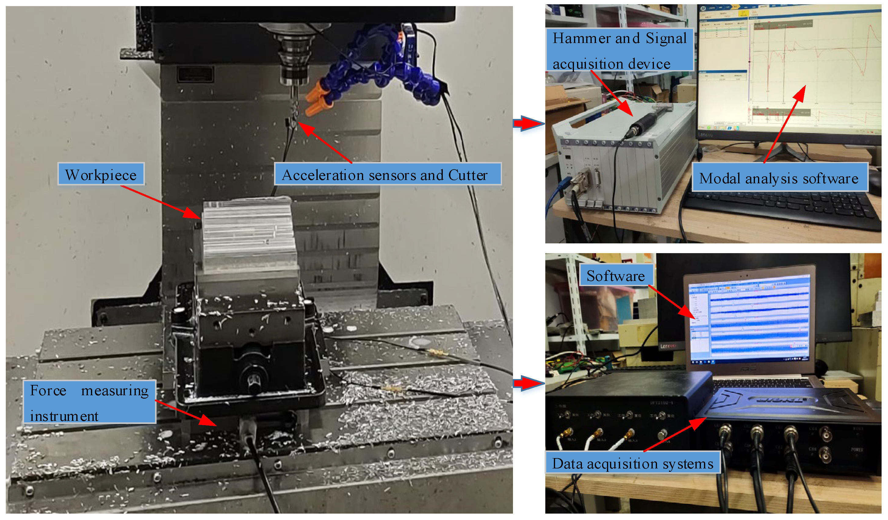
5. Experimental Verification and Analysis

The accuracy of the proposed HFDM needs to be verified by machining experiments. A mode experiment, cutting force coefficient experiment and confirmatory experiment were carried out on the machine tool. The experiment selected a three-tooth end mill with a diameter of 12 mm and a helix angle of 55°. The processed material was 6061 aluminum alloy. The milling experiment system is shown in Figure 3.

In the mode experiment, an impact hammer (Donghua LC02) was used to strike the tool to generate vibration, which was then detected by an acceleration sensor (1A803E) pasted in the X and Y directions at the end of the tool. The modal parameters calculated by a signal acquisition device (Donghua DH 5922) and modal analysis software were shown as follows: ${\omega }_n=1215\times 2\pi$ rad/s, ${\zeta }_x={\zeta }_y=0.039$, $m_t=0.165$ kg and $K_x=K_y=9.596\times {10}^6$ N/m. Through the cutting force coefficient identification experiment, the average cutting forces of nine groups of experiments under different axial cutting depths $a_p$ and different feeds per tooth $f_t$ were measured, as shown in

Table 8. Experiment parameters.

No	${\mathit{f}}_{\mathit{t}}$ (mm)	$\mathit{\Omega }$ (r/min)	${\mathit{a}}_{\mathit{p}}$ (mm)
1	0.05	2000	0.5
2	0.1	2000	0.5
3	0.15	2000	0.5
4	0.05	2000	1
5	0.1	2000	1
6	0.15	2000	1
7	0.05	2000	1.5
8	0.1	2000	1.5
9	0.15	2000	1.5

. The force measuring instrument and uT3408M data acquisition system were used to measure average milling force. Based on the average cutting force model, the radial and tangential cutting force coefficients were calculated by the linear regression method as $K_n=447.33 {\mathrm{N}/\mathrm{m}}^2$ and $K_t=1227.67 {\mathrm{N}/\mathrm{m}}^2$.

Depending on the corresponding parameters obtained from the above experiments, the SLD was calculated by the proposed HFDM, as seen in Figure 4, where $k_{aD}$ = 0.5 and m = 40. In the SLD, six groups of cutting parameters, i.e., A (2840 r/min, 0.8 mm), B (2840 r/min, 1.5 mm), C (4000 r/min, 1.5 mm), D (4500 r/min, 0.8 mm), E (4500 r/min, 1.5 mm) and F (5500 r/min, 1.8 mm), were selected for cutting experimental verification. Three points were in the stable area and three points were in the unstable area. The time-domain diagram and frequency spectrum of the cutting force obtained from the cutting experiment at six points are shown in

Table 9. The results from cutting confirmatory experiments.

Group No.	Time Domain	Frequency Domain
A (stable)
B (chatter)
C (stable)
D (stable)
E (chatter)
F (chatter)

. Compared with points B, E and F, the cutting force signals at points A, C and D were more regular and more stable. The spectral amplitudes of points B, E, and F expand sharply near the natural frequency; the cutting process of these three points is unstable and chatter occurs. The experimental results verified the validity and accuracy of the theoretical prediction by the proposed HFDM.

6. Conclusions

Chatter adversely affects a milling process. Therefore, accurate and efficient stability prediction is very helpful in enhancing machining quality and efficiency. Using multiple interpolation polynomials and precise integration, an HFDM method was developed for the generation of SLDs. In the proposed HFDM, the cubic Newton interpolation polynomial, cubic Hermite interpolation polynomial and linear interpolation were applied to approximate the state term, delay term and periodic coefficient matrix, respectively. Moreover, the PI algorithm was used to calculate the matrix index to improve calculation efficiency and accuracy. The results of the numerical simulation indicated that the proposed HFDM can effectively generate SLDs. The comparison results show that the proposed HFDM can obtain better prediction accuracy and computation efficiency. A milling experiment was also carried out to demonstrate the feasibility of the proposed HFDM. This study is very useful for machining practitioners seeking accurate and efficient methods for stability prediction in milling operations where chatter produces poor quality and productivity and even would hurt the milling machine tool and parts.

According to the SLD provided by the proposed HFDM, field practitioners can select the stable machining parameters within the stable region and hence avoid milling chatter. In addition, since the SLD is frequently associated with the optimization of machining parameters, the SLD information can thus be utilized for selecting the optimal machining parameters to reduce machining time and cost, which further increases the economic advantages.

To perform a complete stability analysis, the proposed HFDM only requires a personal desktop computer with 2.5 GHz i7-11700 CPU and 16 GB memory at about 35 s. This wonderful characteristic enables the proposed HFDM to be applied to stability prediction in real-world applications. Other advantages of the proposed HFDM are that it is relatively easy to implement and that even ordinary practitioners who lack much expertise and experience in machining dynamics can also implement it readily to predict stability in milling operations, provided that appropriate process knowledge is available.

7. Limitations and Recommendations for Future Research

The proposed HFDM can not only accurately but also efficiently predict stability in milling operations, but not without weak points. The proposed HFDM did not consider nonlinear factors, such as the flexibility of the materials and cutter, thermoplastic deformation in the cutting and the run out. Hence, for applying the proposed HFDM in practical machining applications, nonlinear factors should also be included in the formulation of a machining dynamics model to overcome the usage limitation of the proposed method.

In our future research, it will be interesting to expand the proposed HFDM to predict the stability for other machining operations, such as turning and drilling. It will also be interesting to use the SLD information as a constraint condition to optimize the machining parameters to avoid chatter and boost machining productivity.

References

1. Quintana, G.; Ciurana, J. Chatter in machining processes: A review. Int. J. Mach. Tools Manuf. 2011, 51, 363–376. [Google Scholar] [CrossRef]
2. Yue, C.X.; Gao, H.N.; Liu, X.L.; Liang, S.Y.; Wang, L.H. A review of chatter vibration research in milling. Chin. J. Aeronaut. 2019, 32, 215–242. [Google Scholar] [CrossRef]
3. Jung, H.; Hayasaka, T.; Shamoto, E. Mechanism and suppression of frictional chatter in high-efficiency elliptical vibration cutting. CIRP Ann. Manuf. Technol. 2016, 65, 369–372. [Google Scholar] [CrossRef]
4. Zhu, L.; Liu, C. Recent progress of chatter prediction, detection and suppression in milling. Mech. Syst. Signal Process. 2020, 143, 106840. [Google Scholar] [CrossRef]
5. Insperger, T.; Stépán, G. Semi-discretization method for delayed systems. Int. J. Numer. Methods Eng. 2002, 55, 503–518. [Google Scholar] [CrossRef]
6. Altintaş, Y.; Budak, E. Analytical Prediction of Stability Lobes in Milling. CIRP Ann. Manuf. Technol. 1995, 44, 357–362. [Google Scholar] [CrossRef]
7. Jin, G.; Zhang, Q.; Qi, H.; Yan, B. A frequency-domain solution for efficient stability prediction of variable helix cutters milling. Proc. Inst. Mech. Eng. Part C J. Mech. Eng. Sci. 2014, 228, 2702–2710. [Google Scholar] [CrossRef]
8. Merdol, S.D.; Altintas, Y. Multi Frequency Solution of Chatter Stability for Low Immersion Milling. J. Manuf. Sci. Eng. 2004, 126, 459–466. [Google Scholar] [CrossRef]
9. Chen, Z.; Li, Z.; Niu, J.; Zhu, L. Chatter detection in milling processes using frequency-domain Rényi entropy. Int. J. Adv. Manuf. Technol. 2020, 106, 877–890. [Google Scholar] [CrossRef]
10. Liu, C.; Xu, W.W.; Gao, L. Identification of milling chatter based on a novel frequencydomain search algorithm. Int. J. Adv. Manuf. Technol. 2020, 109, 2393–2407. [Google Scholar]
11. Bayly, P.V.; Halley, J.E.; Mann, B.P.; Davies, M.A. Stability of Interrupted Cutting by Temporal Finite Element Analysis. J. Manuf. Sci. Eng. 2003, 125, 220–225. [Google Scholar] [CrossRef]
12. Insperger, T.; Stépán, G. Updated semi-discretization method for periodic delay-differential equations with discrete delay. Int. J. Numer. Methods Eng. 2004, 61, 117–141. [Google Scholar] [CrossRef]
13. Insperger, T.; Stépán, G.; Turi, J. On the higher-order semi-discretizations for periodic delayed systems. J. Sound Vib. 2008, 313, 334–341. [Google Scholar] [CrossRef]
14. Long, X.H.; Balachandran, B. Stability of Up-milling and Down-milling Operations with Variable Spindle Speed. J. Vib. Control. 2010, 16, 1151–1168. [Google Scholar] [CrossRef]
15. Ding, Y.; Niu, J.; Zhu, L.; Ding, H. Numerical Integration Method for Stability Analysis of Milling with Variable Spindle Speeds. J. Vib. Acoust. 2015, 138, 011010. [Google Scholar] [CrossRef]
16. Jiang, S.; Sun, Y.W.; Yuan, X.; Liu, W.R. A second-order semi-discretization method for the efficient and accurate stability prediction of milling process. Int. J. Adv. Manuf. Technol. 2017, 92, 583–595. [Google Scholar] [CrossRef]
17. Yan, Z.; Zhang, C.; Jia, J.; Ma, B.; Jiang, X.; Wang, D.; Zhu, T. High-order semi-discretization methods for stability analysis in milling based on precise integration. Precis. Eng. 2022, 73, 71–92. [Google Scholar] [CrossRef]
18. Sims, N.D.; Mann, B.; Huyanan, S. Analytical prediction of chatter stability for variable pitch and variable helix milling tools. J. Sound Vib. 2008, 317, 664–686. [Google Scholar] [CrossRef] [Green Version]
19. Wan, M.; Zhang, W.-H.; Dang, J.-W.; Yang, Y. A unified stability prediction method for milling process with multiple delays. Int. J. Mach. Tools Manuf. 2010, 50, 29–41. [Google Scholar] [CrossRef]
20. Soriano, C.; Minetaka, H.; Ozaki, N.; Hirogaki, T.; Aoyama, E. Investigation of semi-discretization method in end-milling systems for chatter vibration analysis. Proc. Mech. Eng. Congr. Jpn. 2020, 2020, S13309. [Google Scholar] [CrossRef]
21. Xiong, B.; Wei, Y.; Gu, D.; Zhao, D.; Wang, B.; Liu, S. Chatter stability analysis of variable speed milling with helix angled cutters. Proc. Inst. Mech. Eng. Part B J. Eng. Manuf. 2021, 235, 850–861. [Google Scholar] [CrossRef]
22. Ding, Y.; Zhu, L.; Zhang, X.; Ding, H. A full-discretization method for prediction of milling stability. Int. J. Mach. Tools Manuf. 2010, 50, 502–509. [Google Scholar] [CrossRef]
23. Ji, Y.J.; Wang, X.B.; Liu, Z.B.; Yan, Z.H. An updated full-discretization milling stability prediction method based on the high-er-order Hermite-Newton interpolation polynomial. Int. J. Adv. Manuf. Technol. 2018, 95, 2227–2242. [Google Scholar] [CrossRef]
24. Ji, Y.J.; Wang, X.B.; Liu, Z.B.; Wang, H.J.; Jiao, L.; Zhang, L.; Huang, T. Milling stability prediction with simultaneously considering the multiple factors coupling effects-regenerative effect, mode coupling, and process damping. Int. J. Adv. Manuf. Technol. 2018, 97, 2509–2527. [Google Scholar] [CrossRef]
25. Ding, Y.; Zhu, L.; Zhang, X.; Ding, H. Second-order full-discretization method for milling stability prediction. Int. J. Mach. Tools Manuf. 2010, 50, 926–932. [Google Scholar] [CrossRef]
26. Quo, Q.; Sun, Y.; Jiang, Y. On the accurate calculation of milling stability limits using third-order full-discretization method. Int. J. Mach. Tools Manuf. 2012, 62, 61–66. [Google Scholar] [CrossRef]
27. Zhou, K.; Zhang, J.; Xu, C.; Feng, P.; Wu, Z. Effects of helix angle and multi-mode on the milling stability prediction using full-discretization method. Precis. Eng. 2018, 54, 39–50. [Google Scholar] [CrossRef]
28. Zhang, Y.; Liu, K.; Zhao, W.; Zhang, W.; Dai, F. Stability Analysis for Milling Process with Variable Pitch and Variable Helix Tools by High-Order Full-Discretization Methods. Math. Probl. Eng. 2020, 2020, 1–14. [Google Scholar] [CrossRef]
29. Ding, Y.; Zhu, L.; Zhang, X.; Ding, H. Numerical Integration Method for Prediction of Milling Stability. J. Manuf. Sci. Eng. 2011, 133, 031005. [Google Scholar] [CrossRef]
30. Zhang, Z.; Li, H.G.; Meng, G.; Liu, C. A novel approach for the predictionof the milling stability based on the Simpson method. Int. J. Mach. Tools Manuf. 2015, 99, 43–47. [Google Scholar] [CrossRef]
31. Ozoegwu, C.G. High order vector numerical integration schemes applied in state space milling stability analysis. J. Appl. Math. Comput. 2016, 273, 1025–1040. [Google Scholar] [CrossRef]
32. Zhang, X.J.; Xiong, C.H.; Ding, Y.; Ding, H. Prediction of chatter stability in high speed milling using the numerical differentiation method. Int. J. Adv. Manuf. Technol. 2017, 89, 2535–2544. [Google Scholar] [CrossRef]
33. Dong, X.F.; Qiu, Z.Z. Stability analysis in milling process based on updated numerical integration method. Mech. Syst. Signal Process. 2019, 137, 106435. [Google Scholar] [CrossRef]
34. Tang, X.; Peng, F.; Yan, R.; Gong, Y.; Li, Y.; Jiang, L. Accurate and efficient prediction of milling stability with updated full-discretization method. Int. J. Adv. Manuf. Technol. 2016, 88, 2357–2368. [Google Scholar] [CrossRef]
35. Yan, Z.; Wang, X.; Liu, Z.; Wang, D.; Jiao, L.; Ji, Y. Third-order updated full-discretization method for milling stability prediction. Int. J. Adv. Manuf. Technol. 2017, 92, 2299–2309. [Google Scholar] [CrossRef]
36. Huang, C.; Yang, W.A.; Cai, X.L.; Liu, W.C.; You, Y.P. An efficient third-order full-discretization method for prediction of re-generative chatter stability in milling. Shock Vib. 2020, 2020, 1–16. [Google Scholar]
37. Yan, Z.; Zhang, C.; Jiang, X.; Ma, B. Chatter stability analysis for milling with single-delay and multi-delay using com-bined high-order full-discretization method. Int. J. Adv. Manuf. Technol. 2020, 111, 1401–1413. [Google Scholar] [CrossRef]
38. Dai, Y.; Li, H.; Yang, G.; Peng, D. A novel method with Newton polynomial-Chebyshev nodes for milling stability prediction. Int. J. Adv. Manuf. Technol. 2021, 112, 1373–1387. [Google Scholar] [CrossRef]
39. Dai, Y.; Li, H.; Peng, D.; Fan, Z.; Yang, G. A novel scheme with high accuracy and high efficiency for surface location error prediction. Int. J. Adv. Manuf. Technol. 2021, 118, 1317–1333. [Google Scholar] [CrossRef]
40. Ding, Y.; Zhu, L.M.; Zhang, X.J.; Ding, H. On a numerical method for simultaneous prediction of stability and surface loca-tion error in low radial immersion milling. J. Dyn. Syst. Meas Control Trans. ASME 2011, 133, 024503. [Google Scholar] [CrossRef]
41. Dai, Y.B.; Li, H.K.; Xing, X.Y.; Hao, B.T. Prediction of chatter stability for milling process using precise integration method. Precis Eng. J. Int. Soc. Precis Eng. Nanotechnol. 2018, 52, 152–157. [Google Scholar] [CrossRef]
42. Dai, Y.; Li, H.; Wei, Z.; Zhang, H. Chatter stability prediction for five-axis ball end milling with precise integration method. J. Manuf. Process. 2018, 32, 20–31. [Google Scholar] [CrossRef]
43. Li, H.K.; Dai, Y.B.; Fan, Z.F. Improved precise integration method for chatter stability prediction of two-DOF milling system. Int. J. Adv. Manuf. Technol. 2018, 101, 1235–1246. [Google Scholar] [CrossRef]
44. Yang, W.-A.; Huang, C.; Cai, X.; You, Y. Effective and fast prediction of milling stability using a precise integration-based third-order full-discretization method. Int. J. Adv. Manuf. Technol. 2020, 106, 4477–4498. [Google Scholar] [CrossRef]
45. Farkas, M. Periodic Motions; Springer: Berlin, Germany, 1994. [Google Scholar]
Figure 1. Unfold chart of the milling process.
Mathematics 11 02629 g001
Figure 2. The flowchart of the proposed HFDM for stability prediction in milling operations.
Mathematics 11 02629 g002
Figure 3. Experimental set-up for milling experiment.
Mathematics 11 02629 g003
Figure 4. The SLD results of the proposed HFDM.
Mathematics 11 02629 g004