Article

Multi-Objective Optimization for Controlling the Dynamics of the Diabetic Population

1
Engineering Science Laboratory, FPT, Sidi Mohamed Ben Abdellah University, Fez 30000, Morocco
2
Centre for Computational Science and Mathematical Modelling, Coventry University, Priory Road, Coventry CV1 5FB, UK
3
Department of Robotics and Production System, University Politehnica of Bucharest, 020771 Bucharest, Romania
4
MorphoSciences Research Laboratory, Faculty of Medicine and Pharmacy, Cadi Ayyad University, Marrakech 40001, Morocco
5
Biosciences and Health Laboratory, Faculty of Medicine and Pharmacy, Cadi Ayyad University, Marrakech 40001, Morocco
*
Authors to whom correspondence should be addressed.
Mathematics 2023, 11(13), 2957; https://doi.org/10.3390/math11132957
Submission received: 23 May 2023 / Revised: 26 June 2023 / Accepted: 29 June 2023 / Published: 2 July 2023
(This article belongs to the Special Issue Dynamic Modeling and Simulation for Control Systems, 2nd Edition)

Abstract

:
To limit the adverse effects of diabetes, a personalized and long-term management strategy that includes appropriate medication, exercise and diet has become of paramount importance and necessity. Compartment-based mathematical control models for diabetes usually result in objective functions whose terms are conflicting, preventing the use of single-objective-based models for obtaining appropriate personalized strategies. Taking into account the conflicting aspects when controlling the diabetic population dynamics, this paper introduces a multi-objective approach consisting of four steps: (a) modeling the problem of controlling the diabetic population dynamics using a multi-objective mathematical model, (b) discretizing the model using the trapezoidal rule and the Euler–Cauchy method, (c) using swarm-intelligence-based optimizers to solve the model and (d) structuring the set of controls using soft clustering methods, known for their flexibility. In contrast to single-objective approaches, experimental results show that the multi-objective approach obtains appropriate personalized controls, where the control associated with the compartment of diabetics without complications is totally different from that associated with the compartment of diabetics with complications. Moreover, these controls enable a significant reduction in the number of diabetics with and without complications, and the multi-objective strategy saves up to 4% of the resources needed for the control of diabetes without complications and up to 18% of resources for the control of diabetes with complications.

1. Introduction

Diabetes is a permanent disease resulting from the pancreas’ incapacity to generate insulin, or the body being incapable of utilizing the insulin properly. According to forecasts by the International Diabetes Federation (IDF), by 2045, one person in eight, or approximately 783 million individuals, will be suffering from diabetes, representing an average increase of 46% [1]. More than 90% of people living with diabetes are type 2 diabetics. Urbanization, an aging population, reduced physical activity and the increased prevalence of overweight and obesity are the major contributors to the increase in type 2 diabetes. According to the IDF’s 2021 report, diabetes accounted for at least USD 966 billion in healthcare costs (9% of the total adult budget). Diabetes can lead to serious complications, among them vision loss, cardiovascular problems, kidney insufficiency, cerebrovascular accidents, nerve damage and lower-limb amputations. The key measures capable of mitigating this damage include appropriate medication, adapted physical exercise [2] and personalized diet [3,4,5]. To determine an optimal control and implement these measures, several mathematical control models have been proposed in the literature. Unfortunately, these models do not distinguish between the different components of the diabetic population we wish to control, while certain conflicting characteristics are implicitly embedded in this problem. This results in standard strategies that are adequate for some patients but not appropriate for others [6,7].
This work proposes a new approach to control the dynamics of the diabetic population based on a multi-objective dynamic model, using multi-objective swarm intelligence optimizers and soft clustering algorithms.
Most of the strategies aimed at controlling the dynamics of the diabetic population are based on single-objective mathematical models, which formulate the optimal control using the Pontryagin’s maximum principle and decompose the model using various numerical techniques to estimate the control [8,9,10,11]. Numerical methods employing Pontryagin’s maximum principle result in controls that are prohibitively resource-hungry in terms of both personnel and material. To overcome this problem, the authors of [2] used several heuristic methods to estimate a control by introducing an adequate objective function that makes a compromise between the components of the model proposed in [8]. However, focusing on a single objective leads to controls that heavily minimize certain compartments at the detriment of others. In addition, this kind of solution provides a unique policy that may not be suitable in some contexts or may not be appropriate.
In this work, we introduce a multi-objective strategy to control the dynamics of a diabetic population, implementing three compartments, i.e., pre-diabetics, diabetics, and diabetics with complications, and consisting of the following steps: (a) the introduction of two controls to protect diabetics from developing complications, (b) the introduction of two objectives functions to reduce the size of the two last compartments and the necessary resources to realize such a reduction, (c) the discretization of the obtained model using the Euler–Cauchy method and the trapezoidal rule, (d) the construction of two appropriate objective functions that make a compromise between the components of the model, and (e) employing NSGA-II [12] and MOFA [13] multi-objective optimization algorithms to build the Pareto front that presents the set of control actions to the customers. In step (c), we evaluated the error due to the discretization process. NSGA-II and MOFA produce a set of controls from which the user has to select the appropriate one considering its requirements. To assist the user, we structured the Pareto solutions front using two soft clustering methods: the Gaussian mixture model (GMM) [2] and Fuzzy-CMeans (FCM) [14]. The employed soft computing methods based on fuzzy or probabilistic approaches provide decision system makers with the necessary capabilities to deal with imprecise and incomplete information. A soft clustering method permits us to have an observation that belongs to two or more clusters. The optimal number of groups was selected on the basis of the silhouette criteria [14]. The experimental results show that the proposed multi-objective approach offers several effective and personalized controls that will enable experts to implement diversified group therapies to alleviate the human and material damage of diabetes.
The main contributions of this paper are summarized as follows:
(1)
A multi-objective mathematical model for controlling the dynamics of the diabetic population is introduced;
(2)
A discretization of the proposed model is realized based on the trapezoidal rule and the Euler–Cauchy method (we demonstrate that this error is bounded);
(3)
Two multi-objective optimizers are used to solve the proposed multi-objective model;
(4)
As a first postprocessing phase, FFT convolution is used to clean the noise from the control;
(5)
As a second post-processing phase, two soft clustering methods are used to structure the Pareto front.
The rest of the paper is organized as follows: Section 2 presents some related works. Section 3 provides a methodology overview. Section 4 presents the proposed multi-objective mathematical model. Section 5 presents the employed computational intelligence algorithms (NSGA-II, MOFA, FCM and GMM). Section 6 discusses the experimental results obtained using our approach. Finally, Section 7 gives some conclusions and future directions.

2. Related Works

Faced with a large population of diabetics, a long-term strategy (group therapy) is needed that involves dividing this population into a reasonable number of compartments, then estimating the magic combinations comprising diet, exercise and medication for each compartment.
To meet these needs, a number of mathematical models have been developed, in particular dynamic models of the diabetic population. Various compartments have been considered, i.e., pre-diabetic people, diabetic people without complications, people with complications, healthy people and other types [15,16,17,18,19]. All the dynamic models of diabetes proposed in the literature focus on a single objective function and follow the same steps, with slight differences depending on the types of diabetic groups studied. At first, research was performed only on two types of compartments, the compartment of people with diabetes and prediabetic people. In 2014, the first controlled population dynamics model of diabetes was put forward [20]. It considered three types of populations: pre-diabetic individuals, diabetic individuals without complications and diabetic individuals with complications [20]. The authors proposed this controlled diabetic population model to reduce the negative effects of this disease and used the Gumel numerical method [21] to solve the system. They also proposed a control strategy over a period of 120 months. Subsequently, another controlled dynamic model of the diabetic population, based on a new control strategy, was proposed in [22]; this time, they thought of dividing the population into two types of compartments, which were the uncomplicated diabetic individuals and the diabetic individuals with complication. Unfortunately, this approach excludes many diabetes-related groups and fails to specify how to control a very large population size with the same control strategy. In 2018, the authors of [23] introduced a population control model for diabetics, implementing five compartments, but the proposed model takes into account people with disabilities, which is not the most prevalent general case. Consequently, this control cannot be generalized.
An alternative study, which has some overlap with our study, examines the fact of being pregnant [24]. Unfortunately, this study focuses only on women, and more specifically on pregnant women. Moreover, the control phase has not yet been carried out. In [25], authors suggested a reduced monitoring framework using the time-discrete method, which models the progression of prediabetes to diabetes with and without complications and the impact of the lifestyle context. Anther work [26], by the same authors, provided a mathematical model of the diabetic population split into six compartments considering other aspects such as the effects of genetics and behavioral factors. The authors of the study suggest that in order to decrease the proportion of diabetics, three controls could be implemented: an awareness program through education and media, therapy and psychological assistance with follow-up. In the end, several strategies were proposed in [25,26], but they lead to confusion for doctors, and the proposed controls are difficult for non-mathematicians to understand. In [8], the authors investigated a model that outlines the evolution of the population, as well as the pain of diabetic subjects with the socio-environmental effect depending on the age category; the authors suggested an optimized monitoring plan to protect patients from the negative influence of a lifestyle that causes them to develop complications. Numerical methods, employing Pontryagin’s principle, result in controls that are prohibitively expensive in terms of human and material resources. Recently, in [2], we used heuristic methods to estimate a control based on a fitness function that achieves a compromise between constraints and the model’s objective function. However, implementing conflicting criteria in a single function results in non-personalized standard controls. This paper introduces a new approach based on a multi-objective model, which we solve with two multi-objective swarm optimizers. In order to help the user select a suitable control from the Pareto front, we also employ two soft clustering methods as mentioned in the previous section.

3. Methodology Overview

Notations
Time variables: we denote by T the control period and by h the time step.
Compartments: E ,   I ,   D and C are the number of pre-diabetics, the incidence of being prediabetic, the number of diabetics and the number of diabetics with complications.
Parameters: In the system described in Equation (1), μ is the biological death ratio, β 1 is the risk of acquiring diabetes mellitus (DM), β 2 is the estimate of the likelihood that an individual with DM will develop a complication, β 3 is the risk of developing complicated DM, γ is the success ratio for complications, ν is the degree to which severely disabled individuals become seriously handicapped and δ is the death ratio caused by medical complications.
Controls: u 1 and u 2 are the functions introduced to control the compartments of diabetics with and without complications.
Model
Variables: we introduced two functions ( u 1 and u 2 ), in model (1), to control the compartments D and C during the period T ; see system (2).
First objective function: this function was introduced to minimize the number of diabetic D and the resources required to realize this objective (i.e., u 1 ).
Second objective function: this function was introduced to minimize the number of diabetics with complications C and the resources required to realize this objective (i.e., u 2 )
Constraints: ordinary differential equation that governs the exchange between different compartments in the presence of the controls.
Discretization
Objective functions: The first and the second objective functions implement integral operators to consider the number of diabetics with and without complications and the resources required to control these compartments during the period T . To transform these integral to a discrete sum, we used the trapezoidal rule based on time step h .
Constraints: to transform the differential equations of the proposed model into a combinatorial system, we used the Euler–Cauchy method because of its simplicity.
Error estimation: in lemma 1 and proposition 1, we demonstrate that the error due to the discretization is still bounded with a cubic function that implements all the outputs of the multi-objective model.
Smart local search
To estimate the controls u 1 and u 2 , we used two multi-objective local search methods, namely the NSGA [12,27] and MOFA [13] algorithms; the configurations of these methods were experimentally chosen. Here [ T / h ] + 1 represents the integer par of T / h .
Post-processing
Features extraction: to avoid high-dimensional vectors ([T/h]), when structuring the control space, we extracted the relevant information by adopting certain criteria (control fluctuation, control cost, quality of compartments and spatial characteristics).
Structuring of the Pareto front: NSGA-II and MOFA produce a set of controls that are difficult to exploit, so we used two soft clustering methods, GMM [14] and FCM [28], to summarize the Pareto front.
Fluctuation corrections: To correct fluctuations caused by successive approximations, we used the FFT convolution operator and test several masks of different sizes ( 4 × 4 ,   . . . , 10 × 10 ). In this sense, given a function, represented by the matrix U, whose fluctuations we want to eliminate, we chose a suitable kernel function K, represented by a matrix of ones modified by a suitable weight w , and the convolution formula is given by j , k   C i , j = p , q U ( p , q ) K ( j p + 1 , k q + 1 ) .
The size of the kernel K and w were experimentally chosen.
Performance evaluation
The control quality was measured using three criteria: (a) the rate of growth of E : the faster it is, the better the control; (b) the rate of decay of D and C : the faster the decay, the better the control; and (c) the values taken by u 1 and u 2 : the smaller they are, the better the control.

4. Multi-Objective Diabetic Control Model

4.1. Single-Goal Control Model

Let E ( t ) , D ( t ) and C ( t ) be the compartment of pre-diabetic individuals, the compartment of diabetic individuals without complication and the compartment of diabetic individuals with complication, respectively. Derouich et al. [20] introduced the following mathematical model:
d E ( t ) d t = I ( μ + ( β 3 + β 1 ) ( 1 u ( t ) ) ) E ( t ) d D ( t ) d t = β 1 ( 1 u ( t ) ) E ( t ) ( μ + β 2 ( 1 u ( t ) ) ) D ( t ) + γ C ( t ) d C t d t = β 3 1 u t E t + β 2 1 u t D t μ + γ + ν + δ C t
u represents the intervention of the endocrinologist [medication potency level (1 mg, …, 10 mg), diet level (the glycemic load not to be exceeded), type of exercise (the number of minutes of walking, type of running...)], I is the effect of the presence of pre-DM, μ is the biological death ratio, β 1 is the risk of acquiring DM, β 2 is the estimate of the likelihood that an individual with DM will develop a complication, β 3 is the risk of developing complicated DM, γ is the success ratio for complications, ν is the degree to which severely disabled individuals become seriously handicapped and δ is the death ratio caused by medical complications.
The function they sought to minimize in [20] is of the following form:
Γ ( u ) = 0 T ( D ( t ) + C ( t ) + K u 2 ( t ) ) d t
K R + and all the feasible controls of one goal model form a set denoted U . u is said to be feasible if it is measurable and the system (1) has at least one solution. A feasible control is expressed in percent, i.e., 0 u t 1 , t 0 ,   T .
Problems:
For a given decision u , the 0 T D t + C t + K u 2 ( t ) d t and 0 T D t d t can be minimal and 0 T C t d t is very large, as the terms in Γ are in conflict with each other.
In practice, it is difficult to set up a tradeoff between D , C and u via a penalty constant. In fact, to evacuate compartment D, there are three possibilities: move patients from D to E or move patients from D to C, or both. To evacuate compartment C, there is only one possibility: move patients from C to D. So, the two compartments D and C are in conflict. A possible scenario: if the number of diabetic patients with complications is very small, compared to D, a wrong choice of aggregation parameters can give wrong information to the optimization methods and the number of patients with complications can receive elements from D while the objective function is minimal (for a given local solution). When dealing with conflicting cost functions, a single solution is not reasonable because a solution that may be appropriate in one context may not be appropriate in another. The characteristics of patients in D are not similar to the ones of C . Therefore, the regulation of the system requires individualized policies that take this difference into account.
The Pontryagin principle implies very complex mathematical formulas; moreover, it leads to an expansive strategy that consumes all existing resources.

4.2. Multi-Objective Control Model

Decision variables: To act on E and D with two separate strategies, we introduced two controls, u 1 to control E and u 2 to control D . u 1 and u 2 are two measurable functions defined on [ 0 ,   T ] and take their values in [ 0 ,   1 ] . Practically speaking, it is impossible to estimate the decision functions at each instant t, and that is why we estimated these functions at d instants t 1 , , t d from [ 0 ,   T ] such that t i + 1 t i = c o n s t a n t = h and T h = d , and let us denote by u 11 , , u 1 d   and   u 21 , , u 2 d the obtained values.
Constraints: By introducing u 1 and u 2 in the system ( 1 ) , we prevented 1 u 1 t % of prediabetic people and 1 u 2 t % of people with diabetes from joining the upper compartments; thus, we obtained the following system:
d E t d t = I μ + β 3 + β 1 1 u 1 t E t d D t d t = β 1 1 u 1 t E t μ + β 2 1 u 2 t D t + γ C t d C t d t = β 3 1 u 1 t E t + β 2 1 u 2 t D t μ + γ + ν + δ C t
We discretized the system ( 2 ) using the time step h defined before, and we obtained the following system:
E i + 1 = I h μ + β 3 + β 1 1 u 1 , i h E i + E i D i + 1 = β 1 1 u 1 , i h E i μ + β 2 1 u 2 , i h D i + γ h C i + D i C i + 1 = β 3 1 u 1 , i h E i + β 2 1 u 2 , i h D i μ + γ + ν + δ h C i + C i i = 0 , , d 1
where u ~ p = ( u p , 0 , , u p , d ) , p = 1,2 .
Objective functions: We introduced the following two objective functions:
Γ 1 ( u 1 , u 2 ) = 0 T C t + K u 1 2 t d t   a n d   Γ 2 ( u 1 , u 2 ) = 0 T D t + K u 2 2 t d t
We used the trapezoidal rule to estimate Γ 1 and Γ 2 and then obtained the following objective functions:
Γ 1 u 1 , u 2 Γ ~ 1 ( u ~ 1 , u ~ 2 ) = h 2 i = 0 d 1 C i + 1 + C i + K h 2 i = 0 d 1 ( u 1 , i + 1 2 + u 1 , i 2 )
Γ 2 u 1 , u 2 Γ ~ 2 [ u ~ 1 , u ~ 2 ] = h 2 i = 0 d 1 D i + 1 + D i + K h 2 i = 0 d 1 ( u 2 , i + 1 2 + u 2 , i 2 )
We denote by U 1,2 the set of the pair feasible control.
The multi-objective problem we propose in this work is given by:
M i n   Γ ~ 1 [ u ~ 1 , u ~ 2 ]               M i n   Γ ~ 2 [ u ~ 1 , u ~ 2 ] S u b j e c t   t o [ u ~ 1 , u ~ 2 ] [ 0 ,   1 ] 2 d E ~ , D ~ , C ~     s o l u t i o n   o f   ( 3 )
Convexity of the problem (4): We have i = 0 , , d 1 and j = 1 ,   2 ; the function [ u ~ 1 , u ~ 2 ] u j , i + 1 2 + u j , i 2 is convex.
Then j = 1 ,   2 , and the function [ u ~ 1 , u ~ 2 ] i = 0 d 1 ( u j , i + 1 2 + u j , i 2 ) is convex;
As  K h 2 > 0 , then j = 1 ,   2 ; the function [ u ~ 1 , u ~ 2 ] Γ ~ j [ u ~ 1 , u ~ 2 ] is convex.
We have i = 0 , , d 1 , the function
F ( u ~ 1 , u ~ 2 ) = I h μ + β 3 + β 1 1 u 1 , i h E i + E i E i + 1 β 1 1 u 1 , i h E i μ + β 2 1 u 2 , i h D i + γ h C i + D i D i + 1 β 3 1 u 1 , i h E i + β 2 1 u 2 , i h D i μ + γ + ν + δ h C i + C i C i + 1
is linear; thus, F is convex.
Finally, the problem (4) is convex.
As we have shown that the problem (4) is convex, we used gradient methods to solve it:
(a)
The primary methods used were gradient descent algorithms [29];
(b)
Dual methods, which exploit convexity to calculate the gradient of the dual max–min, were also used [30];
(c)
The substitution and the decomposition Lagrange methods that introduce a copy variable to decompose the initial problem to two sub-problems [31]: the first one does not have any constraints (for which we can use gradient descent, among others) and the second one does not have objective functions (for which we can use back tracking methods, among others).
In this sense, we have to transform the multi-objective functions to a single-objective function using aggregation weights; as a result, we find ourselves in front of a system of 3 d constraints plus 2 d positivity constraints. In this work, we preferred to use heuristic methods that only meet the 0 u ~ j , i 1   i = 0 , , d 1   a n d   j = 1 ,   2 positivity constraints, i.e., 2 d , which are easily introduced in Matlab’s “gamultiobj” as bounds. To avoid the 3 d constraints, given an estimation of the control, at the iteration k, we used an interpolation method (for example the spline method) to transform the discrete control u ~ to the continuous control u; then, we called for the Euler–Cauchy method to approximate the compartments C and D ; after that, we estimated the value of the function Γ ~ j ( u ~ 1 , u ~ 2   ( j = 1 ,   2 ) .
Error of approximation: In this section, we estimate the error related to the approximation of the integral using the trapezoidal rule. We introduced the following functions:
f 1 t = C + K u 1 2 and f 2 t = D + K u 2 2
i { 1 ,   2 } , we set M i = max t [ 0 ,   T ] | u i ( t ) | and M i = max t [ 0 ,   T ] | u i ( t ) |
Lemma 1.
Considering the system (2), we have:
f 1 α M 1 + α M 2 + 31 α 2 + α P + 2 K M 1 + 2 K M 1 2
f 2 α M 1 + α M 2 + 17 α 2 + α P + 2 K M 2 + 2 K M 2 2
where  P  is the size of the population and  α = m a x { μ , γ , ν , δ , β 1 , β 2 , β 3 } .
Proof of Lemma 1.
 
We have f 1 = C + 2 K u 1 u 1
Thus f 1 = β 3 1 u 1 E + β 2 1 u 2 D μ + γ + ν + δ C + 2 K u 1 u 1
Then f 1 t = β 3 u 1 E + β 3 1 u 1 E β 2 u 2 D + β 2 1 u 2 D μ + γ + ν + δ C + 2 K u 1 u 1 + 2 K ( u 1 ) 2
Thus f 1 = β 3 u 1 E + β 3 1 u 1 I μ + β 3 + β 1 1 u 1 E β 2 u 2 D + β 2 1 u 2 β 1 1 u 1 E μ + β 2 1 u 2 D + γ C μ + γ + ν + δ β 3 1 u 1 E + β 2 1 u 2 D t μ + γ + ν + δ C + 2 K u 1 u 1 + 2 K u 1 2
Then f 1 = β 3 u 1 β 3 1 u 1 μ + β 3 + β 1 1 u 1 + β 2 β 1 1 u 1 1 u 2 μ + γ + ν + δ β 3 1 u 1 E + β 2 u 2 β 2 1 u 2 μ + β 2 1 u 2 μ + γ + ν + δ β 2 1 u 2 D + β 2 1 u 2 γ + μ + γ + ν + δ 2 C + 2 K u 1 u 1 + 2 K u 1 2 + β 3 1 u 1 I
Thus f 1 α M 1 + α M 2 + 31 α 2 + α P + 2 K M 1 + 2 K M 1 2
Following the same steps, we find f 2 α M 1 + α M 2 + 17 α 2 + α P + 2 K M 2 + 2 K M 2 2 . □
Proposition 1.
Let  u 1 , u 2  be the optimal control of the problem (P). The error associated with the trapezoidal rule discretization is bounded by the number
E = T h 2 12 [ ( α M 1 + α M 2 + 31 α 2 + α ) P + 2 K M + M 2 ]
where  M = max   M 1 , M 2 , M 1 , M 2 .
Proof of the Proposition 1.
Consider the integral I n t e g = a b f ( t ) d t ; Rahman Qzi et al. showed that the error of the trapezoidal rule is estimated by [32]:
E r r o r = b a 3 12 N 2 f ( ξ )
where N is the number of the used points in a , b .
In our case, a = 0   a n d   b = T ,   a n d   N = d = T / h (h is the step of the discretization).
However, we demonstrated before, in Lemma 1, that
f 1 α M 1 + α M 2 + 31 α 2 + α P + 2 K M 1 + 2 K M 1 2   and   f 2 α M 1 + α M 2 + 17 α 2 + α P + 2 K M 2 + 2 K M 2 2
Thus f i α M 1 + α M 2 + 31 α 2 + α P + 2 K M 1 + 2 K M 1 2
Thus, the discretization error is given by
E = T 3 12 N 2 f i ( ξ ) T h 2 12 [ ( α M 1 + α M 2 + 31 α 2 + α ) P + 2 K M + M 2 ]
The reason why our approach is of practical rather than conceptual importance is that it offers more freedom to fragment the control: the first is focused on E and the second is about D . We will not elaborate too much in the proofs of the results relating to the invariance and the existence of the solution of the proposed multi-objective model for every pair of controls ( u 1 , u 2 ) .
Invariance: based on the Gronwall inequality (applied to the model ( 2 ) ) [15], we demonstrate that E ( t ) > 0 , D ( t ) > 0 , C ( t ) > 0 , and N t = E t + D t + C t I / μ .
Existence: By adopting the same procedures as in [15], we proved that the right-hand members of the Equation (2) are Lipschitzian. The difference between the proofs given in [15] were the considered bounds. In our situation, these bounds implemented the controls u 1 and u 2 , and since ( u 1 , u 2 ) U 1 × U 2 , these results are always true. □
Theorem 1.
Let us consider the next problem:
M i n   Γ 1 u 1 , u 2                 M i n   Γ 2 u 1 , u 2 S u b j e c t   t o ( u 1 , u 2 ) U 1 × U 2 E , D , C     s o l u t i o n   o f   ( 2 )
A Pareto front of non-dominant optimal decisions exists (called the Pareto optimal control).
Proof of the Theorem 1:
Without going into details, the existence of an optimal front can be proved by applying the finding of Fleming and Rishel [33] and by following the steps mentioned below:
Γ 1 u 1 , u 2 = 0 T C t + K u 1 2 t d t   a n d   Γ 2 ( u 1 , u 2 ) = 0 T D t + K u 2 2 t d t are convex in ( u 1 , u 2 ) ;
U 1 × U 2 is convex.
The right-hand sides of the system Equation ( 2 ) are continous, bounded and can be written as a linear function of u 1   a n d   u 2 with coefficients depending on time and state;
The integral of the objective functionals, C ( t ) + K u 1 2 ( t ) and D ( t ) + K u 2 2 ( t ) , are clearly convex on U 1 × U 2 ;
We have C t + K u 1 2 t α 1,1 + α 1,2 u 1 2 and D t + K u 2 2 t α 2,1 + α 2,2 u 2 2 where α 1,1 = inf t [ 0 ,   T ] D ( t ) and α 2,1 = inf t [ 0 ,   T ] C ( t ) and α 1,2 = α 2,2 = K . □

4.3. Pareto Controls Characterization

The Pareto curve is formed by non-dominated controls (we denote by m the size of the pareto set). We estimated these controls on several points, say d , of the control interval [ 0 ,   10 ] years; generally, d is very large compared to m , which affects the quality of the grouping. In this part, we extracted the most important features that describe the controls basing on four criterions: the controls fluctuation, the cost of the controls, the spatial characteristics of the decisions and the quality of the controls.
Fluctuation characteristics: First, we removed the linear trend from the controls u 1 and u 2 using FFT processing [34], and we obtained the corrected controls u 1 and u 2 . Two fluctuation features were extracted in this phase: n o r m ( u 1 u 1 ) and n o r m ( u 2 u 2 ) .
Control cost: The total resources mobilized to control the compartments D and C ; these were estimated by the sum of the controls on the control duration. In this sense, we have: s u m ( u 1 ( t ) / t [ 0 , T ] )   a n d   s u m ( u 2 ( t ) / t [ 0 ,   T ] ) .
Spatial characteristics: the spatial characteristics were measured based on the coefficients of the polynomial interpolation of the controls.
Quality of Compartments: The adequacy of the different compartments was measured by DIST = distance (compartment without control, compartment with control). We obtained three compartment features: d i s t E w , E , d i s t ( D w , D ) and d i s t ( C w , C ) . The greater the DIST, the better the control.

5. Smart Algorithms

5.1. Swarm Intelligence Optimizers

The metaheuristic algorithms were designed based on simulating natural phenomena and laws, which have better global search ability. The most important concept of multi-objective optimization is the Pareto front; it is the curve of the non-dominated points considering the different objective functions at the same time.
Figure 1 illustrates the notion of a Pareto front. Considering the blue line, if we prefer one objective function, then we disadvantage the other objective function.
In this section, we provide the main ideas of two well-known swarm intelligence optimizers that produce local Pareto fronts when solving a multi-objective optimization: NSGA-II and MOFA. As the appropriate crossover of local search methods allows us to overcome the shortcomings of the parent methods, it was possible to use some recent hybrid methods to solve the proposed model, such as the hybrid firefly genetic [3] approach, the cuckoo search-based metaheuristic approach [35] and the hybrid marine predator sine–cosine [36] algorithms.

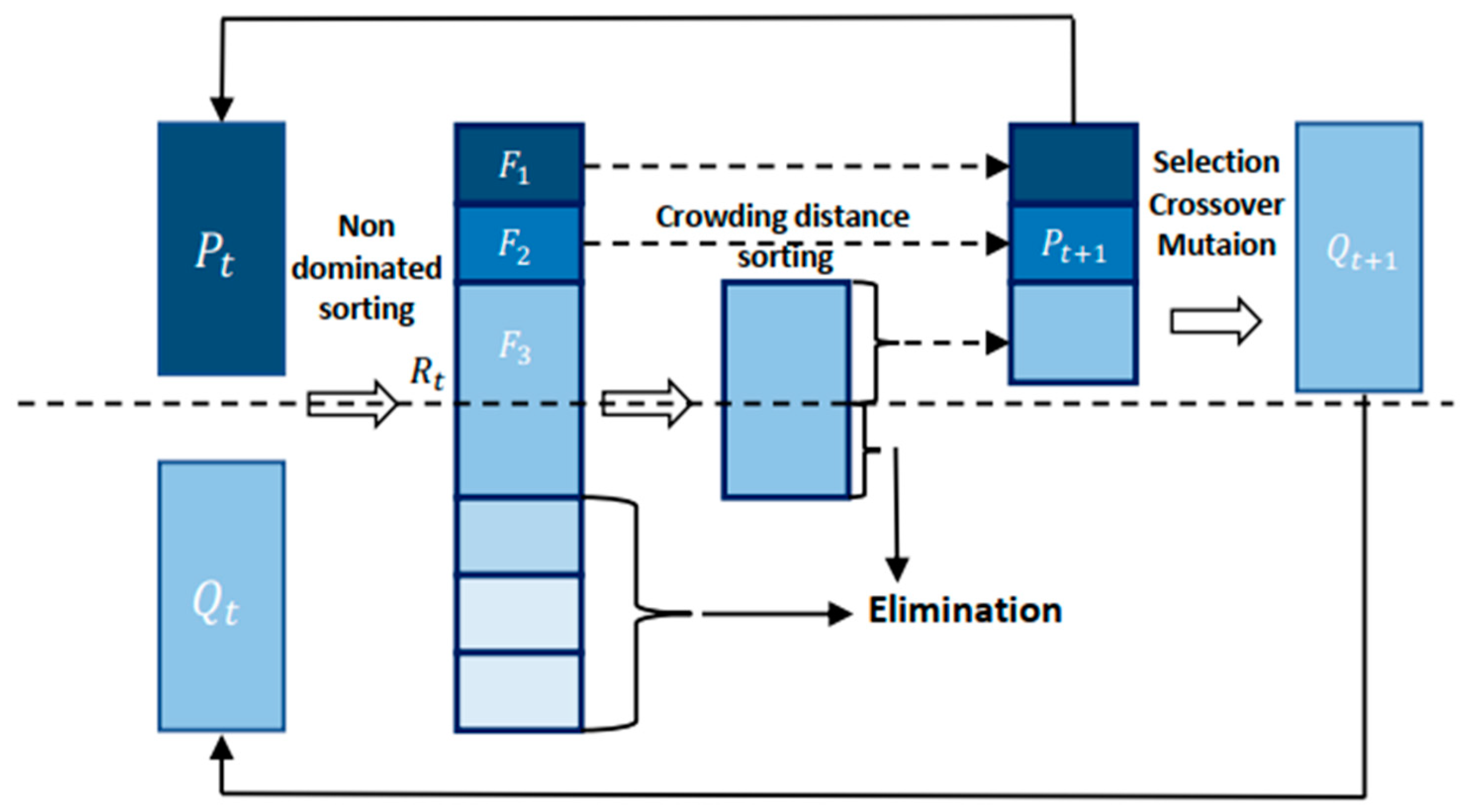
5.1.1. Non-Dominated Sorting Genetic Algorithm II

NSGA-II tends to encourage higher-order chromosomes to appear in the future population [12,27]. The controlled evolutionary selection also encourages the chromosomes to participate in a reasonable diversity of the population in spite of their current weakness. The Pareto fraction limits the number of chromosomes in the solution set. The distance function ensures diversity on the front while promoting chromosomes with an acceptable distance from the front.
The different phases of NSGA-II are shown in Figure 2. The initialization is based on the constraints of the studied problem. Then, the procedure called the non-dominated sorting process about the dominance notion is started. After that, the chromosomes are selected based on two criteria: rank and crowding distance. Then, selection via the tournaments method implementing the crowded-comparison operator is used to select the individuals. The crossover operator and the mutation operator are used to produce chromosomes. The new production is filled by each of the successive borders until the current population size exceeds the tolerated size.
NSGA-II has the advantages of simple coding and excellent performance, and has been successfully applied for solving real-world problems, e.g, solving the flow-shop scheduling problem [37], optimal diet problem [4], data classification [38], Louver configuration [39], 3D laser scanning scheme for engineering structures [40], UAV path planning [41], optimal lane change path planning [42], green pepper detection [43], optimal configuration of landscape storage in public buildings [44], etc.

5.1.2. Multi-Objective Firefly Algorithm

MOFA is inspired by the behavior of fireflies [13]. The basic one-objective version is based on the following rules [27]:
(a)
Fireflies have the ability to attract other fireflies, no matter which sex they are.
(b)
The attraction is positively proportional to the brightness. If all the fireflies have nearly the same degree of brightness, then one or more fireflies are moving.
(c)
The luminosity of a firefly is calculated from the cost function.
If d i j is the distance between two fireflies i and j, then the variability of attractiveness δ i j is estimated by:
δ i j = δ 0 exp σ d i j 2
The parameters δ 0 and σ are chosen by the user.
If x i t and x j t are the present position of the fireflies i and j , respectively, the FA algorithm uses the following equation to calculate the next position of the ith firefly:
x i t + 1 = x i t + δ i j x j t x i t + α t ε i t
α t and ε i t are the global and local random series corresponding to the ith firefly.
An extension of the basic ideas of FA leads to MOFA, presented in Figure 3.
Based on the cost functions and the constraints of the problem to be solved, we defined appropriate objective functions. A swarm of fireflies was uniformly chosen from the research space to ensure the same chances to different regions to be explored. The basic cycle starts by measuring the brightness of all individuals in the swarm, and each pair of elements is measured against each other. Then, a smart pairing is carried out on the base of a convex weight matrix. The non-dominated solutions are then forwarded to the following step. Upon termination of a given number of repetitions, n non-dominated solutions are achieved to approach the correct Pareto front.
In this context, MOFA has the advantages of simple coding and a smaller number of parameters to use and has been successfully applied recently for solving interesting problems, such as an energy-efficiency problem [45], automatic EEG channel selection problem [46], reference point reconstruction problem [47], integrated process planning and scheduling problem [48], stochastic techno-economic–environmental optimization [49], optimization of concentric circular antenna array [50], VLSI Floorplanning problem [51], configuration of power quality control device problem [52], identification of compound gear-bearing faults [53], etc.

5.2. Soft Clustering Algorithms

Let us consider the set of not-labeled observations B = { z 1 , , z N } R n . The clustering issue consists of partitioning this set into K N groups P 1 , , P K and representing each group k by a vector w k called the reference.
Soft computing methods based on fuzzy (based on the degree of membership) or probabilistic (based on the frequency of events) approaches provide decision system makers with the necessary capabilities to deal with imprecise and incomplete information. In fact, a soft clustering method allows an observation to belong to two or more clusters. In this work, we use the well-known and basic soft clustering algorithms Gaussian mixture model (GMM) and Fuzzy-CMeans (FCM) to structure the Pareto front.

5.2.1. Gaussian Mixture Model (GMM)

When we randomly draw an element from the set B , the probability that it is an element of group k is of α k (statistically estimated). Since the group k is assumed to be sufficiently compact, it makes sense to simulate the distribution of information within this subgroup to a normal distribution of mean w k and reduced covariance σ 2 I , where I is the identity matrix of dimension n × n et σ > 0 . In this way, the probability that an observation is an element of B is approximated by the following mixture density:
p z = k = 1 k α k f k ( z ) , where k = 1 K α k = 1 and f k is defined by
f k z = 1 ( 2 π ) n 2 σ n e x p   ( z w k 2 2 σ 2 )
Practically, the prior probabilities α k are all equal to 1 / K . Moreover, the log-likelihood measuring the fact that all observations are generated by p is given by [54]:
V W , σ , P = 1 2 σ 2 I W , P + N n l n ( σ ) + c o n s t a n t
I W , P is the squared error associated with w 1 , , w K and P 1 , , P K . The minimization of this function is performed in an iterative way, each of which is divided into two steps: fixing one variable and updating the other (the two variables involved are W and σ ).
At the iteration i t e r , if we suppose the references w 1 i t e r , , w k i t e r are known, then σ i t e r is given by the equation σ i t e r = n N / I ( W i t e r , P i t e r ) ;
At the end, the observation z i is allocated to the group j * given by the equation j * = a r g m a x ( f k z i , k = 1 , , K )

5.2.2. Fuzzy C-Means (FCM)

FCM is a method of clustering that allows to one observation to be in two or more clusters at the same time [30]. The cost function that this method tends to minimize is given by:
I W , μ = k = 1 K i = 1 N μ i k m z i w k 2 , 1 m <
where μ i k is the degree of membership of zi in the cluster k . The function I W , μ is the minimization of this function, performed in an iterative way based on the equations:
μ i k 1 = j = 1 K z i w k z i w j 2 m 1 and w k = i = 1 N μ i k m z i i = 1 N μ i k m .
At the end, the observation z i is allocated to the group j * given by the equation j * = a r g m a x ( μ i k , k = 1 , , K ) .

6. Experimental Results and Discussion

In this section, we used two multi-objective heuristic methods, NSGA-II [12,27] and MOFA [13], to estimate the optimal Pareto front of the problem (4). The configurations of these two algorithms were performed experimentally, i.e., several configurations were performed and the ones producing better results were retained.
To structure the obtained fronts, we used two soft clustering methods, FCM and GMM. The choice of the number of clusters was based on the silhouette criterion. The number of clusters was chosen on the basis of the silhouette criterion. To this end, we tested GMM and FCM for different values of K (number of classes) and evaluated the silhouette of the resulting partitions; the best K is the one corresponding to the highest silhouette value. Figure A5 gives different silhouette values for different numbers of clusters (1 to 6); in our case, the silhouette was maximal when K = 4. In this sense, we did not consider all the approximation points of the controls to structure the control space, but we instead based our analysis on the characterization shown above (Section 4.3). In addition, in order not to clutter the paper with many figures, we introduce and analyze the results obtained via FCM and we put, in the Appendix A, those obtained via GMM.
In addition, convolution filters, such as 9 × 9 kernels, were used to eliminate the fluctuations, intrinsic to each approximation, in order to obtain reasonable strategies that are easy to implement.

6.1. NSGA-II Combined with Soft Clustering Methods

In this section, we use the NSGA-II method to estimate the elements of the Pareto front at several points by adopting the configuration described in Table 1. This configuration was chosen using the traditional approach of running a number of pilot tests; for example, we noticed that after 60 iterations, the fitness function remained constant, so we set the maximum number of iterations at 60. In addition, the adaptive mutation ratio was used to explore other regions to avoid early convergence to poor local minima. It should be noted that the best parameters of NSGA-II are the ones that optimize the criteria given in Section 3 in the sub-section entitled “Performance measures”.
Figure 4 shows the Pareto front obtained by the NSGA-II method. The shape and the richness of this front show that this algorithm offers several customized control strategies.
Figure 5a,b give the two sets of sub-controls offered by the Pareto front produced via NSGA-II applied to the problem (4). We notice that at each instant of the control interval, the two sub-controls do not have the same value, so the controller of the population dynamics under study did not adopt the same strategy for the two compartments C and D . This justifies, experimentally, the fact of associating different controls to the different compartments in the mathematical model (2).
On the one hand, the richness of the solution space provides several possibilities, but on the other hand, it is difficult to exploit these strategies directly because they are numerous and an expert in the medical field needs assistance to choose what suits them. For this reason, we used two soft clustering methods to structure the two subspaces of controls: FCM and GMM. Based on the silhouette criterion, the best K is 4.
Figure 6 gives the pair controls obtained via FCM applied to the sets of subcontrols extracted from the Pareto front produced via NSGA-II applied to the problem (4). We noticed that during the first 6 years, the core 1 controls consumed all the resources and then this effort resulted in a saving of a good portion of the resources. Concerning the second control, the strategies proposed by the two core 2 controls of the different clusters are moderate, except for the third cluster, which always requires the exhaustion of more than 90% of the resources.
Figure 7 shows the behavior of the different compartments obtained by different controls produced via FCM applied to the Pareto front produced via NSGA-II applied to the problem (4). It can be seen that even if all the resources were not consumed, the population studied can be controlled and the desired behavior was obtained, except that at the end of the control period, we noticed a slight growth in the two compartments. This phenomenon is almost absent when we apply the strategy offered by cluster 1.

6.2. MOFA Combined with Soft Clustering Methods

In this section, we used the MOFA method to estimate the elements of the Pareto front at several points by adopting the configuration described in Table 2. This configuration was chosen using the traditional approach of running a number of pilot tests. It should be noted that the best parameters of MOFA are the ones that optimize the criteria given in Section 3 in the sub-section entitled “performance measures”.
Figure 8 gives the Pareto front obtained using the MOFA optimizer applied to the problem (4). The shape of the front shows that this algorithm provides a few diversified choices compared to NSGA-II.
Figure 9a,b give the sets of subcontrols extracted from the Pareto front produced via MOFA applied to the problem 4 . We notice that at each time of the control interval, the two subcontrols do not have the same value, so the controller of the studied population dynamics does not adopt the same strategy for the two compartments C and D . This justifies, experimentally, the act of associating different controls to the different compartments in the mathematical model (2).
Similar to the previous subsection, and in order to assist medical experts in the choice of strategies compatible with their requirements, we used two soft clustering methods to structure the two control subspaces: FCM and GMM.
Figure 10 gives the controls pair obtained via FCM applied to a Pareto front produced via MOFA applied to the problem (4). We notice that the sub-controls associated with compartment D have the form of a trapezoid using all the resources on the time scales of [1 years, 7 years]. Concerning the second sub-control, MOFA manages to control the compartment C with few resources (between 25% and 40%). We always notice that the strategy followed to control compartment D is totally different from the one adopted for compartment C, which justifies the use of two decision functions in the model (2).
Figure 11 shows the behavior of the different compartments obtained using different controls produced via FCM applied to the Pareto front produced via MOFA when applied to the problem (4). It can be seen that even if all the resources were not consumed, the population studied could be controlled and the desired behavior was obtained, except for at the end of the control period, when we notice a slight growth of the two compartments with nearly the same size and in the same way in all the clusters.
To measure the percentage of the resources saved by the proposed multi-objective strategy compared to a mono-objective strategy, we use the following equation:
S a v e d R e s o u r c e s = 1 s u m ( M u l t i O b j C o n t r o l ) / s u m ( S i n g O b j C o n t r o l )
Table 3 gives the percentage of the resources saved by using the proposed method. In this regard, we find that the multi-objective strategy saved up to 4% of resources for the control of compartment D. In addition, it saved up to 18% of resources for the control of compartment C.
Notes:
(a)
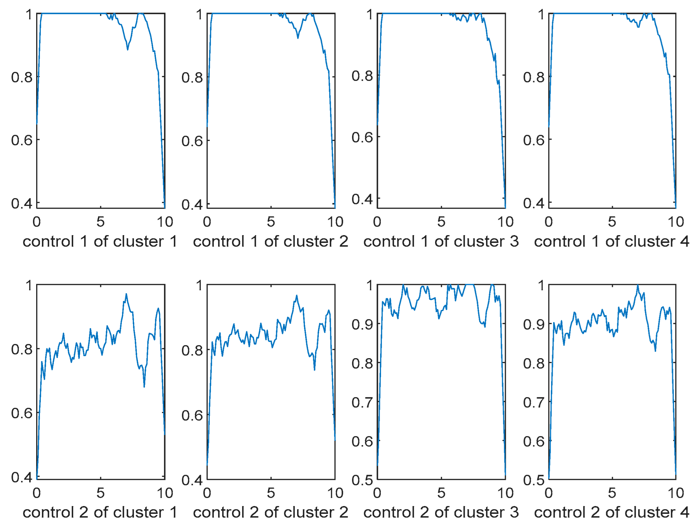
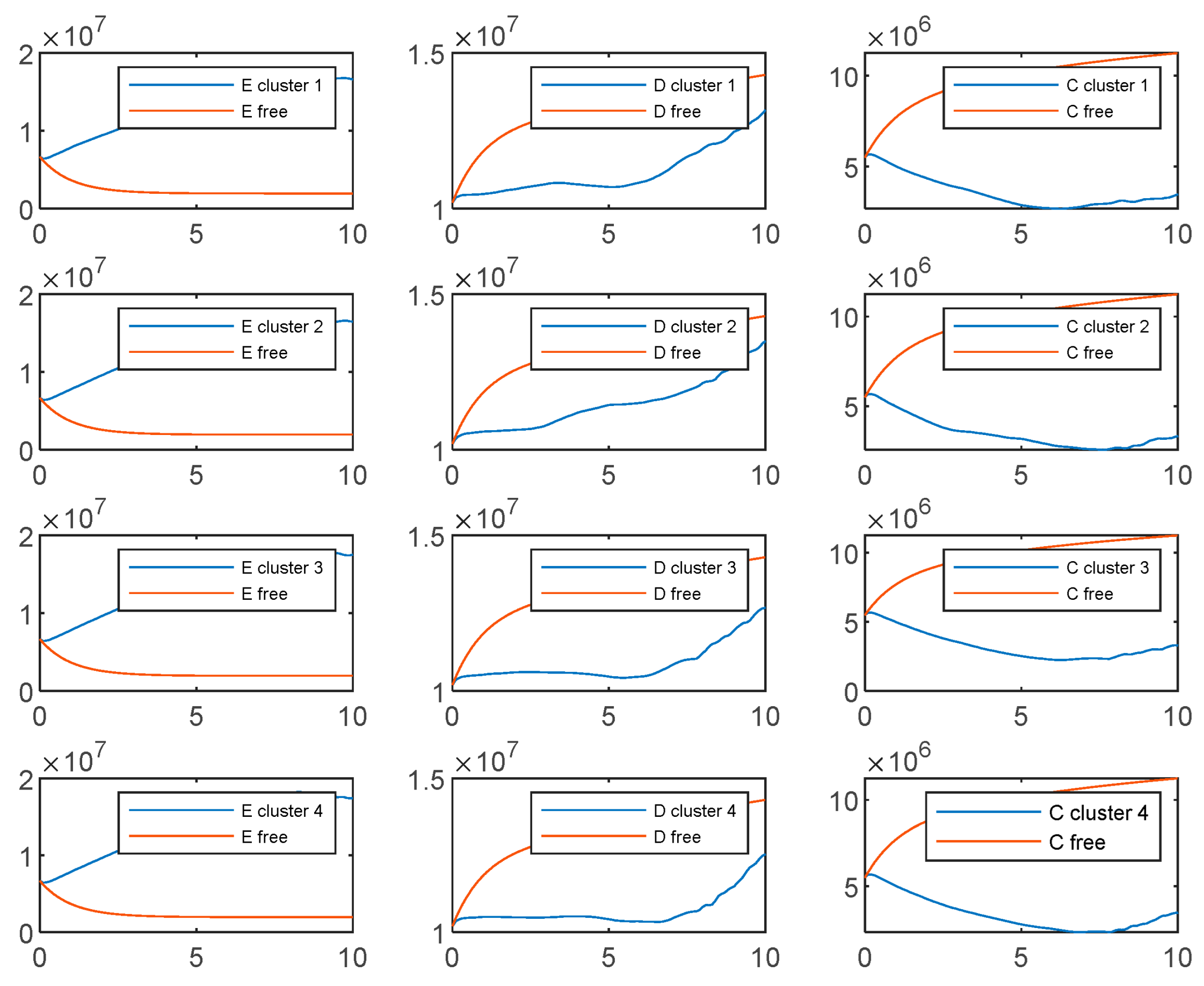
Considering the experimental results shown in the Figure A1, Figure A2, Figure A3 and Figure A4, we notice that the two soft clustering methods FCM and GMM give approximately the same groups (considering a simple permutation), so we extended the same remarks, conclusions, and recommendations to the other method.
(b)
The shapes of the front given in Figure 5 and those given in Figure 9 show that NSGA-II offers several highly non-dominated customized control strategies compared to MOFA.
(c)
According to Table 1 and Table 2, compared with NSGA-II, MOFA requires a large number of generations to achieve feasible and acceptable controls (60 generations for NSGA-II versus 1000 generations for MOFA).
We remark that MOFA-Soft-Cluster produces controls completely different to the ones produced via NSGA-II-Soft-Cluster. The sub-controls associated with compartment D, produced via MOFA-Soft-Cluster, are a symmetrical trapezoid of the support [2 years, 8 years], and the sub-controls associated with compartment C have very low cost along the control duration (they do not even consume 40% of the resources). So, what is wasted on one side is recovered on the other side. The sub-controls, associated with D, produced via NSGA-II-Soft-Cluster are a non-symmetrical trapezoid and they start by being too expensive and end up with a very low cost. Meanwhile, the sub-controls associated with C, produced via NSGA-II-Soft-Cluster, are too expensive from the beginning to the end (they consume between 80% and 100% of the resources). We cannot talk about the processing time because the size of the population and the size of the swarm influence the time complexity and we cannot establish a mathematical relation between the two sizes.

6.3. Single-Objective vs. Multi-Objective on the Control of the Dynamics of the Diabetic Population Problem (C2D2P)

In [19], the authors modeled the problem C2D2P in terms of the single-objective dynamic mathematical model. To solve these models, they used the Gumel method based on Pantriagin’s principle; the obtained control is represented in red in Figure A6. Since a control mobilizes human and material resources, it would be better if this control took as small values as possible. In this sense, Gumel was rejected because it takes very high values (these controls consume practically all resources). In our previous work [4], we used the bees algorithm (BA), firefly algorithm (FA), particle swarm algorithm (PSO), genetic algorithm (GA), moth swarm algorithm (MSA), stochastic fractal search (SFS), wind-driven optimization (WDO) and probabilistic bees algorithm (PBA); see Figure A6. The stochastic fractal search (SFS) method has shown an unprecedented ability to produce continuous, economical controls capable of alleviating socio-economic damage on a reasonable budget. Compared to a multi-objective strategy (introduced in this work), PSO, FA, GA, AWD, SBA, PBA, MWA and SFS propose the same strategies to control compartments C and D . When dealing with conflicting cost functions, a single solution is not reasonable because a solution that may be appropriate in one context may not be appropriate in another. The characteristics of patients in D are not similar to the ones of C . For example, 40 min of running combined with 2 g of medication may regulate the blood sugar of a compartment D patient, but this solution may not be suitable for a compartment C patient (whose complications prevent them from running), and 40 min of walking plus 6 g of medication may prove more appropriate.

6.4. Sensitivity of the Proposed System

To study the sensitivity of the controls obtained using the proposed model + NSGA-II + FCM, we applied Gaussian perturbations to the controls obtained using this system; this noise was generated between 0.001 and 0.3.
Figure A7, Figure A8, Figure A9, Figure A10, Figure A11 and Figure A12 show the comparisons obtained for certain noise values; see Appendix B as well. For Gaussian perturbations between 0.001 and 0.1, there was almost no change in the compartments. For Gaussian perturbations between 0.12 and 0.3, changes were noted in compartment D and small changes were noted in compartment C (the number of diabetics increases very rapidly compared with the case of optimal control developed in this work). This is normal, since the values taken by the control are between 0 and 1, and when almost 30% change is applied, the control changes; subsequently, the behavior of the compartments also changes.
In the end, we can say that the proposed approach is consistent when it comes to small Gaussian noise.
At the end of this section, we prefer not to make technical comparisons between the two types of strategies offered by the four systems because a choice may be appropriate in one context while it may be bad in another context. When there is a multi-objective problem, the role of the data scientist is the modeling of the studied phenomenon, the numerical simulation and the structuring of the control space. Then, it is left to the medical experts to choose what suits them according to their requirements and availability.

7. Conclusions

Single-objective mathematical modeling was previously used for controlling the dynamics of populations having one or more chronic diseases, in particular controlling the dynamics of the diabetic population. Unfortunately, the controls obtained make no distinction between the different compartments. In this work, we introduce a multi-objective approach that implements a multi-objective optimization model, population-based metaheuristics (NSGA-II and MOFA), flexible unsupervised learning (FCM and GMM), polynomial interpolation and FFT convolution for the problem of controlling the diabetic population. The optimization model implements two objective functions: one for diabetics without complications and another for diabetics with complications. To avoid solving large constraint systems, our approach calls the Euler–Cauchy method once we have a premature approximation of the control. The parameters of the heuristic methods are chosen experimentally. To clean up the resulting controls from noise due to successive approximations, we used a fast Fourier transform with a kernel size of 9 × 9 , chosen experimentally. Since it is difficult for a diabetes specialist to choose the right control for their use, from the Pareto front, we used two soft clustering methods to structure the solution space, where the optimal number of clusters was selected on the basis of the silhouette criterion. The controls produced enabled the evacuation of the compartments of diabetics with and without complications, except that towards the end of the control period, we noticed a small increase in these compartments, a problem we can solve by adding more control approximation points. In addition, the controls produced are customized because the required resources to control the diabetics without complications are totally different from the required resources to control the diabetics with complications. In addition, the multi-objective strategy permits us to save a good number of resources. In the future, we will use variational Bayes techniques to estimate the parameters of the multi-objective model in order to remedy sampling-related problems. To improve the control quality, we will use hybrid metaheuristics (MFOA + NSGA) while introducing the notion of attractiveness during crossover or mutation. In addition, we will introduce the fractional version of the multi-objective model to handle more information about the dynamics of the diabetic population.

Author Contributions

Conceptualization, K.E.M.; Methodology, K.E.M. and V.P.; Validation, A.C.; Investigation, K.E.M. and A.C.; Data curation, K.E.M., H.B., S.C. and M.C.; Writing – original draft, K.E.M. and A.E.O.; Writing – review & editing, V.P., A.C. and A.O. All authors have read and agreed to the published version of the manuscript.

Funding

This research received no external funding.

Data Availability Statement

Data are available under request.

Acknowledgments

This work was supported by the Ministry of National Education, Professional Training, Higher Education and Scientific Research (MENFPESRS), the Digital Development Agency (DDA) and the CNRST of Morocco (Nos. Alkhawarizmi/2020/23).

Conflicts of Interest

The authors declare no conflict of interest.

Appendix A

Figure A1. Controls pair obtained via GMM applied to the Pareto front produced via NSGA-II.
Mathematics 11 02957 g0a1
Figure A2. Compartments obtained using different controls produced via GMM applied to the Pareto front produced via NSGA-II.
Mathematics 11 02957 g0a2
Figure A3. Controls pair obtained via GMM applied to the Pareto front produced via MOFA.
Mathematics 11 02957 g0a3
Figure A4. Compartments obtained when introducing different controls, produced via GMM applied to the Pareto front produced via MOFA applied to the model (4).
Mathematics 11 02957 g0a4
Figure A5. Selection of the optimal number of clusters based on the silhouette criteria of groups obtained via FCM.
Mathematics 11 02957 g0a5
Figure A6. Gumel control and meta-heuristics controls for the Bouteyeb model.
Mathematics 11 02957 g0a6

Appendix B

Figure A7. Compartments obtained when introducing different controls, produced via FCM, applied to the Pareto front produced via NSGA-II, for which we added Gaussian noise from [0, 0.05].
Mathematics 11 02957 g0a7
Figure A8. Compartments obtained when introducing different controls, produced via FCM, applied to the Pareto front produced via NSGA-II, for which we added Gaussian noise from [0, 0.1].
Mathematics 11 02957 g0a8
Figure A9. Compartments obtained when introducing different controls, produced via FCM, applied to Pareto front produced via NSGA-II, for which we added Gaussian noise from [0, 0.15].
Mathematics 11 02957 g0a9
Figure A10. Compartments obtained when introducing different controls, produced via FCM applied to the Pareto front produced via NSGA-II, for which we added Gaussian noise from [0, 0.2].
Mathematics 11 02957 g0a10
Figure A11. Compartments obtained when introducing different controls, produced via FCM applied to the Pareto front produced via NSGA-II, for which we added Gaussian noise from [0, 0.25].
Mathematics 11 02957 g0a11
Figure A12. Compartments obtained when introducing different controls, produced via FCM, applied to the Pareto front produced via NSGA-II, for which we added Gaussian noise from [0, 0.3].
Mathematics 11 02957 g0a12

References

  1. International Diabetes Federation (IDF). About—Diabetes. Available online: https://idf.org/about-diabetes/facts-figures (accessed on 1 May 2023).
  2. Abdellatif, E.O.; Karim, E.M.; Hicham, B.; Saliha, C. Intelligent local search for an optimal control of diabetic population dynamics. Math. Model. Comput. Simul. 2022, 14, 1051–1071. [Google Scholar] [CrossRef]
  3. El Moutaouakil, K.; Ahourag, A.; Chakir, S.; Kabbaj, Z.; Chellack, S.; Cheggour, M.; Baizri, H. Hybrid firefly genetic algorithm and integral fuzzy quadratic programming to an optimal Moroccan diet. Math. Model. Comput. 2023, 10, 338–350. [Google Scholar] [CrossRef]
  4. Ahourag, A.; El Moutaouakil, K.; Cheggour, M.; Chellak, S.; Baizri, H. Multiobjective optimization to optimal moroccan diet using genetic algorithm. Int. J. Eng. Model. 2023, 36, 67–79. [Google Scholar]
  5. Ahourag, A.; Chellak, S.; Cheggour, M.; Baizri, H.; Bahri, A. Quadratic programming and triangular numbers ranking to an optimal moroccan diet with minimal glycemic load. Stat. Optim. Inf. Comput. 2023, 11, 85–94. [Google Scholar]
  6. World Health Organisation. Definition and Diagnosis of Diabetes Mellitus and Intermediate Hyperglycemia; WHO: Geneva, Switzerland, 2016. [Google Scholar]
  7. IDF Diabetes Atlas, 9th ed.; International Diabetes Federation (IDF): Brussels, Belgium, 2019.
  8. Kouidere, A.; Khajji, B.; Balatif, O.; Rachik, M. A multi-age mathematical modeling of the dynamics of population diabetics with effect of lifestyle using optimal control. J. Appl. Math. Comput. 2021, 67, 375–403. [Google Scholar] [CrossRef]
  9. Abdellatif, E.O.; Karim, E.M.; Saliha, C.; Hicham, B. Genetic algorithms for optimal control of a continuous model of a diabetic population. In Proceedings of the 2022 IEEE 3rd International Conference on Electronics, Control, Optimization and Computer Science (ICECOCS), Fez, Morocco, 1–2 December 2022; pp. 1–5. [Google Scholar]
  10. Li, H.; Peng, R.; Wang, Z. On a diffusive susceptible-infected-susceptible epidemic model with mass action mechanism and birth-death effect: Analysis, simulations, and comparison with other mechanisms. SIAM J. Appl. Math. 2018, 78, 2129–2153. [Google Scholar] [CrossRef]
  11. Jin, H.Y.; Wang, Z.A. Global stabilization of the full attraction-repulsion keller-segel system. Discret. Contin. Dyn. Syst.—Ser. A 2020, 40, 3509–3527. [Google Scholar] [CrossRef] [Green Version]
  12. Yuan, M.; Li, Y.; Zhang, L.; Pei, F. Research on intelligent workshop resource scheduling method based on improved NSGA-II algorithm. Robot. Comput. Integr. Manuf. 2021, 71, 102141. [Google Scholar] [CrossRef]
  13. Ranganathan, S.; Surya Kalavathi, M.; Asir Rajan, C.C. Self-adaptive firefly algorithm based multi-objectives for multi-type FACTS placement. IET Gener. Transm. Distrib. 2016, 10, 2576–2584. [Google Scholar] [CrossRef]
  14. El Moutaouakil, K.; Yahyaouy, A.; Chellak, S.; Baizri, H. An optimized gradient dynamic-neuro-weighted-fuzzy clustering method: Application in the nutrition field. Int. J. Fuzzy Syst. 2022, 24, 3731–3744. [Google Scholar] [CrossRef]
  15. Boutayeb, A.; Chetouani, A. A population model of diabetes and pre-diabetes. Int. J. Comput. Math. 2007, 84, 57–66. [Google Scholar] [CrossRef]
  16. Mahata, A.; Mondal, S.P.; Alam, S.; Chakraborty, A.; De, S.K.; Goswami, A. Mathematical model for diabetes in fuzzy environment with stability analysis. J. Intell. Fuzzy Syst. 2019, 36, 2923–2932. [Google Scholar] [CrossRef]
  17. Ollerton, R.L. Application of optimal control theory to diabetes mellitus. Int. J. Control 1989, 50, 2503–2522. [Google Scholar] [CrossRef]
  18. Swan, G.W. An optimal control model of diabetes mellitus. Bull. Math. Biol. 1982, 44, 793–808. [Google Scholar] [CrossRef] [PubMed]
  19. Makroglou, A.; Karaoustas, I.; Li, J.; Kuang, Y. Delay differential equation models in diabetes modeling. Theor. Biol. Med. Model. 2009. Available online: https://d1wqtxts1xzle7.cloudfront.net/39776544/Delay_differential_equation_models_in_di20151107-11553-9sa4j7-libre.pdf?1446919153=&response-content-disposition=inline%3B+filename%3DDelay_differential_equation_models_in_di.pdf&Expires=1688109253&Signature=gzNPLMm9mZ3KYeZD9wfLLcKorB-7z3XPMW8kUnqEXooVDMVVRyQqbvUD1timDez8PEcjfkgNsLfYgASjLAJ~LP~rY5M7aihIVP5~wu4y5GR29sMBYBgTyszEQSG5g10Gt~LYiWgqbmPcrBXBP7Lcv5rkQkORQzTOxJhWoiRYadd8Hw6kBVlr4mjVPEMHxnQkgp6QEW-qlqF1FUKKG8pxI338xA~bkZDSiDKmGgzvjiEBBcBj3W1LCGQMZh1maPlnmVqaldj8n33dkCEXny5bM-yvEz64JsAJ6my3qC59kctUZR4YwI2rVjKTWhEN4dlD3ogdKkBRNA2bal4vQPpRCA__&Key-Pair-Id=APKAJLOHF5GGSLRBV4ZA (accessed on 1 May 2023).
  20. Derouich, M.; Boutayeb, A.; Boutayeb, W.; Lamlili, M. Optimal control approach to the dynamics of a population of diabetics. Appl. Math. Sci. 2014, 8, 2773–2782. [Google Scholar] [CrossRef]
  21. Gumel, A.B.; Shivakumar, P.N.; Sahai, B.M. A mathematical model for the dynamics of HIV-1 during the typical course of infection. Nonlinear Anal. Theory Methods Appl. 2001, 47, 1773–1783. [Google Scholar] [CrossRef]
  22. Yusuf, T.T. Optimal control of incidence of medical complications in a diabetic patients’ population. FUTA J. Res. Sci. 2015, 11, 180–189. [Google Scholar]
  23. Permatasari, A.H.; Tjahjana, R.H.; Udjiani, T. Existence and characterization of optimal control in mathematics model of diabetics population. J. Phys. Conf. Ser. 2018, 983, 012069. [Google Scholar] [CrossRef]
  24. Daud, A.A.M.; Toh, C.Q.; Saidun, S. Development and analysis of a mathematical model for the population dynamics of Diabetes Mellitus during pregnancy. Math. Model. Comput. Simul. 2020, 12, 620–630. [Google Scholar] [CrossRef]
  25. Kouidere, A.; Balatif, O.; Ferjouchia, H.; Boutayeb, A.; Rachik, M. Optimal control strategy for a discrete time to the dynamics of a population of diabetics with highlighting the impact of living environment. Discret. Dyn. Nat. Soc. 2019, 2019, 6342169. [Google Scholar] [CrossRef]
  26. Kouidere, A.; Labzai, A.; Ferjouchia, H.; Balatif, O.; Rachik, M. A new mathematical modeling with optimal control strategy for the dynamics of population of diabetics and its complications with effect of behavioral factors. J. Appl. Math. 2020, 2020, 1943410. [Google Scholar] [CrossRef]
  27. Ahourag, A.; El Moutaouakil, K.; Chellak, S.; Baizri, H.; Cheggour, M. Multi-criteria optimization for optimal nutrition of Moroccan diabetics. In Proceedings of the 2022 International Conference on Intelligent Systems and Computer Vision (ISCV), Fez, Morocco, 18–20 May 2022; pp. 1–6. [Google Scholar]
  28. El Moutaouakil, K.; Palade, V.; Safouan, S.; Charroud, A. FP-Conv-CM: Fuzzy probabilistic convolution C-means. Mathematics 2023, 11, 1931. [Google Scholar] [CrossRef]
  29. Bolduc, E.; Knee, G.C.; Gauger, E.M.; Leach, J. Projected gradient descent algorithms for quantum state tomography. npj Quantum Inf. 2017, 3, 44. [Google Scholar] [CrossRef] [Green Version]
  30. Auslender, A.; Teboulle, M. Lagrangian duality and related multiplier methods for variational inequality problems. SIAM J. Optim. 2000, 10, 1097–1115. [Google Scholar] [CrossRef]
  31. Föllmer, H.; Kabanov, Y.M. Optional decomposition and Lagrange multipliers. Financ. Stoch. 1997, 2, 69–81. [Google Scholar] [CrossRef] [Green Version]
  32. Rahman, Q.I.; Schmeisser, G. Characterization of the speed of convergence of the trapezoidal rule. Numer. Math. 1990, 57, 123–138. [Google Scholar] [CrossRef]
  33. Fleming, W.H.; Rishel, R.W. Deterministic and Stochastic Optimal Control; Springer: New York, NY, USA, 1975. [Google Scholar]
  34. Frigo, M.; Johnson, S.G. FFTW: An adaptive software architecture for the FFT. In Proceedings of the International Conference on Acoustics, Speech, Signal Processing, Seattle, WA, USA, 15 May 1998; Volume 3, pp. 1381–1384. [Google Scholar]
  35. Jawad, K.; Mahto, R.; Das, A.; Ahmed, S.U.; Aziz, R.M.; Kumar, P. Novel cuckoo search-based metaheuristic approach for deep learning prediction of depression. Appl. Sci. 2023, 13, 5322. [Google Scholar] [CrossRef]
  36. Ali, S.; Bhargava, A.; Saxena, A.; Kumar, P. A hybrid marine predator sine cosine algorithm for parameter selection of hybrid active power filter. Mathematics 2023, 11, 598. [Google Scholar] [CrossRef]
  37. Wang, Y.J.; Wang, G.G.; Tian, F.M.; Gong, D.W.; Pedrycz, W. Solving energy-efficient fuzzy hybrid flow-shop scheduling problem at a variable machine speed using an extended NSGA-II. Eng. Appl. Artif. Intell. 2023, 121, 105977. [Google Scholar] [CrossRef]
  38. Yazdinejad, A.; Dehghantanha, A.; Parizi, R.M.; Epiphaniou, G. An optimized fuzzy deep learning model for data classification based on NSGA-II. Neurocomputing 2023, 522, 116–128. [Google Scholar] [CrossRef]
  39. Rafati, N.; Hazbei, M.; Eicker, U. Louver configuration comparison in three Canadian cities utilizing NSGA-II. Build. Environ. 2023, 229, 109939. [Google Scholar] [CrossRef]
  40. Chen, H.; Feng, Z.; Liu, Y.; Chen, B.; Deng, T.; Qin, Y.; Xu, W. Multiobjective optimization of a 3D laser scanning scheme for engineering structures based on RF-NSGA-II. J. Constr. Eng. Manag. 2023, 149, 04022169. [Google Scholar] [CrossRef]
  41. Singh, M.K.; Choudhary, A.; Gulia, S.; Verma, A. Multi-objective NSGA-II optimization framework for UAV path planning in an UAV-assisted WSN. J. Supercomput. 2023, 79, 832–866. [Google Scholar] [CrossRef]
  42. Wang, D.; Wang, G.; Wang, H. Optimal lane change path planning based on the NSGA-II and TOPSIS algorithms. Appl. Sci. 2023, 13, 1149. [Google Scholar] [CrossRef]
  43. Nan, Y.; Zhang, H.; Zeng, Y.; Zheng, J.; Ge, Y. Faster and accurate green pepper detection using NSGA-II-based pruned YOLOv5l in the field environment. Comput. Electron. Agric. 2023, 205, 107563. [Google Scholar] [CrossRef]
  44. Li, S.; Zhou, H.; Xu, G. Research on optimal configuration of landscape storage in public buildings based on improved NSGA-II. Sustainability 2023, 15, 1460. [Google Scholar] [CrossRef]
  45. Wang, Z.; Shen, L.; Li, X.; Gao, L. An improved multi-objective firefly algorithm for energy-efficient hybrid flowshop rescheduling problem. J. Clean. Prod. 2023, 385, 135738. [Google Scholar] [CrossRef]
  46. Tiwari, A.; Chaturvedi, A. Automatic EEG channel selection for multiclass brain-computer interface classification using multiobjective improved firefly algorithm. Multimed. Tools Appl. 2023, 82, 5405–5433. [Google Scholar] [CrossRef]
  47. He, Y.; Peng, H.; Deng, C.; Dong, X.; Wu, Z.; Guo, Z. Reference point reconstruction-based firefly algorithm for irregular multi-objective optimization. Appl. Intell. 2023, 53, 962–983. [Google Scholar] [CrossRef]
  48. Ri, K.W.; Mun, K.H. Firefly algorithm hybridized with genetic algorithm for multi-objective integrated process planning and scheduling. Res. Sq. 2023. [Google Scholar] [CrossRef]
  49. Ahmadi, S.E.; Kazemi-Razi, S.M.; Marzband, M.; Ikpehai, A.; Abusorrah, A. Multi-objective stochastic techno-economic-environmental optimization of distribution networks with G2V and V2G systems. Electr. Power Syst. Res. 2023, 218, 109195. [Google Scholar] [CrossRef]
  50. Li, J.; Sun, G.; Wang, A.; Zheng, X.; Chen, Z.; Liang, S.; Liu, Y. Multi-objective sparse synthesis optimization of concentric circular antenna array via hybrid evolutionary computation approach. Expert Syst. Appl. 2023, 231, 120771. [Google Scholar] [CrossRef]
  51. Srinivasan, B.; Venkatesan, R.; Aljafari, B.; Kotecha, K.; Indragandhi, V.; Vairavasundaram, S. A novel multicriteria optimization technique for VLSI floorplanning based on hybridized firefly and ant colony systems. IEEE Access 2023, 11, 14677–14692. [Google Scholar] [CrossRef]
  52. Shou, S.; Luo, H.; Wang, X.; Li, Y.; Hu, J.; Su, L. Optimal configuration of power quality control device for new distribution network based on firefly algorithm. In Proceedings of the 2023 Panda Forum on Power and Energy (PandaFPE), Chengdu, China, 27–30 April 2023; pp. 872–876. [Google Scholar]
  53. Athisayam, A.; Kondal, M. Fault feature selection for the identification of compound gear-bearing faults using firefly algorithm. Int. J. Adv. Manuf. Technol. 2023, 125, 1777–1788. [Google Scholar] [CrossRef]
  54. El Moutaouakil, K.; Touhafi, A. A new recurrent neural network fuzzy mean square clustering method. In Proceedings of the 2020 5th International Conference on Cloud Computing and Artificial Intelligence: Technologies and Applications (CloudTech), Marrakesh, Morocco, 24–26 November 2020; pp. 1–5. [Google Scholar] [CrossRef]
Figure 1. Pareto front concept.
Mathematics 11 02957 g001
Figure 2. NSGA-II algorithm schematic diagram.
Mathematics 11 02957 g002
Figure 3. The MOFA algorithm schematic diagram.
Mathematics 11 02957 g003
Figure 4. Pareto front produced via NSGA-II applied to the model 4 .
Mathematics 11 02957 g004
Figure 5. (a) The set of controls u 1 extracted from the Pareto front produced via NSGA-II applied to model (4). (b) The set of controls u 2 extracted from the Pareto front produced via NSGA-II applied to model (4).
Mathematics 11 02957 g005aMathematics 11 02957 g005b
Figure 6. Control pairs, over 10 years, obtained via FCM applied to the Pareto front produced via NSGA-II.
Mathematics 11 02957 g006
Figure 7. Compartments obtained when introducing different controls, produced via FCM applied to the Pareto front produced via NSGA-II, in model (4).
Mathematics 11 02957 g007
Figure 8. Pareto front produced via MOFA applied to the model 4 .
Mathematics 11 02957 g008
Figure 9. (a) The set of controls u 1 extracted from the Pareto front produced via MOFA applied to the model (4). (b) The set of controls u 2 extracted from the Pareto front produced via MOFA applied to the model (4).
Mathematics 11 02957 g009aMathematics 11 02957 g009b
Figure 10. Controls pair obtained via FCM applied to the Pareto front produced via MOFA.
Mathematics 11 02957 g010
Figure 11. Compartments obtained when introducing different controls, produced via FCM applied to the Pareto front produced via MOFA, in the model (4).
Mathematics 11 02957 g011
Table 1. NSGA-II configuration.
Option [12]Configuration
Crossover operatorNew_indiv = indiv1 + rand × atio × (indiv2 − indiv1)
Crossover ratio0.8
Number of iterations60
Mutation ratioadaptive feasible
Table 2. MOFA configuration.
Option [13]Configuration
Maximum number of iterations1000
Swarm size25
Light absorption coefficient1
Attraction coefficient base value2
Mutation coefficient0.2
Mutation coefficient damping ratio0.98
Table 3. Multi-objective control strategy vs. single-objective control strategy.
Cluster 1Cluster 2Cluster 3Cluster 4
Multi-objective vs. single-objectiveu13%4%4%4%
u214%6%18%11%
Disclaimer/Publisher’s Note: The statements, opinions and data contained in all publications are solely those of the individual author(s) and contributor(s) and not of MDPI and/or the editor(s). MDPI and/or the editor(s) disclaim responsibility for any injury to people or property resulting from any ideas, methods, instructions or products referred to in the content.

