Article

A Dual Rumor Spreading Model with Consideration of Fans versus Ordinary People

1
Faculty of Science, Yibin University, Yibin 644000, China
2
Department of Mathematics, China Three Gorges University, Yichang 443002, China
3
Institute of Intelligence Science and Engineering, Shenzhen Polytechnic, Shenzhen 518055, China
4
School of Mathematics and Information Science, Shandong Technology and Business University, Yantai 264005, China
5
School of Mathematical and Computational Science, Hunan University of Science and Technology, Xiangtan 411201, China
*
Author to whom correspondence should be addressed.
Mathematics 2023, 11(13), 2958; https://doi.org/10.3390/math11132958
Submission received: 26 May 2023 / Revised: 27 June 2023 / Accepted: 29 June 2023 / Published: 3 July 2023

Abstract

:
The spread of rumors in online social networks (OSNs) has caused a serious threat to the normal social order. In order to describe the rumor-spreading dynamics in OSNs during emergencies, a novel model with consideration of fans versus ordinary people is proposed in this paper. In contrast to previous studies, we consider the case that two rumors exist simultaneously. It is assumed that one is an entertainment rumor that fans care about, and the other is a common rumor. First, we derive the mean-field equations that describe the dynamics of this dual rumor propagation model and obtain the threshold parameter. Secondly, after finding the necessary and sufficient conditions for the existence of equilibriums, we examine the equilibrium’s local and global stability. Finally, simulations are used to explain how various parameters affect the process of spreading rumors.

1. Introduction

One common definition of a rumor is an unconfirmed statement annotation on issues, events, or items of public interest. It is one of the most important forms of social communication. One way to study this topic is to use epidemic models such as SI, SIR, and SIS, because rumor spreading is very similar to epidemic diffusion. The earliest example is the D-K model proposed by Daley and Kendall [1]. In this model, the authors divided people into three classes: people who have not heard of the rumor, people who spread the rumor, and people who know but will not spread the rumor. From then on, various rumor spreading models have been proposed to improve the traditional epidemic models, such as the SIS model [2], the SIR model [3], the SIR¨CUA model [4], the SEIR model [5], and the ILSR model [6]. Some recent references are listed below for the 2IS2R model [7], SICR model [8], time delay model [9], stochastic model [10,11], and models that consider the influence mechanism [12,13]. One can also consult works that take into account psychological factors [14], the forgetting mechanism [15,16,17,18], the trust mechanism [19], the existence of debunking [20], and wise men with knowledge [21,22].
In an actual social network, numerous rumors may coexist, with multiple messages passing simultaneously and influencing one another. Rumors with similar content may reinforce each other, whereas rumors with content that is different from one another may suppress one another. In the following, some research on dual rumor models is introduced. Trpevski et al. [23] investigated the co-propagation of two rumors in social networks by expanding the traditional SIS rumor propagation model and establishing an interactive double rumor model. The authors gave the two models distinct communication states and assumed that the first rumor would be accepted first. Wang et al. [24] analyzed the occurrence of dual rumors and presented a 2S12R double rumor propagation model. It was assumed that each person could only spread one of the two rumors at a time. They also considered the situation of those who left the region, as well as newcomers to the population. Based on the theory of rumor propagation dynamics, Ji et al. [25] studied the propagation mechanism of anti-rumor dynamics. It was speculated that there are two hostile rumors in the network, and anti-rumors occupy a dominant position in the propagation process. The authors recorded the time at which the counter-rumors entered the web and conducted a comprehensive simulation experiment on the time threshold. Fu Mingming et al. [26] constructed WS and BA networks, ran a numerical simulation, and compared the influence of the basic regeneration number on the rumor propagation process. To investigate the dynamic mechanism of the interaction between the old and new rumor on a network, Zan Yongli [27] developed both the DSIR and C-DSIR rumor propagation models. Additionally, the authors investigated the influence of rumor publishers, network topology parameters, and the time interval between old and new rumors on the propagation process.
According to previous research, there are numerous human behaviors that influence rumor propagation. People are worried about the spread of entertainment rumors, especially those from young people. Entertainment rumors refer to rumors about popular singers, movie stars, soccer players, and internet celebrities, among others. Ordinary rumors refer to social hot spots or street gossip. Young people are full of enthusiasm for celebrity-related affairs. In some instances, idol worshipers are happy to circulate amusement rumors about idols. A survey found that 94% of the more than 100 elementary and middle school students in a city have purchased idols’ photographs, posters, photo albums, and other similar items, and 57% of them do so on a regular basis. Some research explains from the economical [28,29], sociological [30,31], and psychological [32,33] perspectives why young people are so keen to follow celebrities.
Understanding the differential dissemination mechanisms between general rumors and entertainment rumors among fans and non-fans is crucial in the era of pervasive information sharing. While prior research has explored the influence of rumors on individuals’ beliefs and behaviors, there is limited understanding of how these rumors spread differently within fan communities and among the general population. By examining these distinct dissemination mechanisms, this study aims to shed light on the underlying factors that drive the transmission of rumors and the role of fandom in shaping their spread. The findings will provide valuable insights into effective rumor management strategies and contribute to our understanding of information diffusion in the digital age.
Our main results and contributions are summarized as follows. In this paper, we consider the case where an entertainment rumor and a common rumor exist simultaneously, and there is a certain number of fans in the audience. Theoretical research is conducted on the existence of equilibriums and their stability. The outcomes of the simulation demonstrate that, given a sufficient number of fans and their level of enthusiasm, entertainment rumors can effectively suppress ordinary rumors. This might make sense, since when there is major social information on the web that the public authority does not believe it should spread, the media can deliver gossip about top stars to stifle the spread of the previous social news.
The rest of this paper is organized as follows. In Section 2, we derive the mean-field equations that describe the dynamics of this dual rumor propagation model. The necessary and sufficient conditions for the existence of equilibriums are described in Section 3. Section 4 contains the computation of the threshold parameter and stability analysis for our model. Section 5 includes numerical simulations and sensitivity analysis of the parameters. Finally, our conclusions are presented in Section 6.

2. Problem Formulation and Preliminaries

Typically, ISR rumor propagation models divide people into three categories: spreader (S), stifler (R), and ignorant (I) [10]. The spreader has accepted the rumor and will spread it, while the stifler has accepted the rumor and decided not to propagate it. The ignorant group refers to people who did not hear the rumor.
Based on the influence of fans versus ordinary people and the existence of dual rumors, we assume that two rumors exist: rumor 1 is about entertainment, and rumor 2 is common. Furthermore, we divide people into five groups: I 1 denotes individuals who have not heard rumor 1, I 2 denotes individuals who have not heard rumor 2, S 1 denotes individuals who spread rumor 1, and S 2 denotes individuals who spread rumor 2, whereas R denotes individuals who are aware of the two rumors but will not spread them. The rumor propagation process can be shown in Figure 1, and the mean-field equation is illustrated in Equation (1).
d S 1 d t = α 1 I 1 S 1 + α 12 I 2 S 1 μ S 1 β 1 S 1 , d S 2 d t = α 2 I 2 S 2 μ S 2 β 2 S 2 , d I 1 d t = m θ μ I 1 α 1 I 1 S 1 , d I 2 d t = m ( 1 θ ) μ I 2 α 12 I 2 S 1 α 2 I 2 S 2 , d R d t = β 1 S 1 + β 2 S 2 μ R .
where each of the eight parameters is positive and their meanings are listed as below:
  • m: the coming rate of internet users;
  • θ : the percentage of fans among internet users, where 0 < θ < 1 ;
  • μ : the exit rate of each group;
  • α j : the transmission rate from I j to S j ( j = 1 , 2 );
  • α 12 : the cross-transmitted rate from I 2 to S 1 ;
  • β j : the forgetting rate of S j ( j = 1 , 2 ).
Remark 1.
We have the following assumptions. When I j contacts S j , the former may spread rumor j with a probability of α j ; an ordinary person may be interested in entertainment rumor 1 and spread it with a probability of α 12 ; fans are irrational, and thus they only care about rumor 1 and will not spread rumor 2; S j will change into R due to the forgetting mechanism [6,34]; the irrationality of fans and the rationality of ordinary people support the hypothesis that α 1 > α 12 ; and for the sake of mathematical argument, the exit rate of each group is supposed to be identical.
Let N ( t ) = S 1 ( t ) + S 2 ( t ) + I 1 ( t ) + I 2 ( t ) + R ( t ) . It can be derived from Equation (1) that
d N d t = m μ N ( t ) .
Thus, we have N ( t ) < m μ . In what follows, we will study the model in Equation (1) in the following feasible region:
Ω = ( S 1 , S 2 , I 1 , I 2 , R ) R 5 + : 0 S 1 ( t ) + S 2 ( t ) + I 1 ( t ) + I 2 ( t ) + R ( t ) m μ .

3. Existence of Equilibriums

In this section, we investigate whether the equilibriums of Equation (1) exist. It is straightforward to find the rumor-demise equilibrium E 0 = ( S 1 , S 2 , I 1 , I 2 , R ) = ( 0 , 0 , m θ μ , m ( 1 θ ) μ , 0 ) . We shall start with a necessary condition for the existence of rumor-permanence equilibrium:
Proposition 1.
If the rumor-permanence equilibrium E * = ( S 1 * , S 2 * , I 1 * , I 2 * , R * ) of the model in Equation (1) exists, then it must have the following form:
I 2 * = μ + β 2 α 2 , I 1 * = μ + β 1 α 12 I 2 * α 1 , S 1 * = m θ μ + β 1 α 12 I 2 * μ α 1 , S 2 * = m ( 1 θ ) α 2 I 2 * α 12 m θ α 2 ( μ + β 1 α 12 I 2 * ) + μ ( α 12 α 1 ) α 1 α 2 , R * = β 1 S 1 * + β 2 S 2 * μ .
Proof. 
By definition of the rumor-permanence equilibrium, it is required that S 1 * , S 2 * , I 1 * , I 2 * , R * > 0 and
α 1 I 1 * S 1 * + α 12 I 2 * S 1 * μ S 1 * β 1 S 1 * = 0 , α 2 I 2 * S 2 * μ S 2 * β 2 S 2 * = 0 , m θ μ I 1 * α 1 I 1 * S 1 * = 0 , m ( 1 θ ) μ I 2 * α 12 I 2 * S 1 * α 2 I 2 * S 2 * = 0 , β 1 S 1 * + β 2 S 2 * μ R * = 0 .
By solving Equation (3), we can find the proof for this proposition. □
The last proposition suggests that the model in Equation (1) has at most one rumor-permanence equilibrium. In what follows, the existence of this rumor-permanence equilibrium will be considered. We will present a sufficient and necessary condition such that S 1 * , S 2 * , I 1 * , I 2 * , and R * , given in Equation (2), are all positive.
Theorem 1.
Equation (1) has a rumor-permanence equilibrium E * = ( S 1 * , S 2 * , I 1 * , I 2 * , I * ) if and only if
μ ( μ + β 1 ) m θ α 1 μ α 12 < μ + β 2 α 2 < b b 2 4 a c 2 a ,
with
a = μ ( α 12 α 1 ) α 1 , b = m μ ( 1 α 1 1 α 12 ) ( μ + β 1 ) , c = m ( 1 θ ) μ + β 1 α 12 .
Proof. 
To obtain a rumor-permanence equilibrium with the form in Equation (2), we only need to ensure I 1 * , S 1 * , S 2 * > 0 ; that is, it is required that
I 2 * > μ ( μ + β 1 ) m θ α 1 μ α 12 , I 2 * < μ + β 1 α 12 , ϕ ( I 2 * ) > 0 .
with ϕ ( t ) = m ( 1 θ ) t + m θ t μ + β 1 α 12 + μ ( α 12 α 1 ) α 1 . Under the assumption that α 1 > α 12 , the graph of the function ϕ ( t ) is presented in Figure 2. Note that I 2 * is positive by definition, and we obtain that the relation in Equation (6) holds if and only if
μ ( μ + β 1 ) m θ α 1 0 , I 2 * < t * .
or
μ ( μ + β 1 ) m θ α 1 > 0 , μ ( μ + β 1 ) m θ α 1 μ α 12 < I 2 * < t * ,
where t * = b b 2 4 a c 2 a , with a, b, and c given in Equation (5). Thus, we have proven this theorem. □

4. Stability Analysis of the Rumor-Spreading Model

4.1. The Threshold Parameter R 0

We will first calculate the threshold parameter R 0 of the model in Equation (1) with the next-generation matrix method [35].
Let X = ( S 1 ( t ) , S 2 ( t ) , I 1 ( t ) , I 2 ( t ) , R ( t ) ) . The model in Equation (1) can be rewritten as
d X d t = F ( X ) V ( X )
where
F ( X ) = α 1 I 1 S 1 + α 12 I 2 S 1 α 2 I 2 S 2 0 0 0 ,
V ( X ) = μ S 1 + β 1 S 1 , μ S 2 + β 2 S 2 , m θ + μ I 1 + α 1 I 1 S 1 , m ( 1 θ ) + μ I 2 + α 12 I 2 S 1 + α 2 I 2 S 2 , β 1 S 1 β 2 S 2 + μ R . .
The Jacobian matrices of F ( X ) and V ( X ) at the rumor-free equilibrium E 0 = ( 0 , 0 , m θ μ , m ( 1 θ ) μ , 0 ) are
D F ( E 0 ) = F 0 0 0 , D V ( E 0 ) = V 0 J 1 J 2 ,
with
F = 1 μ α 1 m θ + α 12 m ( 1 θ ) 0 0 α 2 m ( 1 θ ) ,
V = μ + β 1 0 0 μ + β 2 .
The threshold parameter R 0 is defined as the spectral radius of the matrix F V 1 ; that is, we have
R 0 = ρ ( F V 1 ) = m a x α 1 m θ + α 12 m ( 1 θ ) μ ( μ + β 1 ) , α 2 m ( 1 θ ) μ ( μ + β 2 ) .
Stability analysis of the model in Equation (1) will be conducted below. We point out that the Jacobian matrix of Equation (1) at point E = ( S 1 , S 2 , I 1 , I 2 , R ) is
J ( E ) = α 1 I 1 + α 12 I 2 μ β 1 0 α 1 S 1 α 12 S 1 0 0 α 2 I 2 μ β 2 0 α 2 S 2 0 α 1 I 1 0 α 1 S 1 μ 0 0 α 12 I 2 α 2 I 2 0 μ α 12 S 1 α 2 S 2 0 β 1 β 2 0 0 μ .

4.2. Stability at the Rumor-Demise Equilibrium E 0

Theorem 2.
Let R 0 be defined in Equation (7). If R 0 < 1 , then the rumor-demise equilibrium E 0 of Equation (1) is locally asymptotically stable.
Proof. 
It follows from Equation (8) that the Jacobian matrix of Equation (1) at E 0 = ( 0 , 0 , m θ μ , m ( 1 θ ) μ , 0 ) is
J ( E 0 ) = α 1 m θ μ + α 12 m ( 1 θ ) μ μ β 1 0 0 0 0 0 α 2 m ( 1 θ ) μ μ β 2 0 0 0 α 1 m θ μ 0 μ 0 0 α 12 m ( 1 θ ) μ α 2 m ( 1 θ ) μ 0 μ 0 β 1 β 2 0 0 μ .
It can be derived that J ( E 0 ) has the following eigenvalues:
λ 1 = λ 2 = λ 3 = μ < 0 , λ 4 = α 1 m θ μ + α 12 m ( 1 θ ) μ μ β 1 , λ 5 = α 2 m ( 1 θ ) μ μ β 2 .
According to the assumption that R 0 < 1 , we can obtain that λ 4 < 0 ,   λ 5 < 0 . Hence, based on the Routh–Hurwitz criterion [36], the rumor-demise equilibrium E 0 of Equation (1) is locally asymptotically stable if R 0 < 1 .
Theorem 3.
Let R 0 be defined in Equation (7). If R 0 < 1 , then the rumor-demise equilibrium E 0 of Equation (1) is globally asymptotically stable.
Proof. 
The Lyapunov function-based method [36] is used to prove the global stability. Let V = I 1 m θ μ m θ μ ln I 1 m θ μ + I 2 m ( 1 θ ) μ m ( 1 θ ) μ ln I 2 m ( 1 θ ) μ + S 1 + S 2 .
Then, we conclude that V is positive definite with respect to point E 0 and
V ˙ = I 1 m θ μ · I 1 I 1 + I 2 m ( 1 θ ) μ · I 2 I 2 + S 1 + S 2 = 2 m θ μ I 1 ( m θ ) 2 μ · 1 I 1 + 2 m ( 1 θ ) μ I 2 [ m ( 1 θ ) ] 2 μ · 1 I 2 + S 1 m θ α 1 μ μ β 1 + m ( 1 θ ) μ α 12 + S 2 m ( 1 θ ) α 2 μ μ β 2
Under the assumption that R 0 < 1 , we find that V ˙ 0 . Furthermore, if V ˙ = 0 , then S 1 = 0 , S 2 = 0 , I 1 = m θ μ , and I 2 = m ( 1 θ ) μ . Thus, we have accomplished this proof. □

4.3. Stability at the Rumor-Permanence Equilibrium E *

Theorem 4.
The rumor-demise equilibrium E * of Equation (1) is locally asymptotically stable if it exists.
Proof. 
It follows from Equations (3) and (8) that
J ( E * ) = 0 0 α 1 S 1 * α 12 S 1 * 0 0 0 0 α 2 S 2 * 0 α 1 I 1 * 0 α 1 S 1 * μ 0 0 α 12 I 2 * α 2 I 2 * 0 μ α 12 S 1 * α 2 S 2 * 0 β 1 β 2 0 0 μ .
It is clear that J ( E * ) has one eigenvalue, where λ 1 = μ < 0 . Let
A 12 = α 1 S 1 * α 12 S 1 * 0 α 2 S 2 * ,   A 21 = α 1 I 1 * 0 α 12 I 2 * α 2 I 2 * ,   A 22 = α 1 S 1 * μ 0 0 μ α 12 S 1 * α 2 S 2 * .
We verify that other eigenvalues of J ( E * ) are roots of the equation A 21 A 12 + λ A 12 λ 2 E = 0 . This can restated as the other four eigenvalues of J ( E * ) are just roots of a fourth polynomial f ( λ ) with the next form:
λ 2 + μ + α 1 S 1 * λ + α 1 2 I 1 * S 1 * λ 2 + μ + α 12 S 1 * + α 2 S 2 * λ + α 12 2 I 2 * S 1 * + α 2 2 I 2 * S 2 * α 1 2 α 12 2 I 1 * I 2 * S 1 * .
It follows from Proposition A2 that all roots λ i of f ( λ ) satisfy R e ( λ i ) < 0 . According to the Routh–Hurwitz criterion [36], this proof is accomplished. □
Theorem 5.
The rumor-demise equilibrium E * of Equation (1) is globally asymptotically stable if it exists.
Proof. 
Similar to the proof of Theorem 3, we use the Lyapunov method [36]. We define the Lyapunov function as
V = S 1 S 1 * S 1 * ln S 1 S 1 * + S 2 S 2 * S 2 * ln S 2 S 2 * + I 1 I 1 * I 1 * ln I 1 I 1 * + I 2 I 2 * ln I 2 I 2 *
Through direct calculation, we can verify that V ( S 1 , S 2 , I 1 , I 2 ) is positive definite with respect to point E * . On the other hand, the derivative of V along solutions of Equation (1) is
V ˙ = S 1 S 1 * S 1 S 1 + S 2 S 2 * S 2 S 2 + I 1 I 1 * I 1 I 1 + I 2 I 2 * I 2 I 2 .
By substituting Equation (3) into V ˙ , we obtain
V ˙ = α 2 I 2 * S 2 * ( 2 I 2 I 2 * I 2 * I 2 ) + α 12 I 2 * S 1 * ( 2 I 2 I 2 * I 2 * I 2 ) + α 1 I 1 * S 1 * ( 2 I 1 I 1 * I 1 * I 1 ) μ ( I 2 I 2 * ) 2 I 2 μ ( I 1 I 1 * ) 2 I 1 0 .
Moreover, V ˙ = 0 implies that I 1 = I 1 * and I 2 = I 2 * . By substituting this into Equation (1), we obtain S 1 = S 1 * , S 2 = S 2 * , and R * = R . This proves the global stability of E * under the condition that it exists. □

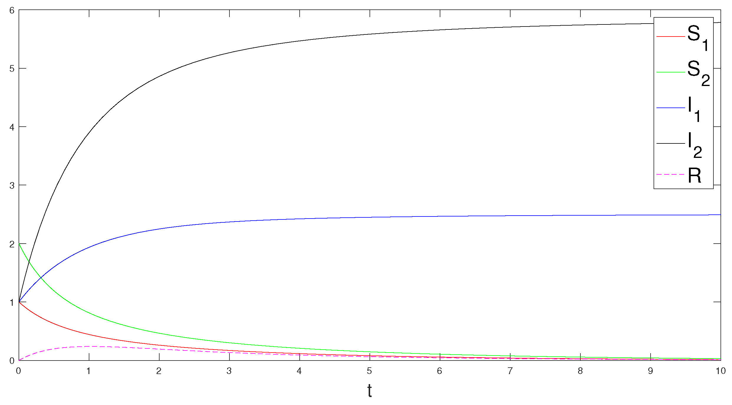
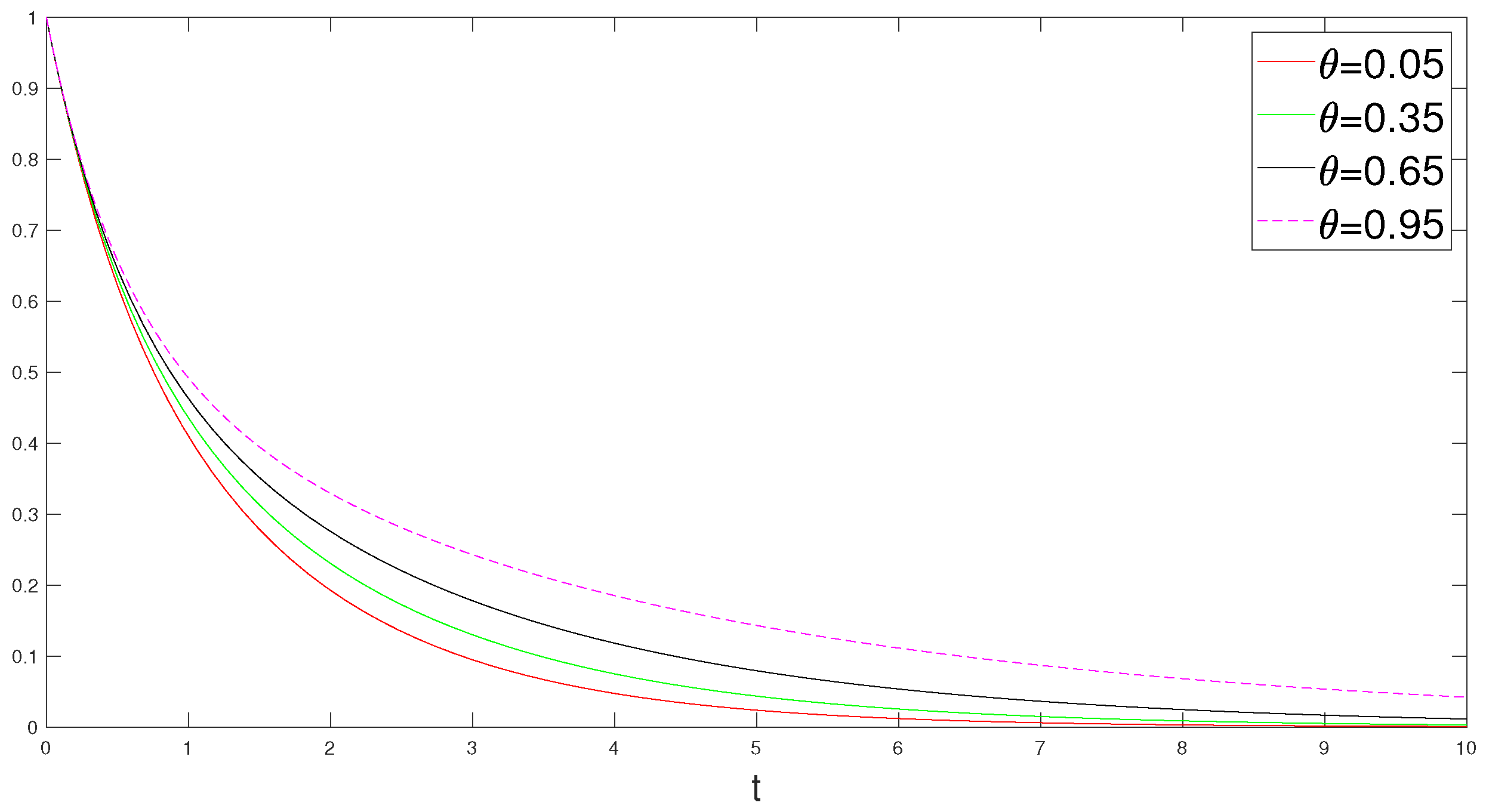
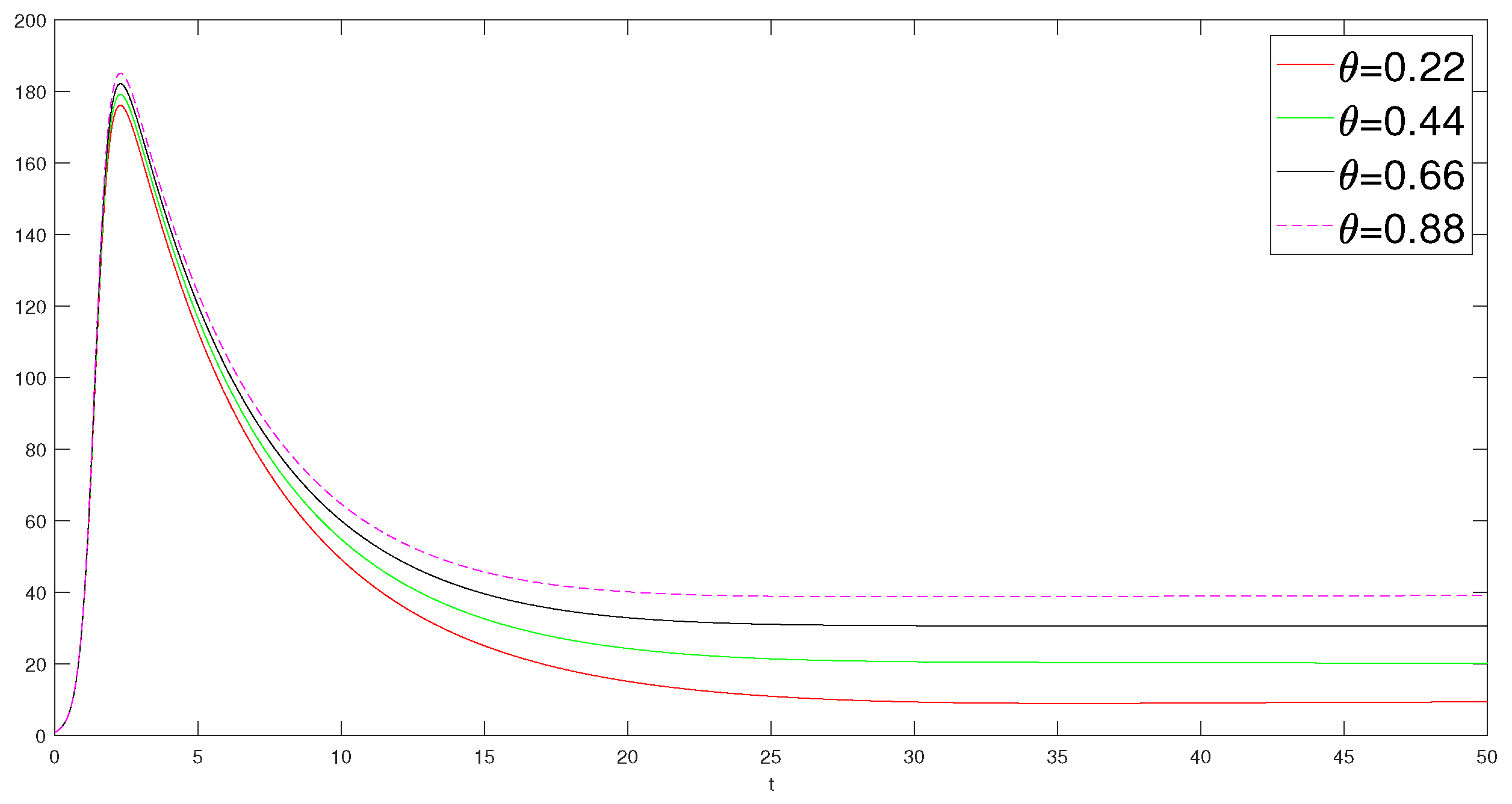
5. Numerical Simulations and Discussions

Numerical simulations are presented below to validate the analytical results in Section 4. Figure 3, Figure 4, Figure 5 and Figure 6 are used to exemplify that the rumor-demise equilibrium E 0 is asymptotically stable if R 0 < 1 . On the other hand, Figure 7, Figure 8 and Figure 9 illustrate the asymptotic stability of the rumor-demise equilibrium E * under the condition that it exists.
Figure 3 illustrates how the numbers of the five classes of individuals changed over time t if R 0 = 0.8046 < 1 . We assume that the number of five classes at time t 0 are S 1 ( 0 ) = 1 ,   S 2 ( 0 ) = 2 ,   I 1 ( 0 ) = 1 ,   I 2 ( 0 ) = 1 , and R ( 0 ) = 0 . As can be seen, S 1 and S 2 both decreased in a recursive manner until they reached zero. Additionally, I 1 and I 2 ,   R converged to their steady state as well.
To obtain Figure 4, we chose another set of parameters such that R 0 = 0.8333 < 1 and observed results similar to those in Figure 3. The differences between the two examples are as follows. According to Figure 3, more people cared about the common rumor (rumor 2) than the entertainment rumor (rumor 1) when the number of fans was lower than the number of ordinary people. However, if the number of fans was greater than the number of ordinary people, then the opposite is shown in Figure 4. This is because the percentage of fans determines how many people care about entertainment rumors.
Figure 5 describes how the number of those who spread rumor 1 changed over time t with the different fan rate θ . This figure also shows that the larger the fan rate θ , the greater the number of rumor 1 spreaders.
According to Figure 6, the number of people who spread rumor 2 fluctuated over time in accordance with the various fan rate θ . We can see that the number of rumor 2 spreaders decreased proportionally with parameter θ . Note that θ ranges over [0.05, 0.95] in Figure 5 and only ranges over [0.79, 0.95] in Figure 6 because we needed to ensure that R 0 < 1 .
Figure 7 illustrates how the numbers of the five classes of individuals varied over time t for R 0 = 42.85 > 1 . As shown in the figure, S 1 rapidly increased to the peak points and then decreased to a stable value slightly. On the other hand, S 2 gradually rose until it reached equilibrium. The figure also shows that in the equilibrium state, the number of people spreading the rumor was much higher than the number of people spreading rumor 2; that is to say, it is entirely possible for an entertainment rumor to suppress an ordinary rumor if the percentage of fans and their enthusiasm are sufficient.
Figure 8 and Figure 9 exemplify the sensitivity of S 1 and S 2 , respectively, with respect to parameter θ . The two numerical experiments demonstrate that in the early stages, rumors will spread quickly; that is, the number of rumor 1 spreaders and rumor 2 spreaders will rapidly rise until a major outbreak. Then, as a result of the forgetting mechanism, the two rumors are spread by fewer and fewer people until they reach equilibrium.

6. Conclusions

In this paper, we considered the case where an entertainment rumor and a common rumor existed simultaneously and there was a certain number of fans in the audience. The threshold parameter R 0 was obtained, and the asymptotic stability of the rumor-demise equilibrium E 0 was proven when R 0 < 1 . In addition, we presented the necessary and sufficient conditions for the existence of a rumor-permanence equilibrium E * and demonstrated that E * is both locally and globally stabilized when it exists. The simulation results demonstrated that it is entirely possible for entertainment rumors to suppress ordinary rumors if the percentage of fans and their enthusiasm are sufficient. This may explain why when there is a big social news on the Internet that the government does not want to spread, the media can release the rumors of top stars to suppress the spread of the former social news.

Author Contributions

Conceptualization, H.L.; Methodology, Y.Z. (Yuanyuan Zhang); Validation, Z.L. and Y.Z. (Yuxiao Zhao); Formal analysis, H.X., H.L. and Y.Z. (Yuxiao Zhao); Investigation, Z.L.; Writing—original draft, H.X.; Writing—review & editing, Y.Z. (Yuanyuan Zhang) and H.L.; Supervision, H.L. All authors contributed equally to this paper. All authors have read and agreed to the published version of the manuscript.

Funding

This work was supported by the specialized research fund of YiBin University (Grant No.412-2021QH027).

Data Availability Statement

The data that support the findings of this study are available from the corresponding author upon reasonable request.

Conflicts of Interest

The authors declare no conflict of interest.

Appendix A

In 1877, Routh [37] proposed a stability criterion that can determine whether a polynomial has only roots with negative real parts. Based on his work, we present the next proposition, which only deals with quartic polynomials:
Proposition A1.
Let f ( λ ) = λ 4 + p 3 λ 3 + p 2 λ 2 + p 1 λ + p 0 with all p i > 0 . Then, all roots of f ( λ ) have a negative real part if and only if k 1 > 0 and k 3 > 0 , where k i are given in Equation (A1).
Proof. 
Through application to [38], f ( λ ) only has roots with negative real parts if and only if all the elements in the first column of the Routh form H are positive, where
H = 1 p 2 p 0 p 3 p 1 k 1 k 2 k 3 0 k 4
and
k 1 = p 2 p 3 p 1 p 3 ,   k 2 = p 0 ,   k 3 = k 1 p 1 k 2 p 3 k 1 ,   k 4 = k 2 .
By definition, we have p 3 > 0 and k 4 > 0 . This proves this proposition. □
In what follows, we focus on a subset of quartic polynomials.
Proposition A2.
Assume that a i , b i > 0 ( i = 1 , 2 ) and 0 c < a 2 b 2 . Then, all the roots λ i of f ( λ ) satify R e λ i < 0 , where f ( λ ) : = λ 2 + a 1 λ + a 2 λ 2 + b λ + b 2 c .
Proof. 
Through a straightforward calculation, we have f ( λ ) = λ 4 + p 3 λ 3 + p 2 λ 2 + p 1 λ + p 0 with p 3 = b 1 + a 1 , p 2 = b 2 + a 1 b 1 + a 2 , p 1 = a 1 b 2 + a 2 b 1 , and p 0 = a 2 b 2 c . Thus, all the coefficients of f ( λ ) are positive. Let k 1 and k 3 be given in Equation (A1). It follows from Proposition A1 that we only need to verify k 1 , k 3 > 0 .
On the one hand, we can directly obtain p 2 p 3 p 1 > 0 , and thus k 1 > 0 . On the other hand, we have
k 3 = k 1 p 1 p 3 a 2 b 2 c k 1 = k 1 p 1 p 3 a 2 b 2 + p 3 c k 1 > k 1 p 1 p 3 a 2 b 2 k 1 > 0 .
The last inequality holds because for c = 0 , f ( λ ) = λ 2 + a 1 λ + a 2 λ 2 + b 1 λ + b 2 , whose roots λ i surely satisfy R e λ i < 0 . □

References

  1. Delay, D.; Kendall, D. Stochastic rumors. J. Inst. Math. Its Appl. 1965, 1, 42–55. [Google Scholar]
  2. Zhu, L.; Guan, G.; Li, Y. Nonlinear dynamical analysis and control strategies of a network-based SIS epidemic model with time delay. Appl. Math. Model. 2019, 70, 512–531. [Google Scholar] [CrossRef]
  3. Wang, J.; Jiang, H.; Ma, T.; Hu, C. Global dynamics of the multi-lingual SIR rumor spreading model with cross-transmitted mechanism. Chaos Solitons Fractals 2019, 126, 148–157. [Google Scholar] [CrossRef]
  4. Kabir, K.A.; Kuga, K.; Tanimoto, J. Analysis of SIR epidemic model with information spreading of awareness. Chaos Solitons Fractals 2018, 119, 118–125. [Google Scholar] [CrossRef]
  5. Zhou, Y.; Wu, C.; Zhu, Q.; Xiang, Y.; Loke, S.W. Rumor Source Detection in Networks Based on the SEIR Model. IEEE Access 2019, 7, 45240–45258. [Google Scholar] [CrossRef]
  6. Yang, A.; Huang, X.; Cai, X.; Zhu, X.; Lu, L. ILSR rumor spreading model with degree in complex network. Phys. A Stat. Mech. Its Appl. 2019, 531, 12–18. [Google Scholar] [CrossRef]
  7. Li, J.; Jiang, H.; Yu, Z.; Hu, C. Dynamical analysis of rumor spreading model in homogeneous complex networks. Appl. Math. Comput. 2019, 359, 374–385. [Google Scholar] [CrossRef]
  8. Li, J.; Ren, N.; Jin, Z. An SICR rumor spreading model in heterogeneous networks. Discret. Contin. Dyn. Syst.-B 2020, 25, 1497–1515. [Google Scholar] [CrossRef] [Green Version]
  9. Zhu, L.; Huang, X. SIS Model of Rumor Spreading in Social Network with Time Delay and Nonlinear Functions. Commun. Theor. Phys. 2020, 72, 015002. [Google Scholar] [CrossRef]
  10. Nekovee, M.; Moreno, Y.; Bianconi, G.; Marsili, M. Theory of rumour spreading in complex social networks. Phys. A Stat. Mech. Its Appl. 2007, 374, 457–470. [Google Scholar] [CrossRef] [Green Version]
  11. Huo, L.; Chen, X. Near-optimal control of a stochastic rumor spreading model with Holling II functional response function and imprecise parameters. Chin. Phys. B 2021, 12, 47–59. [Google Scholar] [CrossRef]
  12. Liu, C.; Zhan, X.-X.; Zhang, Z.-K.; Sun, G.-Q.; Hui, P.M. How events determine spreading patterns: Information transmission via internal and external influences on social networks. New J. Phys. 2015, 17, 113045. [Google Scholar] [CrossRef]
  13. Qiu, L.; Jia, W.; Niu, W.; Zhang, M.; Liu, S. SIR-IM: SIR rumor spreading model with influence mechanism in social networks. Soft Comput. 2020, 25, 13949–13958. [Google Scholar] [CrossRef]
  14. Xu, H.; Li, T.; Liu, X.; Liu, W.; Dong, J. Spreading dynamics of an online social rumor model with psychological factors on scale-free networks. Phys. A Stat. Mech. Its Appl. 2019, 525, 234–246. [Google Scholar] [CrossRef]
  15. Deng, S.; Li, W. Spreading dynamics of forget-remember mechanism. Phys. Rev. E 2017, 95, 042306. [Google Scholar] [CrossRef]
  16. Wang, J.; Li, M.; Wang, Y.; Zhou, Z.; Zhang, L. The influence of oblivion-recall mechanism and loss-interest mechanism on the spread of rumors in complex networks. Int. J. Mod. Phys. C 2019, 30, 1950075. [Google Scholar]
  17. Cao, B.; Han, S.-H.; Jin, Z. Modeling of knowledge transmission by considering the level of forgetfulness in complex networks. Phys. A Stat. Mech. Its Appl. 2016, 451, 277–287. [Google Scholar] [CrossRef]
  18. Ding, H.; Xie, L. Simulating rumor spreading and rebuttal strategy with rebuttal forgetting: An agent-based modeling approach. Phys. A Stat. Mech. Its Appl. 2023, 612, 128488. [Google Scholar] [CrossRef]
  19. Wang, Y.-Q.; Yang, X.-Y.; Han, Y.-L.; Wang, X.-A. Rumor Spreading Model with Trust Mechanism in Complex Social Networks. Commun. Theor. Phys. 2013, 59, 510–516. [Google Scholar] [CrossRef]
  20. Tian, Y.; Deng, X. Rumor spreading model with considering debunking behavior in emergencies. Appl. Math. Comput. 2019, 363, 127–138. [Google Scholar] [CrossRef]
  21. Hu, Y.; Pan, Q.; Hou, W.; He, M. Rumor spreading model considering the proportion of wisemen in the crowd. Phys. A Stat. Mech. Its Appl. 2018, 505, 1084–1094. [Google Scholar] [CrossRef]
  22. Huo, L.; Song, N. Dynamical interplay between the dissemination of scientific knowledge and rumor spreading in emergency. Phys. A Stat. Mech. Its Appl. 2016, 461, 73–84. [Google Scholar] [CrossRef]
  23. Trpevski, D.; Tang, W.; Kocarev, L. Model for rumor spread in gover networks. Phys. Rev. E 2010, 81, 156–172. [Google Scholar] [CrossRef]
  24. Wang, J.; Zhao, L.; Huang, R. 2SI2R rumor spreading model inhomogeneous networks. Phys. A Stat. Mech. Its Appl. 2014, 413, 153–161. [Google Scholar] [CrossRef]
  25. Ji, K.; Liu, J.; Xiang, G. Anti-rumor dynamics and emergence of the timing threshold on complex network. Phys. A Stat. Mech. Its Appl. 2014, 411, 87–94. [Google Scholar] [CrossRef] [Green Version]
  26. Fu, M.; Yu, S.; Ying, Z. Research on double rumor model in online social network. Comput. Technol. Dev. 2017, 27. (In Chinese) [Google Scholar]
  27. Zan, Y. DSIR double-rumors spreading model in complex networks. Chaos Solitons Fractals 2018, 110, 191–202. [Google Scholar] [CrossRef]
  28. Krieken, V. Producing Celebrity and The Economics of Attention, Celebrity Society; Routledge: New York, NY, USA, 2012. [Google Scholar]
  29. Marwick, A. Instafame: Luxury selfies in the attention economy. Public Cult. 2015, 27, 217–233. [Google Scholar] [CrossRef] [Green Version]
  30. Tinkler, P. A fragmented picture: Reflections on the photographic practices of young people. Vis. Stud. 2008, 23, 255–266. [Google Scholar] [CrossRef]
  31. Krieken, V. Imagined Community and Long-Distance Intimacy. Celebrity Society; Routledge: New York, NY, USA, 2012. [Google Scholar]
  32. Lipsman, A.; Mudd, G.; Rich, M.; Bruich, S. The Power of ”Like” How Brands Reach (and Influence) Fans Through Social-Media Marketing. J. Advert. Res. 2012, 1, 40–52. [Google Scholar] [CrossRef]
  33. Kulmatycki, L. Sports Arena vs. Crowd Psychology—A Psychosocial Analysis of Polish Football Fans’ Participation in UEFA EURO 2012. Balt. J. Health Phys. Act. 2013, 1, 70–76. [Google Scholar] [CrossRef]
  34. Liu, W.; Wu, X.; Yang, W.; Zhu, X.; Zhong, S. Modeling cyber rumor spreading over mobile social networks: A compartment approach. Appl. Math. Comput. 2019, 343, 214–229. [Google Scholar] [CrossRef]
  35. Driessche, P.V.D.; Watmough, J. Reproduction numbers and sub-threshold endemic equilibria for compartmental models of disease transmission. Math. Biosci. 2002, 180, 29–48. [Google Scholar] [CrossRef] [PubMed]
  36. Li, M.Y. An Introduction to Mathematical Modeling of Infectious Diseases; Springer International Publishing: Berlin/Heidelberg, Germany, 2004. [Google Scholar]
  37. Hurwitz, A. On the conditions under which an equation has only roots with negative real parts. Math. Annelen 1985, 46, 273–284. [Google Scholar] [CrossRef]
  38. Erawaty, N.; Kasbawati; Amir, A.K. Stability Analysis for Routh-Hurwitz Conditions Using Partial Pivot. J. Physics Conf. Ser. 2019, 1341, 062017. [Google Scholar] [CrossRef] [Green Version]
Figure 1. Dynamics of rumor propagation.
Mathematics 11 02958 g001
Figure 2. Graph of function ϕ ( t ) .
Mathematics 11 02958 g002
Figure 3. Number of different groups over time t with m = 10 , θ = 0.3 , μ = 1.2 , α 1 = 0.2 , α 2 = 0.2 , α 12 = 0.1 , β 1 = 0.2 , β 2 = 0.25 , and R 0 = 0.8046 < 1 .
Mathematics 11 02958 g003
Figure 4. Number of different groups over time t with m = 10 , θ = 0.8 , μ = 1.2 , α 1 = 0.12 , α 2 = 0.8 , α 12 = 0.06 , β 1 = 0.01 , β 2 = 0.4 , and R 0 = 0.8333 < 1 .
Mathematics 11 02958 g004
Figure 5. Number of S 1 over time with varying θ and m = 10 , μ = 1.2 , α 1 = 0.12 , α 2 = 0.01 , α 12 = 0.06 , β 1 = 0.01 , and β 2 = 0.4 .
Mathematics 11 02958 g005
Figure 6. Number of S 2 over time with varying θ and m = 10 , μ = 1.2 , α 1 = 0.12 , α 2 = 0.8 , α 12 = 0.06 , β 1 = 0.01 , and β 2 = 0.4 .
Mathematics 11 02958 g006
Figure 7. Number of different groups over time t with m = 10 , θ = 0.7 , μ = 0.03 , α 1 = 0.02 , α 2 = 0.015 , α 12 = 0.01 , β 1 = 0.2 , β 2 = 0.005 , and R 0 = 42.85 > 1 .
Mathematics 11 02958 g007
Figure 8. Number of S 1 over time with varying θ and m = 10 , μ = 0.03 , α 1 = 0.02 , α 2 = 0.015 , α 12 = 0.01 , β 1 = 0.2 , and β 2 = 0.005 .
Mathematics 11 02958 g008
Figure 9. Number of S 2 over time with varying θ and m = 10 , μ = 0.03 , α 1 = 0.02 , α 2 = 0.015 , α 12 = 0.01 , β 1 = 0.2 , and β 2 = 0.005 .
Mathematics 11 02958 g009
Disclaimer/Publisher’s Note: The statements, opinions and data contained in all publications are solely those of the individual author(s) and contributor(s) and not of MDPI and/or the editor(s). MDPI and/or the editor(s) disclaim responsibility for any injury to people or property resulting from any ideas, methods, instructions or products referred to in the content.

