The Optimal Consumption, Investment and Life Insurance for Wage Earners under Inside Information and Inflation

Abstract

This paper studies the dynamically optimal consumption, investment and life-insurance strategies for a wage earners under inside information and inflation. Assume that the wage earner can invest in a risk-free asset, a risky asset and an inflation-indexed bond and that the wage earner can obtain some additional information on the risky asset from the financial market. By maximizing the expected utility of the wage earner’s consumption, inheritance and terminal wealth, we obtain the dynamically optimal consumption, investment and life-insurance strategies for the wage earner. The method of this paper is mainly based on (dynamical) stochastic control theory and the technique of enlargement of filtrations. Moreover, sensitivity analysis is carried out, which reveals that a wage earner with inside information tends to increase his/her consumption and investment, while reducing his/her purchase of life insurance.

1. Introduction

Since Merton’s seminal work [1], investment and consumption problems have been extensively studied. Karatzas et al. [2] used the dynamic programming method to explicitly propose a solution to the consumption-portfolio problem under a general utility function and general rates of return. Fleming and Pang [3] obtained the optimal investment and consumption strategy for investors under the fluctuation of interest rates. Chang and Chang [4] solved the investment-consumption problem under the Vasicek model and Hyperbolic Absolute Risk Aversion (HARA) utility. As financial markets have become more sophisticated, investors are no longer limited to purchasing stocks, bonds and other products in the securities markets to earn investment returns. Instead, they can choose products from a broader range of investment products. With the booming insurance industry, more and more people are investing their money in insurance, and life insurance is one of the most interesting insurance products. Besides being widely accepted as a new type of investment product, life insurance is also used by individuals or families to protect themselves against risk. According to Campbell [5], uncertainty about a wage earner’s future age of death leads to uncertainty about the family’s financial situation. Many wage earners purchase life insurance to protect their families against the death risk. Based on Merton’s elegant theoretical framework, many investment-consumption problems with life insurance have been studied in the literature. Richard [6] was the first to study the individual’s portfolio–consumption–life insurance problem under the maximization of the expected utility, considering that the investor’s lifetime follows a random but known distribution. Subsequently, Pliska and Ye [7] studied the optimization problem by maximizing the expected utility and analyzed the demand for life insurance using numerical experiments. Under the HARA utility, Huang and Milevsky [8] investigated the portfolio-selection problem, where life insurance is involved. Considering that stocks have a mean-reverting drift term, the optimal strategies under Constant Relative Risk Aversion (CRRA) utility were studied by Pirvu and Zhang [9]. Zeng et al. [10] solved the optimization problem under the no-borrowing restriction. They used the duality method to determine optimal strategies and indicated that the optimal strategies are influenced by no-borrowing restrictions. So for individuals, they are buying life insurance both as a more popular way to manage their finances and to provide financial security for their families. In addition, Wei et al. [11] provided the optimal strategies for lifetime correlation couples. They used copula and common-shock to model the mortality dependence and thus measured correlated longevity. Considering a household in the context of a continuous two-generation period, the robust optimal strategies were studied by Wang et al. [12], which assumed that the income growth rate is unknown. They indicated that wealth does not influence investment strategy, but higher wealth levels contribute to lower life insurance and higher consumption. Therefore, life insurance provides the necessary protection for the economic stability of individuals and families in real life. Based on the investment and consumption problem, the study of the optimal strategy of life insurance is a current hotspot and has high theoretical value for enriching the application of stochastic optimal control theory.

Most of the references mentioned above use individual life insurance. In reality, however, the insurance market exists and insurance companies offer different insurance contracts, and wage earners face a variety of choices in the insurance market. Therefore, it is more relevant and promising to consider insurance consisting of multiple life-insurance policies. The optimal strategies were obtained by Mousa et al. [13] in the case of multidimensional life insurance, which assumed that a life-insurance market consists of different life-insurance contracts from a finite number of insurers. Hoshiea et al. [14] took both a social welfare system and multiple life-insurance policies into account to study the optimal strategies. Considering multidimensional life insurance, Mousa et al. [15] introduced an economic indicator represented by a stochastic process that affects the financial assets and studied an optimal asset-allocation problem of a wage earner.

In addition to the risk of death, the increased level of inflation should not be ignored. The purchasing power of wage earners can be significantly affected by inflation. Kwak and Lim [16] studied a family’s optimal asset allocation under inflation risk and discovered inflation’s impact on life insurance premiums. Han and Hung [17] considered risks of interest rate and inflation to investigate the optimal economic decisions of a wage earner. They discovered that fluctuation in inflation would discourage people from buying life insurance. Liang and Zhao [18] took into account the inflation risk and studied the optimal strategies including life insurance under a mean-variance utility. Quite recently, inflation risk and consumption habits were considered by Shi et al. [19] and their effects on optimal consumption–investment–life-insurance strategies were analyzed.

In reality, most common people could access public information published by companies and/or regulators. Professional investors would most like to investigate private markets to obtain additional information about the financial market. This leads to the so-called inside-information issue. For example, Kyle [20] first pointed out that insiders in the market make positive profits by exploiting their monopoly power and that the existence of noise trading makes insider trading undetectable to market makers. Pikovsky and Karatzas [21], based on Kyle’s research, pointed out that inside-information situations are real and involve an investor in possession of some information about the future and possessing relevant mathematical models. This could affect the investment strategy and wealth levels of wage earners and hence life-insurance and consumption strategies. Therefore, inside information should be considered with respect to optimal asset-allocation problems for wage earners. The existence of inside information gives the wage earner access to a much larger filtration than that generated by the market, which requires solving the optimality problem under a new filtration. A common approach to modeling the behavior of wage earners in possession of inside information is the enlargement of filtration techniques. Early studies of inside information focused on investors in financial markets. The impact of inside information on investment strategies and welfare was studied by Pikovsky and Karatzas [21]. Imkeller et al. [22] considered the problem of possible arbitrage opportunities. The problems of non-life insurance with inside information have been studied, where the insurers may have some inside information about their claim process; see Baltas et al. [23], Cao et al. [24], Peng et al. [25]. Assuming that the claims process and the risky assets of insurers are related to jump–diffusion processes, Peng and Wang [26] took into account inside information in both financial and insurance markets and provided the optimal risk-management and investment strategies for insurance companies. Peng and Chen [27] studied the problem of asset-liability management under inside information. Nevertheless, the study on individual asset allocation with inside information leaves much to be explored.

In this paper, we investigate the dynamically optimal consumption, investment and life-insurance strategies for a wage earner under inside information and inflation. The wage earner is allowed to invest in a portfolio consisting of risk-free assets, risky assets and inflation-linked bonds. Assume that the wage earner has access to inside information in the stock market. Correspondingly, we develop a dynamic control system in which the state equation consists of a wealth process and an income process. The control variables are the proportion of investment in risky assets, the proportion of investment in inflation-indexed bonds, consumption and life insurance premium rate. The objective is to maximize the expected utility of consumption, inheritance and final wealth. For this stochastic control problem, the optimal solution is obtained by applying the dynamic programming method and solving the corresponding HJB equation. The main contributions of this paper are as follows:

(i)

Solving the asset-allocation strategies for a wage earner under inside information, and analyzing the impact of inside information on asset-allocation strategies.

(ii)

Taking multidimensional life insurance in the insurance market into consideration.

(iii)

Solving the optimal inflation-indexed bond strategy. By addressing these key aspects, we aim to shed light on the intricate dynamics of consumption, investment and life-insurance decisions when individuals have access to inside information and are navigating the complexities associated with inflation.

The remainder of the paper has the following structure. A model that includes the wealth process and the performance function is presented in Section 2. Section 3 identifies the optimal decisions and value function. Section 4 provides numerical analyses and explanations of the economic significance of the optimal strategies. The conclusions of the paper are presented in Section 5.

2. Model

Let $(\Omega ,\mathbb{F},\mathbb{P})$ be a complete probability space and filtration ${\mathcal{F}}_{t\in \left[0,T\right]}$ generated by two standard one-dimension Brownian motions $B_S\left(t\right)$ and $B_I\left(t\right)$. $T>0$ is the terminal time, considered to be the wage earner’s retirement time.

2.1. The Financial Market

As is common in the literature, assume that the price process of the risk-free asset is

$$\mathrm{d}{S}_1\left(t\right)=r_1{S}_1\left(t\right)\mathrm{d}t,$$

where the risk-free interest rate $r_1>0$. The price process of the risky asset (stock) $S_2\left(t\right)$ can be given as

$$\mathrm{d}{S}_2\left(t\right)=\lambda S_2\left(t\right)\mathrm{d}t+{\sigma }_S{S}_2\left(t\right)\mathrm{d}{B}_S\left(t\right),$$

and $\lambda >0$ is the instantaneous expected return rate. ${\sigma }_S$ represents the volatility rate. To measure inflation, the commodity-price-index process is expressed as

$$\mathrm{d}I\left(t\right)={\lambda }_{I}I\left(t\right)\mathrm{d}t+{\sigma }_{I}I\left(t\right)\mathrm{d}{B}_I\left(t\right),$$

where the constant ${\lambda }_I\in (0,{\Lambda }_I]$ stands for the expected inflation rate and the constant ${\Lambda }_I$ means the possible maximum value for the inflation rate. ${\sigma }_I>0$ expresses the price index’s volatility rate. The price dynamic of an inflation-indexed bond $p\left(t\right)$ is as follows

$$\mathrm{d}p\left(t\right)=r_{2}p\left(t\right)\mathrm{d}t+p\left(t\right)\frac{\mathrm{d}I\left(t\right)}{I\left(t\right)}=\left(r_2+{\lambda }_I\right)p\left(t\right)\mathrm{d}t+{\sigma }_{I}p\left(t\right)\mathrm{d}{B}_I\left(t\right),$$

where $r_2$ is the real interest rate. $r_2+{\lambda }_I$ is the expected return rate of the bond.

2.2. The Income and the Insurance Market

The nominal income process $L_N\left(t\right)$ is described as

$$\mathrm{d}{L}_N\left(t\right)={\lambda }_L{L}_N\left(t\right)\mathrm{d}t+{\sigma }_L{L}_N\left(t\right)\mathrm{d}{B}_I\left(t\right),$$

where ${\lambda }_L$ denotes the expected return rate of nominal income. ${\sigma }_L$ is the volatility of nominal income.

Suppose the investor is alive at time t. Let $\tau$ stand for the the investor’s lifetime. Assume the insurance market includes K life insurances from K insurance companies. The life-insurance premium rate of the kth company is ${\theta }_k\left(t\right),k\in \{1,2,\cdots ,K\}$. ${\eta }_k:[0,T]\to R^{+}$ can be called the premium–insurance ratio.

Assumption A1. 

For each $k\in 1,\cdots ,K$, ${\eta }_k\left(t\right)$ is a deterministic continuous function. Furthermore, the kth insurer considered here is assumed to offer a different set of contracts, i.e., ${\eta }_{k_1}\ne {\eta }_{k_2}$ for each $k_1\ne k_2$ and $t\in [0,T]$. Once the wage earner dies at time t, the kth insurance company will pay ${\theta }_k\left(t\right)/{\eta }_k\left(t\right)$. Therefore, the legacy W at death time τ is expressed as

$$W\left(\tau \right)=X\left(\tau \right)+\sum _{k=1}^K\frac{{\theta }_k\left(\tau \right)}{{\eta }_k\left(\tau \right)}.$$

Let ${\pi }_1\left(t\right)$ and ${\pi }_2\left(t\right)$ denote the proportion of assets in stocks and inflation-indexed bonds, respectively. ${\theta }_{N,k}\left(t\right)$ represents the nominal premium rate of the kth life insurance company and $C_N\left(t\right)$ is the nominal consumption for the wage earner. Denote the control variables as $\varphi =({\pi }_1\left(t\right),{\pi }_2\left(t\right),{\theta }_{N,k}\left(t\right),C_N\left(t\right))$. The nominal wealth process under $\varphi$ is as follows

$$\begin{array}{cc}\hfill \mathrm{d}{X}_N\left(t\right)=& [X_N\left(t\right)r_1+X_N\left(t\right){\pi }_1\left(t\right)(\lambda -r_1)+X_N\left(t\right){\pi }_2\left(t\right)(r_2+{\lambda }_I-r_1)+L_N\left(t\right)-C_N\left(t\right)\hfill \\ \hfill & \left.-\sum _{k=1}^K{\theta }_{N,k}\left(t\right)\right]\mathrm{d}t+X_N\left(t\right){\pi }_1\left(t\right){\sigma }_S\mathrm{d}{B}_S\left(t\right)+X_N\left(t\right){\pi }_2\left(t\right){\sigma }_I\mathrm{d}{B}_I\left(t\right).\hfill \end{array}$$

(1)

2.3. Inside Information

We assume that a wage earner can obtain inside information in the risky asset. Specifically, let $\mathcal{L}=B_S\left(T_0\right)$ denote the wage earner’s inside information, with $T_0>T$. The filtration of the wage earner would be as follows

$${\mathcal{G}}_t={\mathcal{F}}_t\vee \sigma \left(B_S\left(T_0\right)\right),$$

and the relationship between ${\mathcal{G}}_t$ and ${\mathcal{F}}_t$ is

$${\mathcal{G}}_t\supset {\mathcal{F}}_t,\forall t\in [0,T].$$

The following lemma is from Theorem 3.1 of Baltas et al. [23].

Lemma 1. 

The process $\{B_S\left(t\right),t\ge 0\}$ is a semimartingale with respect to $\mathbb{G}=\{{\mathcal{G}}_t,t\ge 0\}$. Its semimartingale decomposition is as follows

$$B_S\left(t\right)={\tilde{B}}_S\left(t\right)+{\int }_0^t\kappa \left(s\right)\mathrm{d}s,$$

where

$$\kappa \left(t\right)=\frac{B_S\left(T_0\right)-B_S\left(t\right)}{T_0-t},0\le t<T_0,$$

and ${\tilde{B}}_S\left(t\right)$ is a $(\mathbb{G},\mathbb{P})$ Brownian motion.

Considering the inside information $B_S\left(T_0\right)$, the nominal wealth can be described as

$$\begin{array}{cc}\hfill \mathrm{d}{X}_N\left(t\right)=& [X_N\left(t\right)r_1+X_N\left(t\right){\pi }_1\left(t\right)(\lambda -r_1+{\sigma }_S{\kappa }_0-{\sigma }_{S}M\left(t\right))+X_N\left(t\right){\pi }_2\left(t\right)(r_2+{\lambda }_I-r_1)\hfill \\ \hfill & \left.+L_N\left(t\right)-C_N\left(t\right)-\sum _{k=1}^K{\theta }_{N,k}\left(t\right)\right]\mathrm{d}t+X_N\left(t\right){\pi }_1\left(t\right){\sigma }_S\mathrm{d}{\tilde{B}}_S\left(t\right)+X_N\left(t\right){\pi }_2\left(t\right){\sigma }_I\mathrm{d}{B}_I\left(t\right),\hfill \end{array}$$

where

$${\kappa }_0=\underset{t\to 0}{lim}\kappa \left(t\right)=\frac{B_S\left(T_0\right)}{T_0},$$

(2)

and

$$M\left(t\right)={\int }_0^t\frac{1}{T_0-s}\mathrm{d}{\tilde{B}}_S\left(t\right).$$

2.4. The Stochastic Optimal Control Problem

Let $X\left(t\right)=X_N\left(t\right)/I\left(t\right)$ be the actual wealth, removing the effects of inflation. Actual income, actual consumption and the actual insurance premium rate are denoted by $L\left(t\right)=L_N\left(t\right)/I\left(t\right)$, $C\left(t\right)=C_N\left(t\right)/I\left(t\right)$ and ${\theta }_k\left(t\right)={\theta }_{N,k}\left(t\right)/I\left(t\right)$, respectively. Then the actual wealth and actual income processes can be presented as

$$\begin{array}{cc}\hfill \mathrm{d}X\left(t\right)=& [X\left(t\right)(r_1-{\lambda }_I+{\sigma }_I^2)+X\left(t\right){\pi }_1\left(t\right)(\lambda -r_1+{\sigma }_S{\kappa }_0-{\sigma }_{S}M\left(t\right))+X\left(t\right){\pi }_2\left(t\right)(r_2+{\lambda }_I-r_1\hfill \\ \hfill & \left.-{\sigma }_I^2)+L\left(t\right)-C\left(t\right)-\sum _{k=1}^K{\theta }_k\left(t\right)\right]\mathrm{d}t+X\left(t\right){\pi }_1\left(t\right){\sigma }_S\mathrm{d}{\tilde{B}}_S\left(t\right)+X\left(t\right)({\pi }_2\left(t\right)-1){\sigma }_I\mathrm{d}{B}_I\left(t\right),\hfill \end{array}$$

and

$$\mathrm{d}L\left(t\right)=L\left(t\right)({\lambda }_L-{\lambda }_I+{\sigma }_I^2-{\sigma }_I{\sigma }_L)\mathrm{d}t+L\left(t\right)({\sigma }_L-{\sigma }_I)\mathrm{d}{B}_I\left(t\right).$$

The performance function can be expressed as

$$J(t,x,m,l;\varphi )=E_{t,x}\left[{\int }_t^{T\wedge \tau }U\left(s,C\left(s\right)\right)\mathrm{d}s+{\rm Y}\left(\tau ,W\left(\tau \right)\right)1_{\{\tau \le T\}}+\Gamma \left(X\left(T\right)\right)1_{\{\tau >T\}}\right],$$

(3)

where $U(x,y)$, ${\rm Y}(x,y)$ and $\Gamma \left(x\right)$ are utility functions.

From the results of Pliska and Ye [7], we have

$$J(t,x,m,l;\varphi )=E_{t,x}\left[{\int }_t^{T}f(s,t)U\left(s,C\left(s\right)\right)+\overline{F}(s,t){\rm Y}\left(s,W\left(s\right)\right)\mathrm{d}s+\overline{F}(T,t)\Gamma \left(X\left(T\right)\right)\right].$$

where $f(s,t)$ and $\overline{F}(s,t)$ are the conditional probability density and conditional survival probability, respectively. Let $\mu \left(t\right)$ denote the hazard function, then

$$f(s,t)=\mu \left(t\right)exp\left\{-{\int }_t^s\mu \left(u\right)\mathrm{d}u\right\},\overline{F}(s,t)=exp\left\{-{\int }_t^s\mu \left(u\right)\mathrm{d}u\right\}.$$

Then define the value function as

$$V(t,x,m,l):=\underset{\varphi \in \mathcal{A}}{sup}J(t,x,m,l;\varphi ).$$

(4)

Definition 1. 

The strategies $\varphi =({\pi }_1\left(t\right),{\pi }_2\left(t\right),{\theta }_k\left(t\right),C\left(t\right))$ are called admissible strategies if they satisfy the following conditions. The admissible-strategies set is denoted as $\mathcal{A}$.

(i) 

The life-insurance purchase ${\theta }_k\left(t\right)$ is ${\mathcal{F}}_{t\in \left[0,T\right]}$-measurable and satisfies

$${\int }_0^T{\theta }_k\left(s\right)\mathrm{d}s<\infty ,k=1,\cdots ,K.$$

(ii) 

The consumption $C\left(t\right)$ is ${\mathcal{F}}_{t\in \left[0,T\right]}$-measurable and satisfies

$${\int }_0^{T}C\left(s\right)\mathrm{d}s<\infty \mathrm{a}.\mathrm{s}..$$

(iii) 

The investment strategies ${\pi }_1\left(t\right)$ and ${\pi }_2\left(t\right)$ are ${\mathcal{F}}_{t\in \left[0,T\right]}$-measurable processes and comply with

$$\begin{array}{c}{\int }_0^T{\Vert {\pi }_2\left(t\right)\Vert }^2\mathrm{d}t<\infty \mathrm{a}.\mathrm{s}.,\\ {\int }_0^T{\Vert {\pi }_1\left(t\right)\Vert }^2\mathrm{d}t<\infty \mathrm{a}.\mathrm{s}.,\\ E\left\{exp\left[-{\int }_0^T{\pi }_1\left(s\right)\mathrm{d}{\tilde{B}}_S\left(s\right)-\frac{1}{2}{\int }_0^T{\Vert {\pi }_1\left(s\right)\Vert }^2\mathrm{d}s\right]\right\}=1.\end{array}$$

3. Solution to the Stochastic Optimal Control Problem

This section derives the optimal strategies and corresponding value function.

Theorem 1 

(Verification Theorem). If there exists a function $Z(t,x,m,l)$ that satisfies the following HJB equation

$$\underset{\varphi \in \mathcal{A}}{max}\left\{U\left(s,C\left(s\right)\right)+\mu \left(t\right){\rm Y}\left(s,W\left(s\right)\right)-\mu \left(t\right)Z(t,x,m,l)+\Phi (t,x,m,l;\varphi )\right\}=0,$$

with the boundary condition

$$Z(T,x,m,l)=\Gamma \left(X\left(T\right)\right),$$

where the infinitesimal generator

$$\begin{array}{cc}\hfill \Phi (t,x,m,l;\varphi )=& Z_t(t,x,m,l)+[x\left(r_1-{\lambda }_I+{\sigma }_I^2\right)+x{\pi }_1\left(t\right)(\lambda -r_1+{\sigma }_S{\kappa }_0-{\sigma }_{S}m)+x{\pi }_2\left(t\right)\hfill \\ \hfill & \left.\times \left(r_2+{\lambda }_I-r_1-{\sigma }_I^2\right)+l-C-\sum _{k=1}^K{\theta }_k\right]Z_x(t,x,m,l)+({\lambda }_L-{\lambda }_I+{\sigma }_I^2-{\sigma }_I{\sigma }_L)\hfill \\ \hfill & \times l{Z}_l(t,x,m,l)+\frac{1}{2}\left({\pi }_1^2{\sigma }_S^2+{({\pi }_2-1)}^2{\sigma }_I^2\right)x^2{Z}_{xx}(t,x,m,l)+\frac{1}{2}{\left(\frac{1}{T_0-t}\right)}^2\hfill \\ \hfill & \times Z_{mm}(t,x,m,l)+\frac{1}{2}{({\sigma }_L-{\sigma }_I)}^2{l}^2{Z}_{ll}(t,x,m,l)+\frac{x{\pi }_1{\sigma }_S}{T_0-t}{Z}_{xm}(t,x,m,l)\hfill \\ \hfill & +xl{\sigma }_L{\sigma }_I({\pi }_2-1)Z_{xl}(t,x,m,l).\hfill \end{array}$$

and

$${\varphi }^{*}=arg\underset{\varphi \in \mathcal{A}}{max}\left\{U\left(s,C\left(s\right)\right)+\mu \left(t\right){\rm Y}\left(s,W\left(s\right)\right)-\mu \left(t\right)Z(t,x,m,l)+\Phi (t,x,m,l;\varphi )\right\},$$

then the value function $V(t,x,m,l)=Z(t,x,m,l)$.

The proof of the verification theorem can be found in Fleming and Soner [28] and Ye [29].

Let $U_y(x,y)$ and ${{\rm Y}}_y(x,y)$ represent the derivative of $U(x,y)$ and ${\rm Y}(x,y)$ about its second variable. $U(x,y)$ and ${\rm Y}(x,y)$ are strictly concave to their second variable; thus, $U_y(x,y)$ and ${{\rm Y}}_y(x,y)$ are invertible. Therefore, $\Theta :[0,T]\times R_0^{+}\to R_0^{+}$ is defined as the function complying with

$$\begin{array}{cc}\hfill {\Theta }_1\left(x,U_y(x,y)\right)& =y,U_y\left(x,{\Theta }_1(x,y)\right)=y,\hfill \\ \hfill {\Theta }_2\left(x,{{\rm Y}}_y(x,y)\right)& =y,{{\rm Y}}_y\left(x,{\Theta }_2(x,y)\right)=y.\hfill \end{array}$$

Theorem 2. 

The value function reaches its maximum under ${\varphi }^{*}=({\pi }_1^{*}\left(t\right),{\pi }_2^{*}\left(t\right),{\theta }_k^{*}\left(t\right),C^{*}\left(t\right))\in \mathcal{A}$. The optimal strategies are

$$\begin{array}{cc}\hfill {\pi }_1^{*}(t,x)& =-\frac{\frac{{\sigma }_s}{T_0-t}{V}_{xm}(t,x,m,l)+(\lambda -r_1+{\sigma }_s{\kappa }_0-{\sigma }_{s}m)V_x(t,x,m,l)}{x{\sigma }_s^2{V}_{xx}(t,x,m,l)},\hfill \\ \hfill {\pi }_2^{*}(t,x)& =1-\frac{L{\sigma }_L{\sigma }_I{V}_{xl}(t,x,m,l)+\left(r_2+{\lambda }_I-r_1-{\sigma }_I^2\left)V_x\right(t,x,m,l\right)}{x{\sigma }_I^2{V}_{xx}(t,x,m,l)},\hfill \\ \hfill {\theta }_k^{*}(t,x)& =\left\{\begin{array}{cc}\hfill & \left[{\Theta }_2\left(t,\frac{{\eta }_k\left(t\right)V_x(t,x,m,l)}{\mu \left(t\right)}\right)-x\right]{\eta }_k\left(t\right),k=k^{*}\left(t\right),\hfill \\ \hfill & 0,\mathrm{others},\hfill \end{array}\right.\hfill \\ \hfill C^{*}(t,x)& ={\Theta }_1\left(t,V_x(t,x,m,l)\right),\hfill \end{array}$$

where $k^{*}\left(t\right)=\underset{k\in \{1,2,\cdots ,K\}}{argmin}\left\{{\eta }_k\left(t\right)\right\}$.

Proof. 

Please see Mousa et al. [13] for the proof. □

We consider that wage earners use the same discounted CARA utility function for household consumption, inheritance and terminal wealth. These utility functions are

$$U(x,y)=-\frac{1}{\gamma }{e}^{-\rho x}exp\{-\gamma y\},{\rm Y}(x,y)=-\frac{1}{\gamma }{e}^{-\rho x}exp\{-\gamma y\},\Gamma \left(x\right)=-\frac{1}{\gamma }{e}^{-\rho T}exp\{-\gamma x\},$$

where $\rho >0$ is the discount rate, $\gamma$ ( $\gamma <1$, $\gamma \ne 0$) is the risk-aversion parameter. If $\varphi =({\pi }_1\left(t\right),{\pi }_2\left(t\right),{\theta }_{k^{*}}\left(t\right),C\left(t\right))$, we obtain the following HJB equation

$$\begin{array}{cc}\hfill \underset{\varphi \in \mathcal{A}}{max}& \left\{-\frac{1}{\gamma }{e}^{-\rho t}exp\{-\gamma C\}-\frac{\mu \left(t\right)}{\gamma }{e}^{-\rho t}exp\left\{-\gamma \left(x+\frac{{\theta }_{k^{*}}}{{\eta }_{k^{*}}}\right)\right\}-\mu \left(t\right)V(t,x,m,l)\right.\hfill \\ \hfill & +\Phi (t,x,m,l;\varphi )\}=0,\hfill \end{array}$$

(5)

where

$$\begin{array}{cc}\hfill \Phi (t,x,m,l;\varphi )=& V_t(t,x,m,l)+\left[x\left(r_1-{\lambda }_I+{\sigma }_I^2\right)+x{\pi }_1\left(t\right)(\lambda -r_1+{\sigma }_S{\kappa }_0-{\sigma }_{S}m)+x{\pi }_2\left(t\right)\right.\hfill \\ \hfill & \left.\times \left(r_2+{\lambda }_I-r_1-{\sigma }_I^2\right)+l-C-{\theta }_{k^{*}}\right]V_x(t,x,m,l)+\left({\lambda }_L-{\lambda }_I+{\sigma }_I^2-{\sigma }_I{\sigma }_L\right)\hfill \\ \hfill & \times l{V}_l(t,x,m,l)+\frac{1}{2}\left({\pi }_2^2{\sigma }_S^2+{({\pi }_2-1)}^2{\sigma }_I^2\right)x^2{V}_{xx}(t,x,m,l)+\frac{1}{2}{\left(\frac{1}{T_0-t}\right)}^2\hfill \\ \hfill & \times V_{mm}(t,x,m,l)+\frac{1}{2}{({\sigma }_L-{\sigma }_I)}^2{l}^2{V}_{ll}(t,x,m,l)+\frac{x{\pi }_1{\sigma }_S}{T_0-t}{V}_{xm}(t,x,m,l)\hfill \\ \hfill & +xl{\sigma }_L{\sigma }_I({\pi }_2-1)V_{xl}(t,x,m,l).\hfill \end{array}$$

Theorem 3. 

The value function can be obtained as

$$V(t,x,m,l)=-\frac{1}{\gamma }exp\left\{-\gamma \left[A\left(t\right)x+D_1\left(t\right)m^2+D_2\left(t\right)m+Q\left(t\right)l+H\left(t\right)\right]\right\}.$$

The optimal strategies are

$$\begin{array}{cc}\hfill {\pi }_1^{*}\left(t\right)& =-\frac{\frac{{\sigma }_s}{T_0-t}[2D_1\left(t\right)m+D_2\left(t\right)]-(\lambda -r_1+{\sigma }_s{\kappa }_0-{\sigma }_{s}m)}{x{\sigma }_s^2\gamma A\left(t\right)},\hfill \\ \hfill {\pi }_2^{*}\left(t\right)& =1-\frac{l{\sigma }_L{\sigma }_{I}Q\left(t\right)-\left(r_2+{\lambda }_I-r_1-{\sigma }_I^2\right)}{x{\sigma }_I^2\gamma A\left(t\right)},\hfill \\ \hfill {\theta }_{k^{*}}^{*}\left(t\right)& =-\frac{{\eta }_{k^{*}}}{\gamma }\left[ln\frac{{\eta }_{k^{*}}A\left(t\right)}{\mu \left(t\right)}+\rho t+\gamma x\right]+{\eta }_{k^{*}}\left[A\left(t\right)x+D_1\left(t\right)m^2+D_2\left(t\right)m+Q\left(t\right)l+H\left(t\right)\right],\hfill \\ \hfill C^{*}\left(t\right)& =-\frac{1}{\gamma }\left[lnA\left(t\right)+\rho t\right]+\left[A\left(t\right)x+D_1\left(t\right)m^2+D_2\left(t\right)m+Q\left(t\right)l+H\left(t\right)\right].\hfill \end{array}$$

where

$$\begin{array}{cc}\hfill & A\left(t\right)=\frac{r_2+{\eta }_{k^{*}}}{e^{-(r_2+{\eta }_{k^{*}})(T-t)}\left[({\eta }_{k^{*}}+1)e^{(r_2+{\eta }_{k^{*}})(T-t)}+r_2-1\right]},\hfill \\ \hfill & D_1\left(t\right)=-\frac{1}{2\gamma }{(T_0-T)}^2{e}^{({\eta }_{k^{*}}+1){\int }_t^{T}A\left(s\right)\mathrm{d}s}{\int }_t^T\frac{e^{-({\eta }_{k^{*}}+1){\int }_t^{s}A\left(u\right)\mathrm{d}u}}{{(T_0-s)}^2}\mathrm{d}s,\hfill \\ \hfill & D_2\left(t\right)=(T_0-t)e^{({\eta }_{k^{*}}+1){\int }_t^{T}A\left(s\right)\mathrm{d}s}{\int }_t^T\left(\frac{2(\lambda -r_1+{\sigma }_S{\kappa }_0)D_1\left(s\right)}{(T_0-s){\sigma }_S}+\frac{\lambda -r_1+{\sigma }_S{\kappa }_0}{\gamma {\sigma }_S}\right)\hfill \\ \hfill & \times \frac{e^{-({\eta }_{k^{*}}+1){\int }_t^{s}A\left(u\right)\mathrm{d}u}}{T_0-s}\mathrm{d}s,\hfill \\ \hfill & Q\left(t\right)=-e^{\left[-{\lambda }_L+{\lambda }_I-{\sigma }_I^2+{\sigma }_I{\sigma }_L+\frac{{\sigma }_L}{{\sigma }_I}(r_2+{\lambda }_I-r_1-{\sigma }_I^2)\right](T-t)+({\eta }_{k^{*}}+1){\int }_t^{T}A\left(s\right)\mathrm{d}s}\hfill \\ \hfill & \times {\int }_t^{T}A\left(s\right)e^{\left[-{\lambda }_L+{\lambda }_I-{\sigma }_I^2+{\sigma }_I{\sigma }_L+\frac{{\sigma }_L}{{\sigma }_I}\left(r_2+{\lambda }_I-r_1-{\sigma }_I^2\right)\right](s-t)-({\eta }_{k^{*}}+1){\int }_t^{s}A\left(u\right)\mathrm{d}u}\mathrm{d}s,\hfill \\ \hfill & H\left(t\right)=-e^{({\eta }_{k^{*}}+1){\int }_t^{T}A\left(s\right)\mathrm{d}s}\left[{\int }_t^{T}G\left(s\right)e^{-({\eta }_{k^{*}}+1){\int }_t^{s}A\left(u\right)\mathrm{d}u}\mathrm{d}s+\frac{\rho T}{\gamma }\right],\hfill \\ \hfill & G\left(t\right)=-\frac{{\eta }_{k^{*}}+1}{\gamma }A\left(t\right)+\frac{{\eta }_{k^{*}}+1}{\gamma }\rho tA\left(t\right)+\frac{A\left(t\right)}{\gamma }lnA\left(t\right)+\frac{{\eta }_{k^{*}}A\left(t\right)}{\gamma }ln\frac{{\eta }_{k^{*}}A\left(t\right)}{\mu \left(t\right)}+\frac{\mu \left(t\right)}{\gamma }\hfill \\ \hfill & +\frac{D_1\left(t\right)}{{(T_0-t)}^2}-\frac{(\lambda -r_1+{\sigma }_S{\kappa }_0)D_2\left(t\right)}{(T_0-t){\sigma }_S}+\frac{{\left({\lambda }_I+r_2-r_1-{\sigma }_I^2\right)}^2}{2\gamma {\sigma }_I^2}+\frac{{(\lambda -r_1+{\sigma }_S{\kappa }_0)}^2}{2\gamma {\sigma }_S^2}.\hfill \end{array}$$

Proof. 

Please see Appendix A. □

Proposition 1 

(No inflation case). When there is no inflation in the model, the optimal value function and optimal strategies are expressed as

$$\begin{array}{cc}\hfill V(t,x,m,l)& =-\frac{1}{\gamma }exp\left\{-\gamma \left[A\left(t\right)x+D_1\left(t\right)m^2+D_2\left(t\right)m+Q\left(t\right)l+H\left(t\right)\right]\right\},\hfill \\ \hfill {\pi }_1^{*}\left(t\right)& =-\frac{\frac{{\sigma }_s}{T_0-t}[2D_1\left(t\right)m+D_2\left(t\right)]-(\lambda -r_1+{\sigma }_s{\kappa }_0-{\sigma }_{s}m)}{x{\sigma }_s^2\gamma A\left(t\right)},\hfill \\ \hfill {\theta }_{k^{*}}^{*}\left(t\right)& =-\frac{{\eta }_{k^{*}}}{\gamma }\left[ln\frac{{\eta }_{k^{*}}A\left(t\right)}{\mu \left(t\right)}+\rho t+\gamma x\right]+{\eta }_{k^{*}}\left[A\left(t\right)x+D_1\left(t\right)m^2+D_2\left(t\right)m+Q\left(t\right)l+H\left(t\right)\right],\hfill \\ \hfill C^{*}\left(t\right)& =-\frac{1}{\gamma }\left[lnA\left(t\right)+\rho t\right]+[A\left(t\right)x+D_1\left(t\right)m^2+D_2\left(t\right)m+Q\left(t\right)l+H\left(t\right)],\hfill \end{array}$$

where

$$\begin{array}{cc}\hfill & A\left(t\right)=\frac{r_1+{\eta }_{k^{*}}}{e^{-(r_2+{\eta }_{k^{*}})(T-t)}\left[({\eta }_{k^{*}}+1)e^{(r_2+{\eta }_{k^{*}})(T-t)}+r_2-1\right]},\hfill \\ \hfill & D_1\left(t\right)=-\frac{1}{2\gamma }{(T_0-T)}^2{e}^{({\eta }_{k^{*}}+1){\int }_t^{T}A\left(s\right)\mathrm{d}s}{\int }_t^T\frac{e^{-({\eta }_{k^{*}}+1){\int }_t^{s}A\left(u\right)\mathrm{d}u}}{{(T_0-s)}^2}\mathrm{d}s,\hfill \\ \hfill & D_2\left(t\right)=(T_0-t)e^{({\eta }_{k^{*}}+1){\int }_t^{T}A\left(s\right)\mathrm{d}s}{\int }_t^T\left(\frac{2(\lambda -r+{\sigma }_S{\kappa }_0)D_1\left(s\right)}{(T_0-s){\sigma }_S}+\frac{\lambda -r+{\sigma }_S{\kappa }_0}{\gamma {\sigma }_S}\right)\hfill \\ \hfill & \frac{e^{-({\eta }_{k^{*}}+1){\int }_t^{s}A\left(u\right)\mathrm{d}u}}{T_0-s}\mathrm{d}s,\hfill \\ \hfill & Q\left(t\right)=-e^{-{\lambda }_L(T-t)+({\eta }_{k^{*}}+1){\int }_t^{T}A\left(s\right)\mathrm{d}s}{\int }_t^{T}A\left(s\right)e^{{\lambda }_L(s-t)-({\eta }_{k^{*}}+1){\int }_t^{s}A\left(u\right)\mathrm{d}u}\mathrm{d}s,\hfill \\ \hfill & H\left(t\right)=-e^{({\eta }_{k^{*}}+1){\int }_t^{T}A\left(s\right)\mathrm{d}s}\left[{\int }_t^{T}G\left(s\right)e^{-({\eta }_{k^{*}}+1){\int }_t^{s}A\left(u\right)\mathrm{d}u}\mathrm{d}s+\frac{\rho T}{\gamma }\right],\hfill \\ \hfill & G\left(t\right)=-\frac{{\eta }_{k^{*}}+1}{\gamma }A\left(t\right)+\frac{{\eta }_{k^{*}}+1}{\gamma }\rho tA\left(t\right)+\frac{A\left(t\right)}{\gamma }lnA\left(t\right)+\frac{{\eta }_{k^{*}}A\left(t\right)}{\gamma }ln\frac{{\eta }_{k^{*}}A\left(t\right)}{\mu \left(t\right)}+\frac{\mu \left(t\right)}{\gamma }\hfill \\ \hfill & +\frac{D_1\left(t\right)}{{(T_0-t)}^2}-\frac{(\lambda -r_1+{\sigma }_S{\kappa }_0)D_2\left(t\right)}{(T_0-t){\sigma }_S}+\frac{{(\lambda -r_1+{\sigma }_S{\kappa }_0)}^2}{2\gamma {\sigma }_S^2}.\hfill \end{array}$$

Proposition 2 

(No inside information case). When there is no inside information in the model, we solve the optimization problem under filtration $\mathbb{F}$. The optimal value function and optimal strategies are expressed as

$$\begin{array}{cc}\hfill V(t,x,l)& =-\frac{1}{\gamma }exp\{-\gamma [A\left(t\right)x+Q\left(t\right)l+H\left(t\right)]\},\hfill \\ \hfill {\pi }_1^{*}\left(t\right)& =\frac{\lambda -r_1}{x{\sigma }_s^2\gamma A\left(t\right)},\hfill \\ \hfill {\pi }_2^{*}\left(t\right)& =1-\frac{l{\sigma }_L{\sigma }_{I}Q\left(t\right)-\left(r_2+{\lambda }_I-r_1-{\sigma }_I^2\right)}{x{\sigma }_I^2\gamma A\left(t\right)},\hfill \\ \hfill {\theta }_{k^{*}}^{*}\left(t\right)& =-\frac{{\eta }_{k^{*}}}{\gamma }\left[ln\frac{{\eta }_{k^{*}}A\left(t\right)}{\lambda \left(t\right)}+\rho t+\gamma x\right]+{\eta }_{k^{*}}[A\left(t\right)x+Q\left(t\right)l+H\left(t\right)],\hfill \\ \hfill C^{*}\left(t\right)& =-\frac{1}{\gamma }[lnA\left(t\right)+\rho t]+[A\left(t\right)x+Q\left(t\right)l+H\left(t\right)],\hfill \end{array}$$

where

$$\begin{array}{cc}\hfill & A\left(t\right)=\frac{r_2+{\eta }_{k^{*}}}{e^{-(r_2+{\eta }_{k^{*}})(T-t)}\left[({\eta }_{k^{*}}+1)e^{(r_2+{\eta }_{k^{*}})(T-t)}+r_2-1\right]},\hfill \\ \hfill & Q\left(t\right)=-e^{-{\lambda }_L(T-t)+({\eta }_{k^{*}}+1){\int }_t^{T}A\left(s\right)\mathrm{d}s}{\int }_t^{T}A\left(s\right)e^{{\lambda }_L(s-t)-({\eta }_{k^{*}}+1){\int }_t^{s}A\left(u\right)\mathrm{d}u}\mathrm{d}s,\hfill \\ \hfill & H\left(t\right)=-e^{({\eta }_{k^{*}}+1){\int }_t^{T}A\left(s\right)\mathrm{d}s}\left[{\int }_t^{T}G\left(s\right)e^{-({\eta }_{k^{*}}+1){\int }_t^{s}A\left(u\right)\mathrm{d}u}\mathrm{d}s+\frac{\rho T}{\gamma }\right],\hfill \\ \hfill & G\left(t\right)=-\frac{{\eta }_{k^{*}}+1}{\gamma }A\left(t\right)+\frac{{\eta }_{k^{*}}+1}{\gamma }\rho tA\left(t\right)+\frac{A\left(t\right)}{\gamma }lnA\left(t\right)+\frac{{\eta }_{k^{*}}A\left(t\right)}{\gamma }ln\frac{{\eta }_{k^{*}}A\left(t\right)}{\mu \left(t\right)}+\frac{\mu \left(t\right)}{\gamma }\hfill \\ \hfill & +\frac{{\left({\lambda }_I+r_2-r_1-{\sigma }_I^2\right)}^2}{2\gamma {\sigma }_I^2}+\frac{{(\lambda -r_1+{\sigma }_S)}^2}{2\gamma {\sigma }_S^2}.\hfill \end{array}$$

Remark 1. 

The proofs of Propositions 1 and 2 are similar to that of Theorem 3.

(i) 

Note that when there is no inflation in consideration, the wealth process under inside information can be expressed as

$$\begin{array}{cc}\hfill \mathrm{d}X\left(t\right)=& \left[X\left(t\right)r_1+X\left(t\right){\pi }_1\left(t\right)(\lambda -r_1+{\sigma }_S{\kappa }_0-{\sigma }_{S}M\left(t\right))+L\left(t\right)-C\left(t\right)-\sum _{k=1}^K{\theta }_k\left(t\right)\right]\mathrm{d}t\hfill \\ \hfill & +X\left(t\right){\pi }_1\left(t\right){\sigma }_S\mathrm{d}{\tilde{B}}_S\left(t\right).\hfill \end{array}$$

The optimal value function V under strategy $\varphi =({\pi }_1\left(t\right),{\theta }_k\left(t\right),C\left(t\right))$ satisfies the following HJB equation

$$\underset{\varphi \in \mathcal{A}}{max}\left\{U\left(s,C\left(s\right)\right)+\mu \left(t\right){\rm Y}\left(s,W\left(s\right)\right)-\mu \left(t\right)V(t,x,m,l)+\Phi (t,x,m,l;\varphi )\right\}=0,$$

where infinitesimal generator

$$\begin{array}{cc}\hfill \Phi (t,x,m,l;\varphi )=& V_t(t,x,m,l)+\left[x{r}_1+x{\pi }_1\left(t\right)(\lambda -r_1+{\sigma }_S{\kappa }_0-{\sigma }_{S}m)+l-C-\sum _{k=1}^K{\theta }_k\right]\hfill \\ \hfill & \times V_x(t,x,m,l)+{\lambda }_{L}l{V}_l(t,x,m,l)+\frac{1}{2}{\pi }_1^2{\sigma }_S^2{x}^2{V}_{xx}(t,x,m,l)\hfill \\ \hfill & +\frac{1}{2}{\left(\frac{1}{T_0-t}\right)}^2{V}_{mm}(t,x,m,l)+\frac{1}{2}{\sigma }_L^2{l}^2{V}_{ll}(t,x,m,l)+\frac{x{\pi }_1{\sigma }_S}{T_0-t}{V}_{xm}(t,x,m,l).\hfill \end{array}$$

(ii) 

On the other hand, when there is no inside information, the real wealth process under $\mathbb{F}$ can be obtained as

$$\begin{array}{cc}\hfill \mathrm{d}X\left(t\right)=& [X\left(t\right)(r_1-{\lambda }_I+{\sigma }_I^2)+X\left(t\right){\pi }_1\left(t\right)(\lambda -r_1)+X\left(t\right){\pi }_2\left(t\right)(r_2+{\lambda }_I-r_1-{\sigma }_I^2)+L\left(t\right)\hfill \\ \hfill & \left.-C\left(t\right)-\sum _{k=1}^K{\theta }_k\left(t\right)\right]\mathrm{d}t+X\left(t\right){\pi }_1\left(t\right){\sigma }_S\mathrm{d}{B}_S\left(t\right)+X\left(t\right)\left({\pi }_2\left(t\right)-1\right){\sigma }_I\mathrm{d}{B}_I\left(t\right).\hfill \end{array}$$

The HJB equation corresponding to problem (4) under filtration $\mathbb{F}$ is

$$\underset{\varphi \in \mathcal{A}}{max}\left\{U\left(s,C\left(s\right)\right)+\lambda \left(t\right){\rm Y}\left(s,W\left(s\right)\right)-\mu \left(t\right)V(t,x,l)+\Phi (t,x,l;\varphi )\right\}=0,$$

where $\varphi =\left({\pi }_1\left(t\right),{\pi }_2\left(t\right),{\theta }_k\left(t\right),C\left(t\right)\right)$ and infinitesimal generator

$$\begin{array}{cc}\hfill \Phi (t,x,l;\varphi )=& V_t(t,x,l)+[x\left(r_1-{\lambda }_I+{\sigma }_I^2\right)+x{\pi }_1\left(t\right)(\lambda -r_1)+x{\pi }_2\left(t\right)(r_2+{\lambda }_I-r_1\hfill \\ \hfill & \left.\left.-{\sigma }_I^2\right)+l-C-\sum _{k=1}^K{\theta }_k\right]V_x(t,x,l)+\left({\lambda }_L-{\lambda }_I+{\sigma }_I^2-{\sigma }_I{\sigma }_L\right)l{V}_l(t,x,l)\hfill \\ \hfill & +\frac{1}{2}\left({\pi }_1^2{\sigma }_S^2+{({\pi }_2-1)}^2{\sigma }_I^2\right)x^2{V}_{xx}(t,x,l)+\frac{1}{2}{({\sigma }_L-{\sigma }_I)}^2{l}^2{V}_{ll}(t,x,l)\hfill \\ \hfill & +xl{\sigma }_L{\sigma }_I({\pi }_2-1)V_{xl}(t,x,l).\hfill \end{array}$$

4. Numerical Illustrations

This section discusses the impact of important parameters on the optimal strategies of the wage earner. The results in this section are obtained by applying MATLAB software (version R2016a, MathWorks Inc., Natick, MA, USA) for numerical analysis. Suppose the hazard function is described using the Gompertz parameter form

$$\lambda \left(t\right)=\frac{1}{10}{e}^{\frac{t-40}{10}}.$$

According to Baltas et al. [23], we discuss the optimal strategies under $x=100,$ $l=10,T=65,r_1=0.1,r_2=0.08,m=0.5,T_0=70,\rho =0.1,{\sigma }_S=0.4,{\sigma }_I=0.2,$${\sigma }_L=0.1,\lambda =0.8,{\lambda }_I=0.7,{\lambda }_L=0.5,\gamma =0.3$.

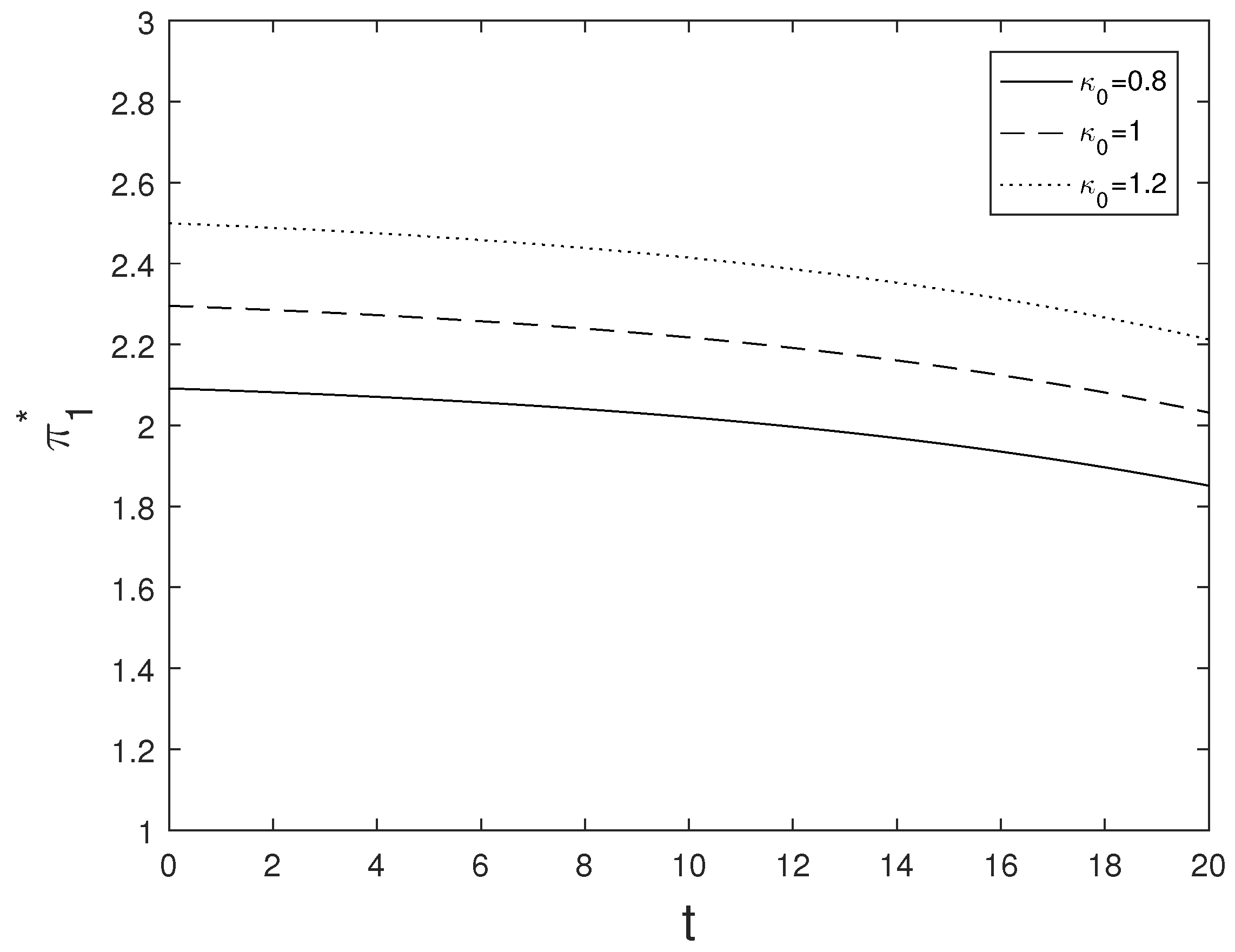
4.1. Optimal Investment Strategy

Figure 1 plots the impact of the risk-aversion coefficient $\gamma$ on optimal investment strategies ${\pi }_1^{*}$ and ${\pi }_2^{*}$. It is observed that as $\gamma$ increases, the optimal investment strategies ${\pi }_1^{*}$ and ${\pi }_2^{*}$ both decrease. The risk-aversion coefficient $\gamma$ increases, implying that the wage earner is more risk averse, and therefore accepts a lower investment risk. Thus, it is reasonable for investors with higher levels of risk aversion to adopt a more cautious investment strategy.

In Figure 2, the effect of the expected return rate $\lambda$ and volatility rate ${\sigma }_S$ on the optimal stock strategy ${\pi }_1^{*}$ is explored. Figure 2a shows that the optimal stock strategy ${\pi }_1^{*}$ increases as the expected rate of return $\lambda$ increases. However, as shown in Figure 2b, when the value of the volatility rate ${\sigma }_S$ increases, the optimal stock strategy ${\pi }_1^{*}$ decreases. It is common sense that as the expected rate of return $\lambda$ increases, investors will gain more from the stock market. However, an increase in instantaneous volatility ${\sigma }_S$ will lead to an increase in investment risk. Thus, as returns increase and volatility decreases, wage earners will invest more in risky assets, which is consistent with the general conclusion of the investment problem.

The impact of the expected inflation rate ${\lambda }_I$ and price-index volatility rate ${\sigma }_I$ on the optimal inflation-indexed bond strategy ${\pi }_2^{*}$ is shown in Figure 3. What can be seen is that the optimal bond strategy ${\pi }_2^{*}$ is larger when expected inflation ${\lambda }_I$ is larger and price index volatility ${\sigma }_I$ is lower. This observation implies that the wage earner stands to invest in the inflation-index bond if the expected inflation rate is higher and volatility is lower. This is because larger expected inflation implies larger inflation-indexed expected returns, while increased volatility in price indices implies increased uncertainty in investing in inflation-indexed bonds.

The effect of inside information on the optimal stock strategy ${\pi }_1^{*}$ is shown in Figure 4. According to Equation (2), the average rate at which the wage earner obtains inside information is captured by the parameter ${\kappa }_0$. We can observe that the optimal stock strategy ${\pi }_1^{*}$ is an increasing function of ${\kappa }_0$. This is a reasonable result from the assumption that the wage earner has a priori knowledge of the random variable $\mathcal{L}=B_S\left(T_0\right),T_0>T$ and $\kappa \left(t\right)$ is the drift induced by this random variable. This implies that the wage earner is taking advantage of additional information as an insider, and having access to inside stock information will encourage the wage earner to be bolder when investing in stocks. Moreover, since the inside information in our model only affects the stock process and not the inflation-index bond process, it is also quite natural that the optimal percentage invested in the inflation-index bond is not affected by the information drift.

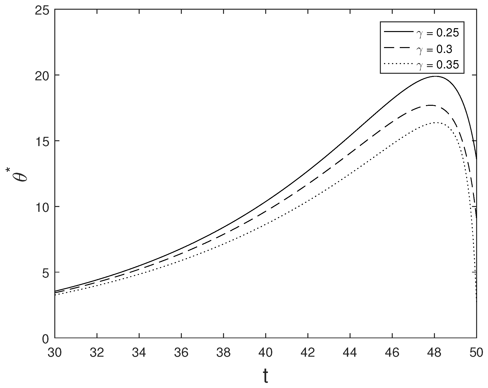
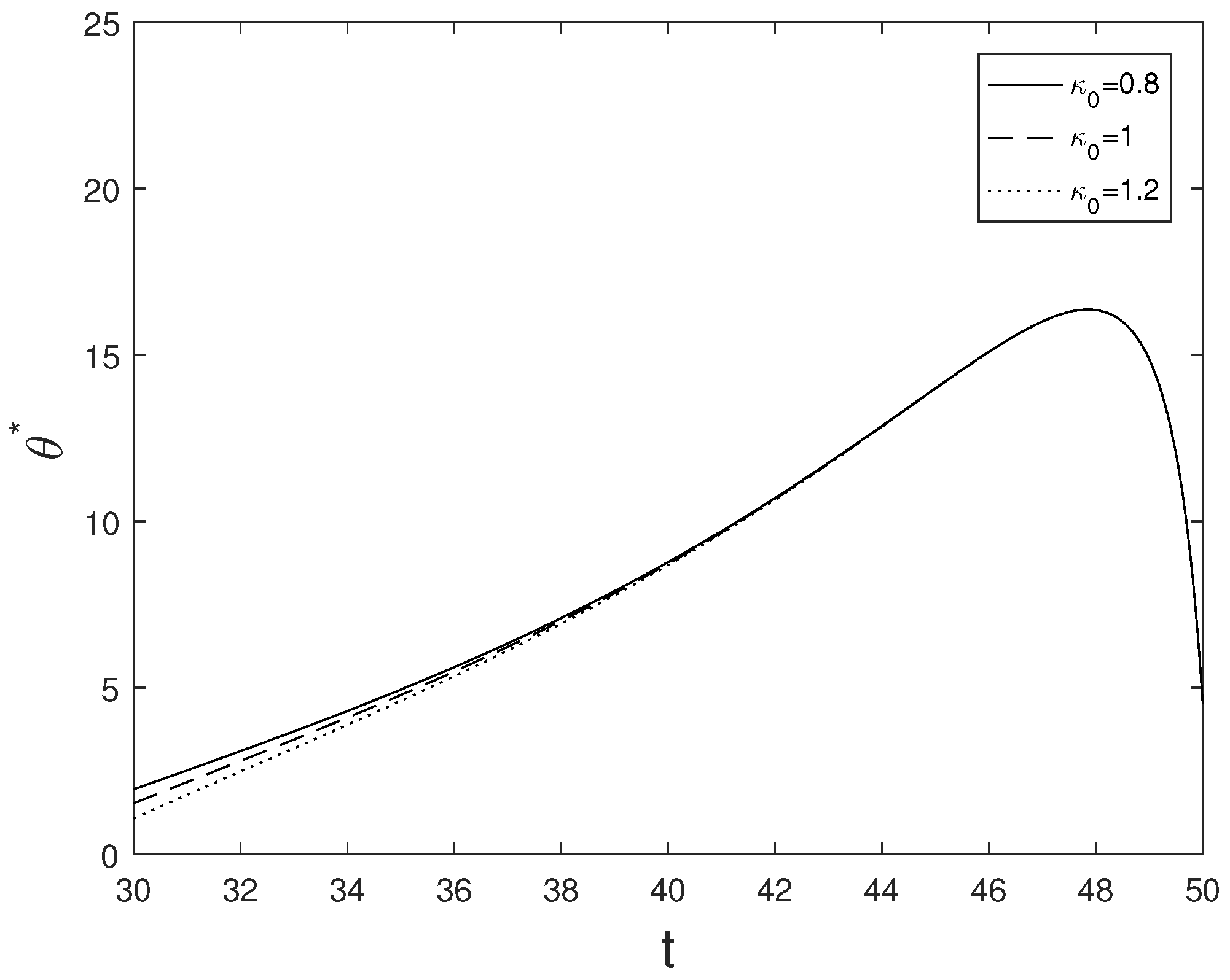
4.2. Optimal Life Insurance Strategy

In Figure 5, the influence of the risk-aversion coefficient $\gamma$ on the optimal life-insurance strategy ${\theta }^{*}$ is illustrated. As depicted in the graph, the spending on buying life insurance increases as $\gamma$ increases, indicating that the wage earner is inclined to purchase life insurance at an optimal level when he/she is more risk averse. Moreover, it shows that the optimal life-insurance strategy ${\theta }^{*}$ increases over time t before decreasing. This is because the risk of death increases as the wage earner gets older; thus, naturally, life-insurance purchases will increase. However, after a certain age, the wage earner has a higher mortality rate and it would cost more to purchase life insurance at this time. Combined with the fact that they may have accumulated some wealth, it is more cost-effective to take other economic actions than to purchase life insurance.

Figure 6 shows the impact of inside information on the optimal life-insurance strategy ${\theta }^{*}$. As the image illustrates, a higher value of ${\kappa }_0$ is associated with a larger optimal life-insurance strategy ${\theta }^{*}$. This may be because when more inside information about the stock is available, the wage earner is more certain about investing in stock and thus is more inclined to invest in risky markets to gain wealth. Therefore, the increase in investment and expected increase in wealth makes the wage earner less inclined to purchase life insurance to protect against financial risk.

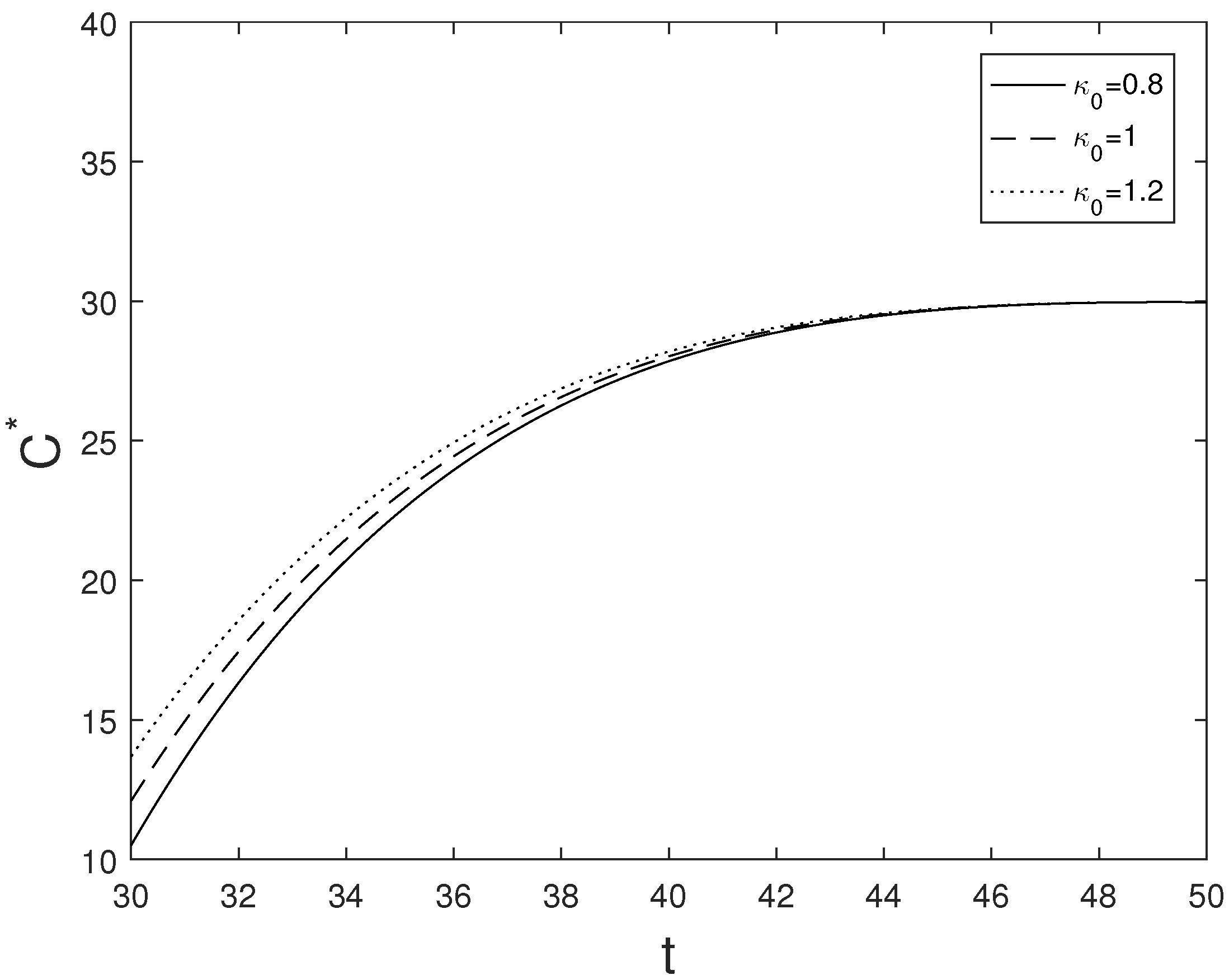
4.3. Optimal Consumption Strategy

Figure 7 plots the influence of the risk-aversion parameter $\gamma$ on the optimal consumption strategy $C^{*}$. The graph shows that as the value of the risk-aversion coefficient $\gamma$ rises, the optimal consumption strategy $C^{*}$ declines. This indicates that the higher the risk aversion of the wage earner, the more cautious the consumption, which is consistent with common sense.

Figure 8 shows the effect of inside information on optimal consumption strategy $C^{*}$. As can be seen, the larger the value of ${\kappa }_0$, the larger the corresponding optimal consumption strategy $C^{*}$. This implies that inside information about the stock will have a positive effect on the optimal consumption. This can be interpreted as follows: when the wage earner has more inside information about stock, he/she is more inclined to invest in risky assets; thus, an increase in wealth is expected. As a result, wage earners tend to spend more on consumption at the optimal level.

5. Conclusions

Due to the wide range of applications of life insurance in reality and the fact that it has become a current research hotspot, the factors influencing a wage earner’s investment, consumption and demand for life insurance under certain conditions need to be studied and justified. The economics of wage earners’ behavior under these conditions, including investment, consumption and life-insurance purchases also need to be analyzed. In this paper, we study the dynamically optimal consumption, investment and life-insurance strategies for a wage earner in the presence of inside information and inflation. Specifically, the dynamically optimal strategies for consumption, investment in risky assets, investment in inflation-indexed bonds and life insurance are obtained by maximizing the expected utility of consumption, inheritance and final wealth. To provide a comprehensive analysis, we consider alternative scenarios as well, including an inflation-free model and a model without the presence of inside information. Finally, in order to study the factors affecting the investment, consumption and life-insurance demand of the wage earner under conditions of inside information and inflation, sensitivity analysis is provided through numerical studies. The dynamically optimal strategies and value function properties suggest that the dynamic financial behavior of the wage earner are as follows: (i) Inside information leads to an increase in investment and consumption but a decrease in life-insurance purchases. (ii) As expected inflation increases and volatility decreases, the purchase of inflation-indexed bonds should be increased to protect against inflation risk. (iii) If wage earners are more risk-averse, they will invest more money in life insurance while reducing consumption and spending on investments in risky markets.

However, due to the complexity of life insurance as a product, the reality of life insurance is susceptible to a number of factors, such as the economic situation, the health status of the wage earner, the status of family members and the wage earner’s own subjective awareness of life insurance. The measurement of these real-world factors requires more sophisticated modeling to represent them. Therefore, the model in this paper explores more from a mathematical perspective, which has some limitations for the real situation. Consequently, more realistic models about investment, consumption and life insurance are expected.

References

1. Merton, R.C. Lifetime Portfolio Selection under Uncertainty: The Continuous-Time Case. Rev. Econ. Stat. 1969, 51, 247–257. [Google Scholar] [CrossRef] [Green Version]
2. Karatzas, I.; Lehoczky, J.P.; Sethi, S.P.; Shreve, S.E. Explicit solution of a general consumption/investment problem. Math. Oper. Res. 1986, 11, 261–294. [Google Scholar] [CrossRef]
3. Fleming, W.H.; Pang, T. An application of stochastic control theory to financial economics. Siam J. Control Optim. 2004, 43, 502–531. [Google Scholar] [CrossRef] [Green Version]
4. Chang, H.; Chang, K. Optimal consumption-investment strategy under the Vasicek model: HARA utility and Legendre transform. Insur. Math. Econ. 2017, 72, 215–227. [Google Scholar] [CrossRef]
5. Campbell, R.A. The Demand for Life Insurance: An Application of the Economics of Uncertainty. J. Financ. 1980, 35, 1155–1172. [Google Scholar] [CrossRef]
6. Richard, S.F. Optimal consumption, portfolio and life insurance rules for an uncertain lived individual in a continuous time model. J. Financ. Econ. 1975, 2, 187–203. [Google Scholar] [CrossRef]
7. Pliska, S.R.; Ye, J. Optimal life-insurance purchase and consumption/investment under uncertain lifetime. J. Bank. Financ. 2007, 31, 1307–1319. [Google Scholar] [CrossRef]
8. Huang, H.; Milevsky, M.A. Portfolio choice and mortality-contingent claims: The general HARA case. J. Bank. Financ. 2008, 32, 2444–2452. [Google Scholar] [CrossRef]
9. Pirvu, T.A.; Zhang, H. Optimal investment, consumption and life insurance under mean-reverting returns: The complete market solution. Insur. Math. Econ. 2012, 51, 303–309. [Google Scholar] [CrossRef]
10. Zeng, X.; Carsonb, J.M.; Chen, Q.; Wang, Y. Optimal life insurance with noborrowing constraints: Duality approach and example. Scand. Actuar. J. 2015, 9, 793–816. [Google Scholar]
11. Wei, J.; Cheng, X.; Jin, Z.; Wang, H. Optimal consumption–investment and life-insurance purchase strategy for couples with correlated lifetimes. Insur. Math. Econ. 2020, 91, 244–256. [Google Scholar] [CrossRef]
12. Wang, N.; Jin, Z.; Siu, T.K.; Qiu, M. Household consumption-investment-insurance decisions with uncertain income and market ambiguity. Scand. Actuar. J. 2021, 10, 832–865. [Google Scholar] [CrossRef]
13. Mousa, A.S.; Pinheiro, D.; Pinto, A.A. Optimal life-insurance selection and purchase within a market of several life-insurance providers. Insur. Math. Econ. 2016, 67, 133–141. [Google Scholar] [CrossRef] [Green Version]
14. Hoshiea, M.; Mousa, A.S.; Pinto, A.A. Optimal social welfare policy within financial and life insurance markets. Optimization 2022. [Google Scholar] [CrossRef]
15. Mousa, A.S.; Pinheiro, D.; Pinheiro, S.; Pinto, A.A. Optimal consumption, investment and life-insurance purchase under a stochastically fluctuating economy. Optimization 2022, 2022, 1–41. [Google Scholar] [CrossRef]
16. Kwak, M.; Lim, B.H. Optimal portfolio selection with life insurance under inflation risk. J. Bank. Financ. 2014, 46, 59–71. [Google Scholar] [CrossRef]
17. Han, N.W.; Hung, M.W. Optimal consumption, portfolio and life insurance policies under interest rate and inflation risks. Insur. Math. Econ. 2017, 73, 54–67. [Google Scholar] [CrossRef]
18. Liang, Z.; Zhao, X. Optimal mean-variance efficiency of a family with life insurance under inflation risk. Insur. Math. Econ. 2016, 71, 164–178. [Google Scholar] [CrossRef]
19. Shi, A.; Li, X.; Li, Z. Optimal investment, consumption and life insurance choices with habit formation and inflation risk. Complexity 2022, 2022, e3440037. [Google Scholar] [CrossRef]
20. Kyle, A. Continuous Auctions and Insider Trading. Econometrica 1985, 53, 1315–1335. [Google Scholar] [CrossRef] [Green Version]
21. Pikovsky, I.; Karatzas, I. Anticipative portfolio optimization. Adv. Appl. Probab. 1996, 28, 1095–1122. [Google Scholar] [CrossRef]
22. Imkeller, P.; Pontier, M.; Weisz, F. Free lunch and arbitrage possibilities in a financial market with an insider. Stoch. Process. Their Appl. 2001, 92, 103–130. [Google Scholar] [CrossRef] [Green Version]
23. Baltas, I.D.; Frangos, N.E.; Yannacopoulos, A.N. Optimal investment and reinsurance policies in insurance markets under the effect of inside information. Appl. Stoch. Model. Bus. Ind. 2012, 8, 506–528. [Google Scholar] [CrossRef]
24. Cao, J.; Peng, X.; Hu, Y. Optimal time-consistent investment and reinsurance strategy for mean-variance insurers under the inside information. Acta Math. Appl. Sin. 2016, 32, 1087–1100. [Google Scholar] [CrossRef]
25. Peng, X.; Wang, W. Optimal investment and risk control for an insurer under inside information. Insur. Math. Econ. 2016, 69, 104–116. [Google Scholar] [CrossRef]
26. Peng, X.; Chen, F.; Wang, W. Robust optimal investment and reinsurance for an insurer with inside information. Insur. Math. Econ. 2021, 96, 15–30. [Google Scholar] [CrossRef]
27. Peng, X.; Chen, F. Mean-variance asset-liability management with inside information. Commun. Stat.—Theory Methods 2022, 51, 2281–2302. [Google Scholar] [CrossRef]
28. Fleming, W.H.; Soner, H.M. Controlled Markov Processes and Viscosity Solutions, 2nd ed.; Springer: New York, NY, USA, 2006. [Google Scholar]
29. Ye, J. Optimal Life Insurance Purchase, Consumption and Portfolio under an Uncertain Life. Ph.D. Thesis, University of Illinois at Chicago, Chicago, IL, USA, 2006. [Google Scholar]
Figure 1. The effect of the risk-aversion parameter on the optimal investment strategies. (a) The effect of the risk-aversion parameter γ on the optimal stock strategy π 1 * . (b) The effect of the risk-aversion parameter γ on the optimal bond strategy π 2 * .
Mathematics 11 03415 g001
Figure 2. The effect of the expected return rate and volatility rate on the optimal stock strategy π 1 * . (a) The effect of the expected return rate λ on the optimal stock strategy π 1 * . (b) The effect of the volatility rate σ S on the optimal stock strategy π 1 * .
Mathematics 11 03415 g002
Figure 3. The effect of the expected inflation rate and volatility rate of price index on the optimal bond strategy π 2 * . (a) The effect of the expected inflation rate λ I of price index on the optimal bond strategy. (b) The effect of the volatility rate σ I of price index on the optimal bond strategy π 2 * .
Mathematics 11 03415 g003
Figure 4. The effect of the inside information on the optimal stock strategy π 1 * .
Mathematics 11 03415 g004
Figure 5. The effect of the risk-aversion parameter γ on the optimal life-insurance strategy θ * .
Mathematics 11 03415 g005
Figure 6. The effect of the inside information on the optimal life-insurance strategy θ * .
Mathematics 11 03415 g006
Figure 7. The effect of the risk-aversion parameter γ on the optimal consumption strategy C * .
Mathematics 11 03415 g007
Figure 8. The effect of inside information on the optimal consumption strategy C * .
Mathematics 11 03415 g008
Disclaimer/Publisher’s Note: The statements, opinions and data contained in all publications are solely those of the individual author(s) and contributor(s) and not of MDPI and/or the editor(s). MDPI and/or the editor(s) disclaim responsibility for any injury to people or property resulting from any ideas, methods, instructions or products referred to in the content.