Calculation Method and Application of Time-Varying Transmission Rate via Data-Driven Approach

Abstract

Most research about compartmental models of infection disease often consider the transmission rate as a constant, which is not ideal for the dynamic surveillance of infectious diseases. This study fully utilized continuously updated real-time epidemiological data and proposed a SEAIUHR model incorporating asymptomatic and symptomatic infectiousness, reported and unreported cases, inpatient and non-inpatient cases, and vaccine inoculation. This study proposed a novel approach based on our model to calculate the time-varying transmission rate with an under-report rate, vaccination efficiency, and relaxation of social distancing behavior. The proposed method was evaluated based on epidemiological data from the United States. The results suggest that using this approach to combine epidemiological data can provide a clearer understanding of the spread rule of epidemic, offering data support for subsequent related research.

1. Introduction

Mathematical modeling has been extensively used in many different fields of study including medicine, physics, economics, and so on [1,2,3,4,5,6,7,8,9,10,11,12,13,14,15,16,17,18,19,20]. Medical research issues, especially high-level medical research achievements, often rely on the establishment of reasonable medical mathematical models [7,8,9,10,11,12,13,14,15,16,17,18,19,20]. For example, Tripathi et al. [7] provided several examples of designing various mathematical models that can help us better comprehend dynamics at the single-cell and population levels. Gupta et al. [8] proposed a dynamic Boolean network to categorize gene regulation between two non-coding RNAs (ncRNAs) in gastric cancer, which opens up a new avenue for gastric cancer treatment in response to DNA damage caused by these ncRNAs. Lee et al. [9] utilized Bayesian inference and simulation to determine the relative contribution of each spatial structure and used it to generate hypotheses concerning the drivers of disease. The results demonstrated that Bayesian hierarchical models performed at least as well as existing modeling frameworks while permitting extensions in the future and multiple sources of spatial connectedness.

Furthermore, a compartment model of infectious diseases is crucial in understanding and controlling the transmission dynamics of infectious diseases, helping identify their epidemiological trends, making overall predictions, and offering interventions. The established model with the use of new epidemiological data can provide theoretical support for the prevention and control of infectious diseases, expose the mechanism of transmission, and facilitate the development of national and even international health policies [10]. After the outbreak of infectious diseases such as Ebola, COVID-19, and Plague, several domestic and foreign scholars refined the existing infectious disease models in use to analyze their epidemiological characteristics [11,12,13,14,15,16,17,18,19,20]. For example, a study [11] used two modified susceptible-infected-removed (SIR) models to simulate the transmission dynamics of Ebola, and the results showed that although there are currently no specific drugs to treat Ebola, effective isolation measures can better manage and control its transmission. Another study [13] improved the conventional susceptible-exposed-infected-removed (SEIR) model by incorporating four populations including people, rodents, fleas, and environmental pathogens in order to study the dynamics of Plague. The findings demonstrated that the spread of Plague to humans and rodents largely depends on the infected flea population.

As is well known, suitable models and reliable data are necessary to ascertain the spread mechanism of emerging infectious diseases, and a key point in establishing compartmental models of infection disease is to determine epidemiological characteristics. Though a large number of works, such as [11,12,13,14,15,16,17,18,19,20] and the references therein, have made it possible to research on the development of these disease with the previous models quantitatively or qualitatively, there still remains some uncertainties in the theoretical framework. To assure a vaccine’s efficacy and safety, it typically takes 10 to 15 years to produce one to combat emerging infectious diseases. However, for a few infectious diseases, the duration for vaccine research and development has greatly decreased. The most noticeable of these quick developments is vaccine efficacy, which describes the strength of a vaccine’s preventative effect and may influence the alleviation effect of nations implementing vaccinations. In addition, this is especially important when there are, inevitably, some unreported cases in the population which are also contagious, or some mild patients cannot be admitted for treatment during large-scale outbreaks of diseases. A few scholars have conducted in-depth discussions around these aspects.

Further, it is essential to determine the transmission rate ($\tau$), which helps shed more light and understanding on the spread and control strategies of emerging and re-emerging infectious diseases [21]. The parameters of compartmental models, including the transmission rate, are often chosen based on individual decisions or assumptions. For example, certain infectious disease models may assume that $\tau$ remains as a constant [12,13,15,18,20,22,23,24] or a piecewise constant [25,26] over the whole epidemic. However, a dynamic transmission rate is more reasonable than a constant one. Several studies have provided a time-varying form of transmission rate [27,28,29,30]. For instance, in reference [27], the author hypothesized that social distancing behavior would change due to fear of death, proposing a dynamic transmission rate. Although the calculation of transmission rate in the above literature is limited, since it will not change with newly released real-time data once it has been determined and the transmission rate may change due to many factors, not only a fear of increased deaths, including various preventive measures and changes in social distancing behavior. Their study provides reference for our research.

In this study, we frame a model to understand the complex interactions between the time-varying transmission rate and the epidemiological data, including daily reported cases data and daily vaccination data. Daily vaccination data, although they are unrefined, provide a better understanding of the effect of vaccine inoculation. We quantified the impact of changes in social distance behavior, vaccine efficacy, and unreported rates on transmission rates, using the established mathematical model to infer time-varying transmission rates. Finally, it was applied by using epidemiological data from the United States and our model’s stability and sensitivity were analyzed by varying vaccine efficacy and analyzing the resulting effects.

The remainder of this study is organized as follows: the formulation process by which an epidemic compartmental model is detailed in Section 2.1 and the transformation of our model is presented in Section 2.2, while the method of calculating the time–transmission rate is described in Section 2.3. Section 3 presents the application for epidemiological time-series datasets. The main conclusions of the study are made in Section 4.

2. Materials and Methods

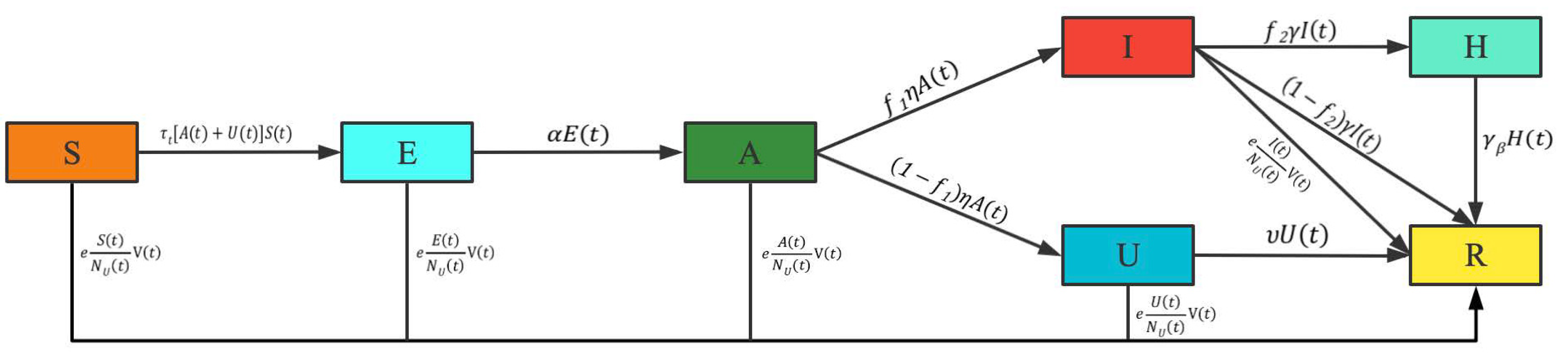
2.1. Epidemic Model

Our model is a system of ordinary differential equations for the epidemic population compartments and we divide the population into seven compartments: susceptible individuals (S), exposed individuals (E), asymptomatic infectious individuals (A), reported symptomatic infectious individuals (I), under-reported symptomatic infectious individuals (U), hospitalized individuals (H), and recovered individuals (R). The following reasonable assumptions are made to simplify the problem.

Hypothesis 1. 

$S\left(t\right),E\left(t\right),A\left(t\right),I\left(t\right),U\left(t\right),H\left(t\right),$ and $R\left(t\right)$ denote, at time t, the number of the seven population categories, S, E, A, I, U, H, and R, respectively.

Hypothesis 2. 

It is well known that not all cases are reported by government agencies. There inevitably exist some undocumented infections in the population due to some uncontrollable reasons. We define this type of population as U. Reported symptomatic infectious individuals are isolated immediately, and cause no further infections. However, A and U are infectious; thus, S may be infected by them. Assuming the transmission rate is ${\tau }_t$, at time t, the increment content of E equals ${\tau }_t[A\left(t\right)+U\left(t\right)]S\left(t\right)$.

Hypothesis 3. 

E has been infected but is not yet capable of propagating the infection. Assuming average duration of the exposed period is $\frac{1}{\alpha }$, at time t, the increment content of A equals $\alpha E\left(t\right)$.

Hypothesis 4. 

Assuming that a symptomatic infection can only be converted through A, the average duration of the asymptomatic infectious period is $\frac{1}{\eta }$, and the report rate of symptomatic infectious individuals is $f_1$, so at time t, the increment content of I and U equal $f_1\eta A\left(t\right)$ and $(1-f_1)\eta A\left(t\right)$, respectively.

Hypothesis 5. 

Assuming that average duration of a reported symptomatic infectious period is $\frac{1}{\gamma }$, the hospitalization rate is $f_2$, so at time t, the increment content of H equals $f_2\gamma I\left(t\right)$.

Hypothesis 6. 

$V\left(t\right)$ is the daily number of vaccinated individuals, and $N_U\left(t\right)$ is the number of unvaccinated individuals. So, $\frac{S\left(t\right)}{N_U\left(t\right)},\frac{E\left(t\right)}{N_U\left(t\right)},\frac{A\left(t\right)}{N_U\left(t\right)},\frac{I\left(t\right)}{N_U\left(t\right)},$ and $\frac{U\left(t\right)}{N_U\left(t\right)},$ denote, at time t, the fraction of S, E, A, I, and U in the unvaccinated individuals, respectively. Assuming that vaccine efficacy is e, at time t, the number of S, E, A, I, and U who have recovered due to vaccination equal $e\frac{S\left(t\right)}{N_U\left(t\right)}V\left(t\right),e\frac{E\left(t\right)}{N_U\left(t\right)}V\left(t\right),e\frac{A\left(t\right)}{N_U\left(t\right)}V\left(t\right),e\frac{I\left(t\right)}{N_U\left(t\right)}V\left(t\right),$ and $e\frac{U\left(t\right)}{N_U\left(t\right)}V\left(t\right)$.

Hypothesis 7. 

Assuming that the average duration of an unreported symptomatic infectious period and hospitalized period are $\frac{1}{\upsilon }$ and $\frac{1}{{\gamma }_{\beta }}$, respectively, at time t, the increment content of R equals ${\gamma }_{\beta }H\left(t\right)+(1-f_2)\gamma I\left(t\right)+\upsilon U\left(t\right)+e\frac{S\left(t\right)+E\left(t\right)+A\left(t\right)+I\left(t\right)+U\left(t\right)}{N_U\left(t\right)}V\left(t\right)$.

Under the above hypotheses, the diagram for the model is shown in Figure 1.

The SEAIUHR model is governed by the following nonautonomous ordinary differential equations

$$\left\{\begin{array}{cc}\hfill S^{\prime }\left(t\right)& =-{\tau }_t[A\left(t\right)+U\left(t\right)]S\left(t\right)-e\frac{S\left(t\right)}{N_U\left(t\right)}V\left(t\right),\hfill \\ \hfill E^{\prime }\left(t\right)& ={\tau }_t[A\left(t\right)+U\left(t\right)]S\left(t\right)-\alpha E\left(t\right)-e\frac{E\left(t\right)}{N_U\left(t\right)}V\left(t\right),\hfill \\ \hfill A^{\prime }\left(t\right)& =\alpha E\left(t\right)-\eta A\left(t\right)-e\frac{A\left(t\right)}{N_U\left(t\right)}V\left(t\right),\hfill \\ \hfill I^{\prime }\left(t\right)& =f_1\eta A\left(t\right)-\gamma I\left(t\right)-e\frac{I\left(t\right)}{N_U\left(t\right)}V\left(t\right),\hfill \\ \hfill U^{\prime }\left(t\right)& =(1-f_1)\eta A\left(t\right)-\upsilon U\left(t\right)-e\frac{U\left(t\right)}{N_U\left(t\right)}V\left(t\right),\hfill \\ \hfill H^{\prime }\left(t\right)& =f_2\gamma I\left(t\right)-{\gamma }_{\beta }H\left(t\right),\hfill \\ \hfill R^{\prime }\left(t\right)& ={\gamma }_{\beta }H\left(t\right)+(1-f_2)\gamma I\left(t\right)+\upsilon U\left(t\right)+e\frac{S\left(t\right)+E\left(t\right)+A\left(t\right)+I\left(t\right)+U\left(t\right)}{N_U\left(t\right)}V\left(t\right).\hfill \end{array}\right.$$

(1)

Due to the fact that no individuals were vaccinated at the beginning of the infectious disease (i.e., $t=t_0$), the total population N at $t_0$ is

$$N=S_0+E_0+A_0+I_0+U_0+H_0,$$

The total number of vaccinated individuals from $t_1$ to $t_2$ ($t_2>t_1$) is

$${\int }_{t_1}^{t_2}V\left(s\right)ds,$$

The cumulative number of vaccinated individuals is

$$CV\left(t\right)={\int }_{t_0}^{t}V\left(s\right)ds,$$

So

$$C{V}^{\prime }\left(t\right)=V\left(t\right),$$

(2)

The number of unvaccinated individuals is

$$N_U\left(t\right)=N-CV\left(t\right).$$

(3)

The state variables H and R are decupled from the rest of model (1), so we will not focus on their dynamic in the following. Then, using (2) and (3), model (1) is transformed into

$$\left\{\begin{array}{cc}\hfill S^{\prime }\left(t\right)& =-{\tau }_t[A\left(t\right)+U\left(t\right)]S\left(t\right)-e\frac{S\left(t\right)}{N-CV\left(t\right)}C{V}^{\prime }\left(t\right),\hfill \\ \hfill E^{\prime }\left(t\right)& ={\tau }_t[A\left(t\right)+U\left(t\right)]S\left(t\right)-\alpha E\left(t\right)-e\frac{E\left(t\right)}{N-CV\left(t\right)}C{V}^{\prime }\left(t\right),\hfill \\ \hfill A^{\prime }\left(t\right)& =\alpha E\left(t\right)-\eta A\left(t\right)-e\frac{A\left(t\right)}{N-CV\left(t\right)}C{V}^{\prime }\left(t\right),\hfill \\ \hfill I^{\prime }\left(t\right)& =f_1\eta A\left(t\right)-\gamma I\left(t\right)-e\frac{I\left(t\right)}{N-CV\left(t\right)}C{V}^{\prime }\left(t\right),\hfill \\ \hfill U^{\prime }\left(t\right)& =(1-f_1)\eta A\left(t\right)-\upsilon U\left(t\right)-e\frac{U\left(t\right)}{N-CV\left(t\right)}C{V}^{\prime }\left(t\right).\hfill \end{array}\right.$$

(4)

The number of the cumulative reported cases grows exponentially approximately with time, evolving at the early stage [26]. The cumulative reported confirmed cases at time t, denoted by $CI\left(t\right)$, are formatted as follows:

$$CI\left(t\right)=aexp\left(bt\right)-c,t\ge t_0.$$

(5)

The parameters $a,b$, and c are to be determined by the least squares estimation method. It is obvious that the cumulative reported confirmed data are zero at $t_0$. Then, we obtain

$$t_0=\frac{1}{b}ln\frac{c}{a}.$$

(6)

2.2. Transformation of the System (4)

In order to frame a model which can be easily tractable, a few simplifying conversions are in order. The simplifying method can contribute to our model, making it possible to calculate the time-varying transmission rate that will offer data support for subsequent related research.

Set

$$\psi \left(t\right):=exp(e{\int }_{t_0}^t\frac{-C{V}^{\prime }\left(s\right)}{N-CV\left(s\right)}ds),$$

then,

$$\psi \left(t\right)=(\frac{N-CV\left(t\right)}{N-CV\left(t_0\right)}).$$

(7)

By integrating the first equation of system (4), we obtain

$$S\left(t\right)=S_{0}exp\left\{-{\int }_{t_0}^t{\tau }_s[A\left(s\right)+U\left(s\right)]ds+(e{\int }_{t_0}^t\frac{-C{V}^{\prime }\left(s\right)}{N-CV\left(s\right)}ds)\right\},$$

Therefore, we obtain

$$S\left(t\right)=S_{0}exp\left\{-{\int }_{t_0}^t{\tau }_s[A\left(s\right)+U\left(s\right)]ds\right\}\psi \left(t\right).$$

(8)

By setting

$$\overline{S}\left(t\right):=\frac{S\left(t\right)}{\psi \left(t\right)},$$

we have

$${\overline{S}}^{\prime }\left(t\right)=-{\tau }_t[A\left(t\right)+U\left(t\right)]\overline{S}\left(t\right).$$

Define

$$\overline{E}\left(t\right):=\frac{E\left(t\right)}{\psi \left(t\right)},$$

so we have

$${\overline{E}}^{\prime }\left(t\right)=\frac{E^{\prime }\left(t\right)}{\psi \left(t\right)}+e\frac{E\left(t\right)}{N-CV\left(t\right)}\frac{C{V}^{\prime }\left(t\right)}{\psi \left(t\right)}.$$

(9)

Substituting (8) into the second equation of system (4), we obtain

$$E^{\prime }\left(t\right)={\tau }_t[A\left(t\right)+U\left(t\right)]S_{0}exp\left\{-{\int }_{t_0}^t{\tau }_s[A\left(s\right)+U\left(s\right)]ds\right\}\psi \left(t\right)-\alpha E\left(t\right)-e\frac{E\left(t\right)}{N-CV\left(t\right)}C{V}^{\prime }\left(t\right).$$

(10)

Substituting (10) into (9), we obtain

$${\overline{E}}^{\prime }\left(t\right)={\tau }_t[A\left(t\right)+U\left(t\right)]\overline{S}\left(t\right)-\alpha \overline{E}\left(t\right).$$

For the same reason, define

$$\overline{A}\left(t\right):=\frac{A\left(t\right)}{\psi \left(t\right)},\overline{I}\left(t\right):=\frac{I\left(t\right)}{\psi \left(t\right)},\overline{U}\left(t\right):=\frac{U\left(t\right)}{\psi \left(t\right)}.$$

By using the same method for the remaining equations of system (4), we obtain

$${\overline{A}}^{\prime }\left(t\right)=\alpha \overline{E}\left(t\right)-\eta \overline{A}\left(t\right),$$

$${\overline{I}}^{\prime }\left(t\right)=f_1\eta \overline{A}\left(t\right)-\gamma \overline{I}\left(t\right),$$

$${\overline{U}}^{\prime }\left(t\right)=(1-f_1)\eta \overline{A}\left(t\right)-\upsilon \overline{U}\left(t\right).$$

Thus, system (4) is transformed as follows:

$$\left\{\begin{array}{cc}\hfill {\overline{S}}^{\prime }\left(t\right)& =-{\tau }_t[A\left(t\right)+U\left(t\right)]\overline{S}\left(t\right),\hfill \\ \hfill {\overline{E}}^{\prime }\left(t\right)& ={\tau }_t[A\left(t\right)+U\left(t\right)]\overline{S}\left(t\right)-\alpha \overline{E}\left(t\right),\hfill \\ \hfill {\overline{A}}^{\prime }\left(t\right)& =\alpha \overline{E}\left(t\right)-\eta \overline{A}\left(t\right),\hfill \\ \hfill {\overline{I}}^{\prime }\left(t\right)& =f_1\eta \overline{A}\left(t\right)-\gamma \overline{I}\left(t\right),\hfill \\ \hfill {\overline{U}}^{\prime }\left(t\right)& =(1-f_1)\eta \overline{A}\left(t\right)-\upsilon \overline{U}\left(t\right).\hfill \end{array}\right.$$

(11)

and

$$\overline{S}\left(t_0\right)=S\left(t_0\right),\overline{E}\left(t_0\right)=E\left(t_0\right),\overline{A}\left(t_0\right)=A\left(t_0\right),\overline{I}\left(t_0\right)=I\left(t_0\right),\overline{U}\left(t_0\right)=U\left(t_0\right).$$

2.3. Method of Calculating the Time-Varying Transmission Rate

In reality, a dynamic $\tau$ could be adequate to capture the course of an epidemic. Our goal is to apply the transformed system (11) to calculate the time-varying transmission rate using daily reported cases data and daily vaccination data. Daily reported cases are extremely erratic; hence, we use a 7-day moving average to smooth these data and use $\psi \left(t\right)$ for normalization. Let $d\overline{i}\left(t_1\right),d\overline{i}\left(t_2\right),d\overline{i}\left(t_3\right),\dots$, be the 7-day moving average of daily reported cases normalized by $\psi \left(t\right)$, where $t_1,t_2,t_3,\dots$, are discrete variables. And we use the least squares method to discretize these discrete data. The continuous version of $d\overline{i}\left(t_1\right),d\overline{i}\left(t_2\right),d\overline{i}\left(t_3\right),\dots$, denoted by $D\overline{I}\left(t\right)$, is formatted as follows

$$D{\overline{I}}^{\prime }\left(t\right)=f_1\eta \overline{A}\left(t\right)-D\overline{I}\left(t\right).$$

hence, $A\left(t\right)$ normalized by $\psi \left(t\right)$ to satisfy

$$\overline{A}\left(t\right)=\frac{D{\overline{I}}^{\prime }\left(t\right)+D\overline{I}\left(t\right)}{f_1\eta }.$$

(12)

Substituting (12) into the third equation of system (11), we obtain

$$\overline{E}\left(t\right)=\frac{D{\overline{I}}^{″}\left(t\right)+(\eta +1)D{\overline{I}}^{\prime }\left(t\right)+\eta D\overline{I}\left(t\right)}{\alpha f_1\eta }.$$

(13)

Substituting (13) into the second equation of system (11), we obtain

$${\tau }_t=\frac{[D{\overline{I}}^{‴}\left(t\right)+(\alpha +\eta +1)D{\overline{I}}^{″}\left(t\right)+(\alpha \eta +\eta +\alpha )D{\overline{I}}^{\prime }\left(t\right)+\alpha \eta D\overline{I}\left(t\right)]}{\alpha f_1\eta \overline{S}\left(t\right)(A\left(t\right)+U\left(t\right))}.$$

(14)

We assume that $\frac{I\left(t\right)}{U\left(t\right)}=\frac{f_1}{1-f_1}$ and $A\left(t\right)=\frac{D{\overline{I}}^{\prime }\left(t\right)+D\overline{I}\left(t\right)}{f_1\eta }\psi \left(t\right)$ in terms of (12). Therefore, the time-varying transmission rate before social distancing behavior relaxation is formatted as follows

$${\tau }_t=\frac{f_1[D{\overline{I}}^{‴}\left(t\right)+(\alpha +\eta +1)D{\overline{I}}^{″}\left(t\right)+(\alpha \eta +\eta +\alpha )D{\overline{I}}^{\prime }\left(t\right)+\alpha \eta D\overline{I}\left(t\right)]}{\alpha \overline{S}\left(t\right)[(D{\overline{I}}^{\prime }\left(t\right)+D\overline{I}\left(t\right))\psi \left(t\right)f_1+(1-f_1)I\left(t\right)]}.$$

(15)

According to the common rule of disease development, there is an increasing return to normal of social distancing behavior in most cases. Therefore, we introduce a social behavior relaxation parameter $\delta$ (i.e., degree of relaxation) to quantify the impact of increasing return of social distancing behavior on time-varying transmission. After a period of relaxation, there is no further change, in social distance. Therefore, the subsequent transmission rate is divided into two stages, namely $t_1\le t\le t_2$ and $t\ge t_2$, where $t_1$ and $t_2$ correspond to the day before the change in social distance and the time of no further change in social distance, respectively. In this study, we suggest that the probability of asymptomatic infected individuals and unreported symptomatic infected individuals transmitting to susceptible individuals is the same, but $A\left(t\right),U\left(t\right),$ and $S\left(t\right)$ vary as time evolves. We calculate the subsequent time-varying transmission rate including $\delta ,A\left(t\right),U\left(t\right)$, and $S\left(t\right)$ based on ${\tau }_{t_1}$.

For $t_1\le t\le t_2$, the transmission rate is formatted as follows:

$${\tau }_t={\tau }_{t_1}[1+\delta (t-t_1)]\frac{\left(A\right(t)+U(t\left)\right)S\left(t\right)}{(A\left(t_1\right)+U\left(t_1\right))S\left(t_1\right)}.$$

(16)

For $t\ge t_2$, the transmission rate is formatted as follows:

$${\tau }_t={\tau }_{t_1}[1+\delta (t_2-t_1)]\frac{\left(A\right(t)+U(t\left)\right)S\left(t\right)}{(A\left(t_1\right)+U\left(t_1\right))S\left(t_1\right)}.$$

(17)

3. Application

3.1. Data Preparation

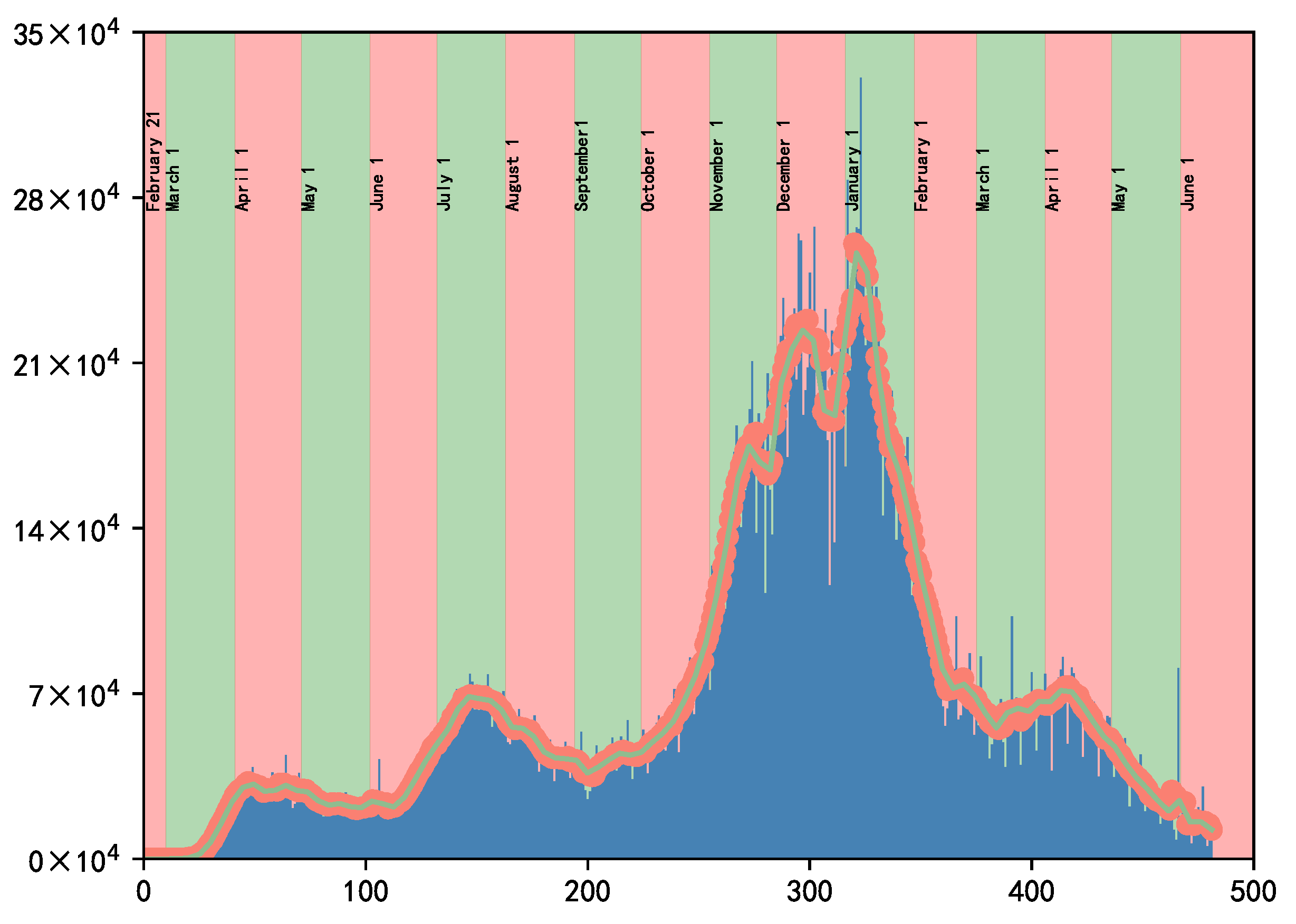
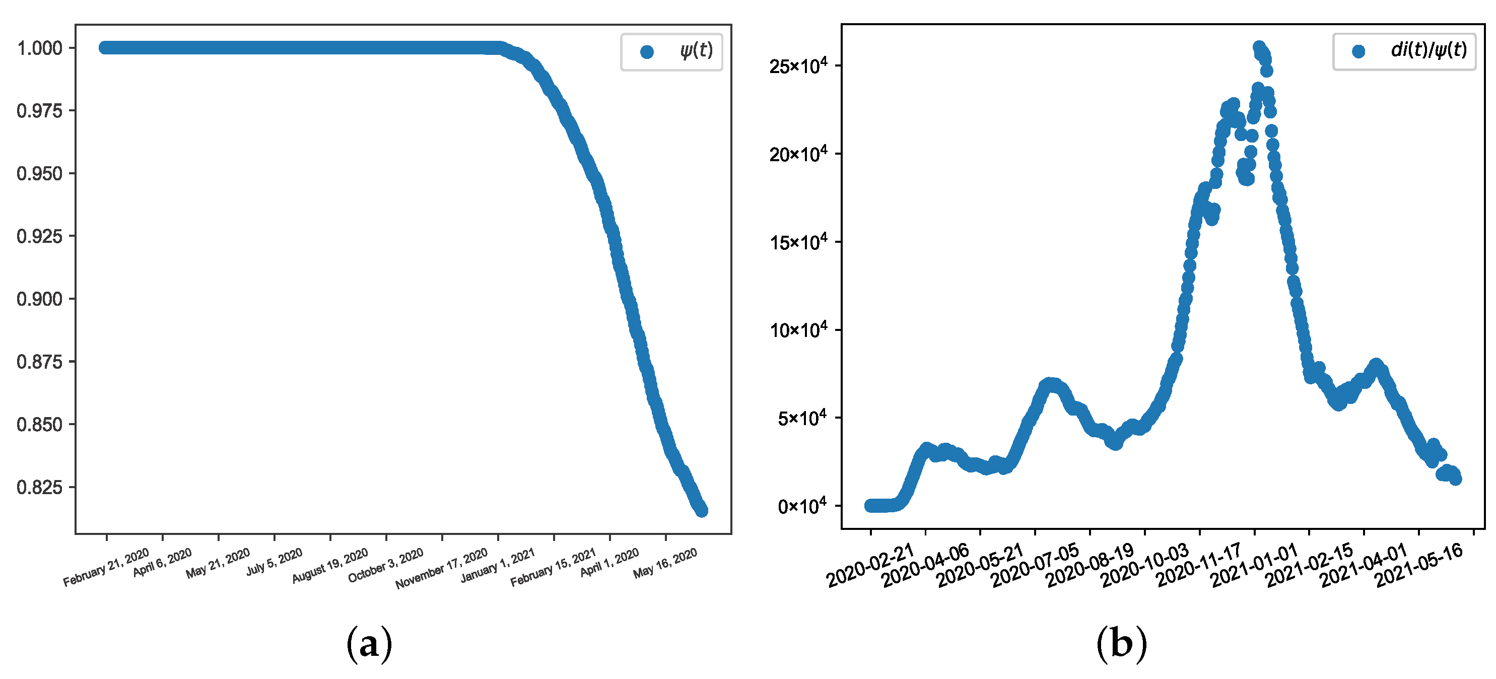
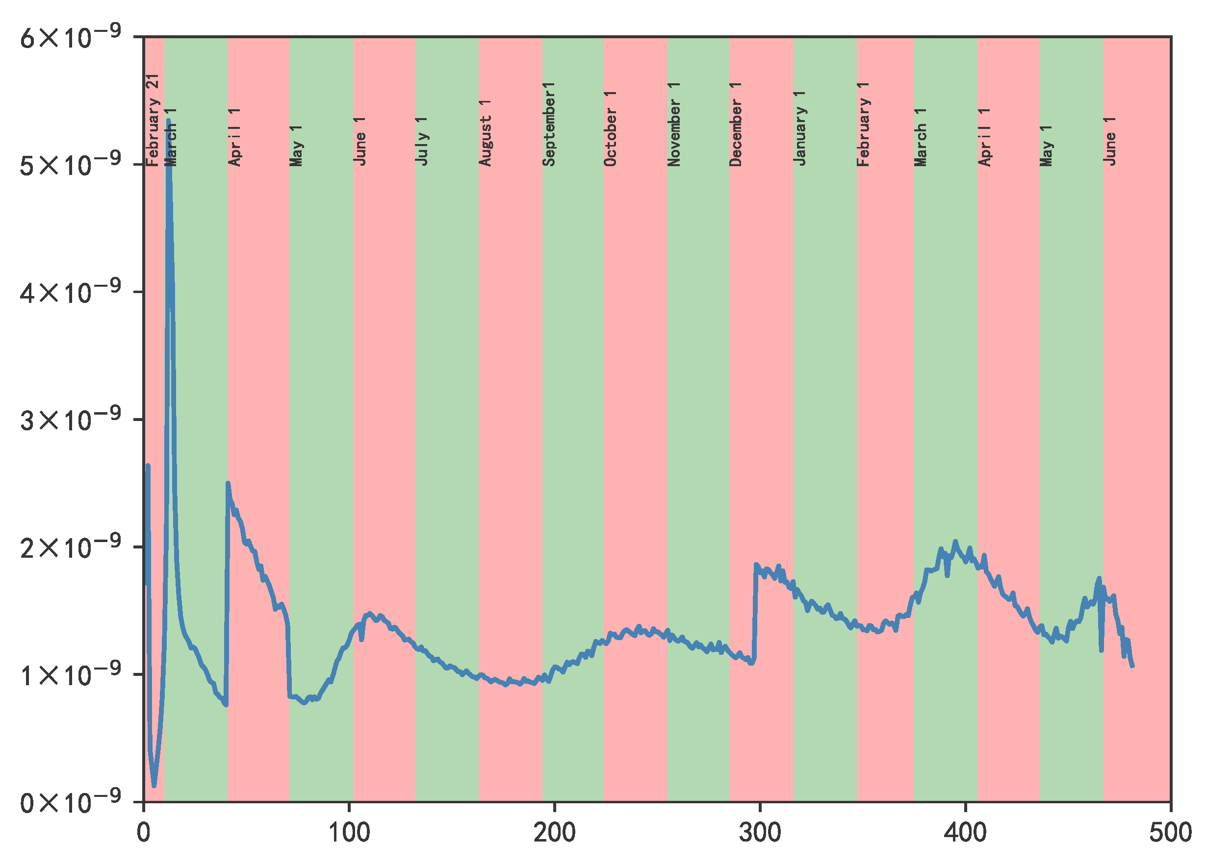
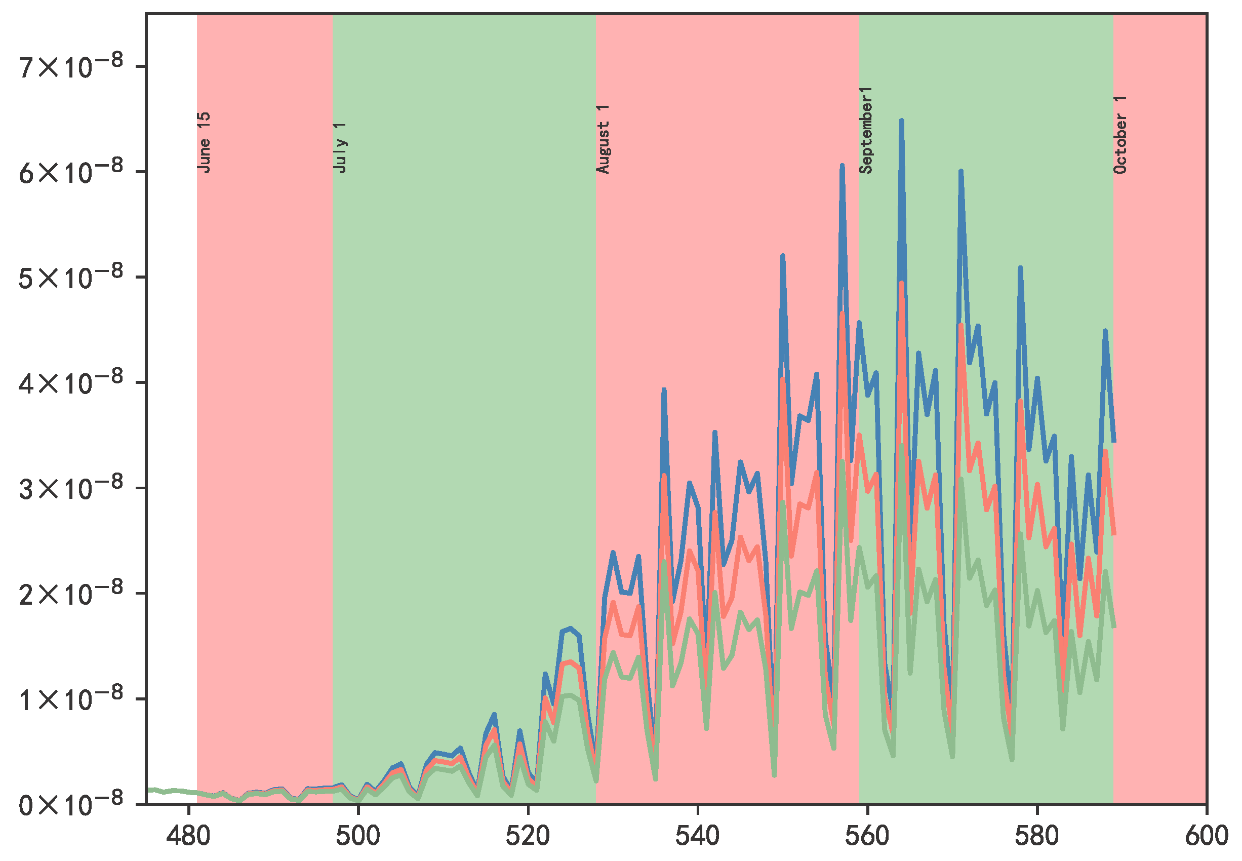
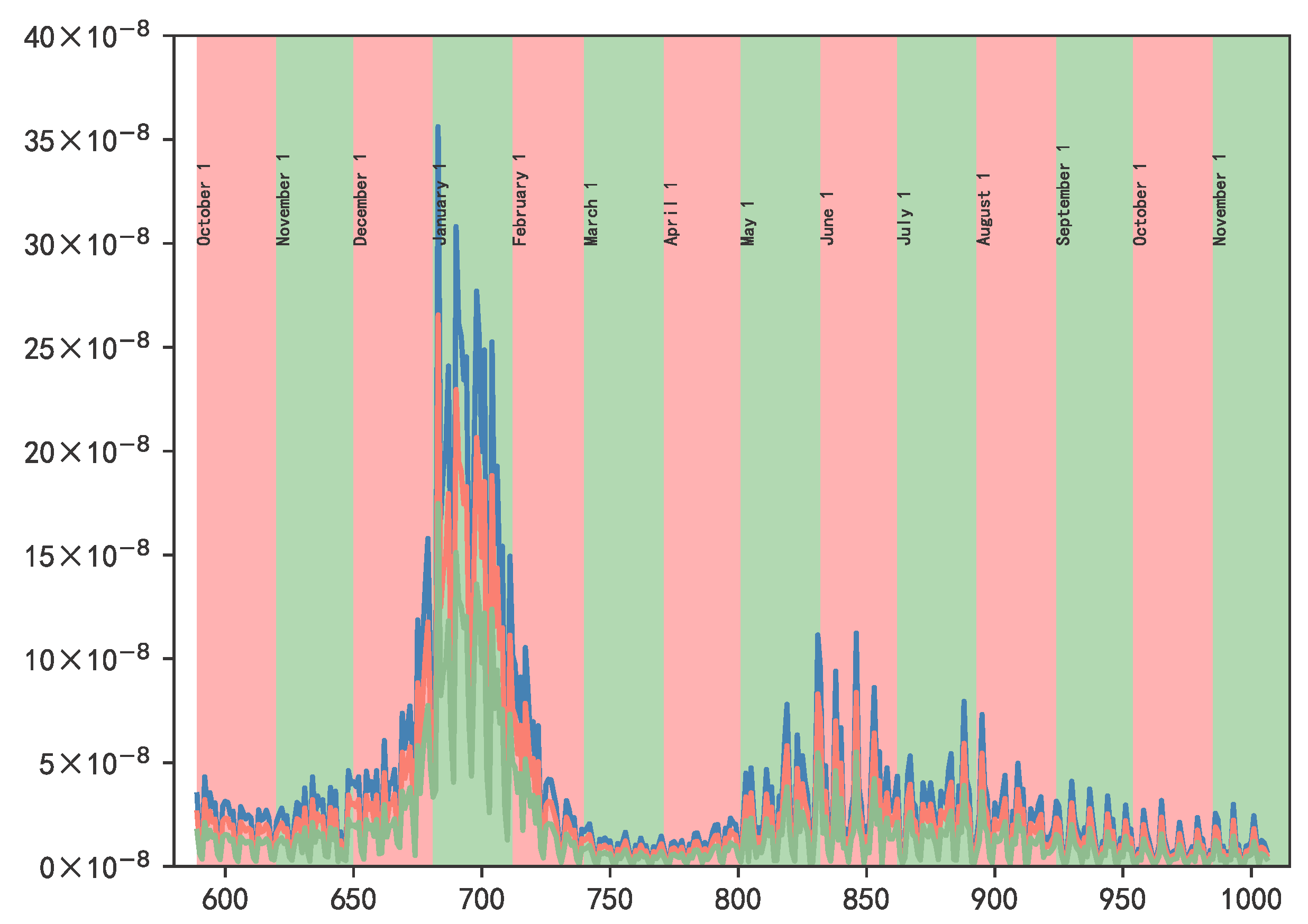
This study used Formulas (15)–(17) to simulate epidemiological time-series datasets in the United States. Furthermore, daily reported cases data, daily vaccination data, and demographic data were obtained from the Center for Systems Science and Engineering at Johns Hopkins University [31], the Centers for Disease Control and Prevention [32], and the US Census Bureau [33], respectively.

3.2. Results

Firstly, using the cumulative confirmed cases as shown in

Table 1. The cumulative data of confirmed cases.

Data	03/08	03/09	03/10	03/11	03/12	03/13	03/14	03/15	03/16
Cases	213	472	696	987	1264	1678	2995	3782	4661

, we fixed the value of parameter c as 1, and then estimated the values of parameters $a=14.57$ and $b=0.37$ using the least squares method. According to Equation (6), we calculated $t_0=-7.24$, which corresponds to 21 February 2020. From 15 June 2021 to 1 October 2021, social distancing behavior gradually returned. After 1 October 2021, there was no further change in social distancing behavior. Therefore, $t_1$, and $t_2$ correspond to 15 June 2021 and 1 October 2021, respectively.

It can be seen, from Formulas (15)–(17), that the selection of susceptible individuals and parameter values is essential for calculating time-varying transmission rate. Parameter values are exhibited in

Table 2. Parameter values of system (11).

Parameter	Value	Source
N	331,108,434	[33]
e	$0.63$	[34]
$f_1$	$\frac{5}{17}$	[35]
$\frac{1}{\alpha }$	3	[36]
$\frac{1}{\eta }$	5	[37]
$\frac{1}{\upsilon }$	7	[38]

. According to the chronology in the US, we set the number of susceptible individuals as: (1) $S\left(t\right)=N$ from 21 February 2020 to 31 March 2020; (2) $S\left(t\right)=\frac{3}{10}N$ from 1 April 2020 to 30 April 2020; (3) $S\left(t\right)=\frac{1}{2}N$ from 1 May 2020 to 13 December 2020; and (4) $S\left(t\right)=\frac{3}{10}N$ after 14 December 2020.

In Figure 2, the blue vertical bars are the daily reported cases from $t_0$ to $t_1$, the red dots are the 7-day moving average of daily reported cases, and the green graph is the continuum cubic spline interpolation of red dots. Shown in Figure 3a, we plotted $\psi \left(t\right)$ from $t_0$ to $t_1$, and the daily number of reported cases was normalized using $\psi \left(t\right)$ (i.e., $d\overline{i}\left(t\right)$), as shown in Figure 3b.

By using parameters values as shown in Table 2 and Formula (15), the time-varying transmission rate from $t_0$ to $t_1$ can be determined, which was graphed and is shown in Figure 4. It can be seen that ${\tau }_{t_1}=1.06976518931823\times {10}^{-9}$, $S\left(t_1\right)=$ 99,332,530, $A\left(t_1\right)=$ 243,350, and $I\left(t_1\right)=$ 16,946, $U\left(t_1\right)=$ 40,670 from the model output, whereupon we calculated the time-varying transmission rates from $t_1$ to $t_2$ and after $t_2$ in terms of ${\tau }_{t_1},S\left(t_1\right),A\left(t_1\right),U\left(t_1\right)$, and Formulas (16) and (17), as presented in Figure 5 and Figure 6. The blue, red, and green lines correspond to the transmission rate of $\delta =0.03$, $\delta =0.02$, and $\delta =0.01$. In what follows, vaccine efficacy was set to 0, 0.63, and 1; the peaks of time-varying transmission rates at each stage and the time of occurrence are presented in

Table 3. Peak values of time-varying transmission rates and the time of occurrence at each stage ($e=0$).

		${\mathit{\tau }}_{\mathit{t}}$
		Time	Peak Value
First stage		3 March 2020	$5.34452\times {10}^{-9}$
Second stage	$\delta =0.01$		$4.51811\times {10}^{-8}$
	$\delta =0.02$	6 September 2021	$6.56731\times {10}^{-8}$
	$\delta =0.03$		$8.61651\times {10}^{-8}$
Third stage	$\delta =0.01$		$2.32183\times {10}^{-7}$
	$\delta =0.02$	3 January 2022	$3.52739\times {10}^{-7}$
	$\delta =0.03$		$4.73295\times {10}^{-7}$

,

Table 4. Peak values of time-varying transmission rates and the time of occurrence at each stage ($e=0.63$).

		${\mathit{\tau }}_{\mathit{t}}$
		Time	Peak Value
First stage		3 March 2020	$5.34379\times {10}^{-9}$
Second stage	$\delta =0.01$		$3.40048\times {10}^{-8}$
	$\delta =0.02$	6 September 2021	$4.94278\times {10}^{-8}$
	$\delta =0.03$		$6.48508\times {10}^{-8}$
Third stage	$\delta =0.01$		$1.74748\times {10}^{-7}$
	$\delta =0.02$	3 January 2022	$2.65483\times {10}^{-7}$
	$\delta =0.03$		$3.56218\times {10}^{-7}$

and

Table 5. Peak values of time-varying transmission rates and the time of occurrence at each stage ($e=1$).

		${\mathit{\tau }}_{\mathit{t}}$
		Time	Peak Value
First stage		3 March 2020	$5.34286\times {10}^{-9}$
Second stage	$\delta =0.01$		$3.15718\times {10}^{-8}$
	$\delta =0.02$	6 September 2021	$4.58912\times {10}^{-8}$
	$\delta =0.03$		$6.02107\times {10}^{-8}$
Third stage	$\delta =0.01$		$1.62245\times {10}^{-7}$
	$\delta =0.02$	3 January 2022	$2.46488\times {10}^{-7}$
	$\delta =0.03$		$3.30730\times {10}^{-7}$

, respectively. Meanwhile, $e=0$ means that the vaccine is completely ineffective, and $e=1$ means that the vaccine is completely effective.

Furthermore, conditional on Table 3, Table 4 and Table 5, we can obtain some conclusions. Due to vaccine inoculation beginning in the US on 14 December 2020, there is no significant difference in peak values of time-varying transmission rates for $e=0,0.63,1$ during the first stage. It can be seen that when the vaccine is not effective at all, the situation of peak value is much worse at the second and third stages. However, the circumstances are better when the vaccine is fully effective.

4. Conclusions

In the present study, we formulated a SEAIUHR compartment model that reflects the relationship between susceptible, exposed, asymptomatic, symptomatic, hospitalized, and recovered individuals under vaccination. By introducing $\psi \left(t\right)$, we transformed the SEAIUHR model into a model that can be easily tractable. We linked the model to factors that may lead to disease transmission including under-report rate, vaccination efficiency, and relaxation of social distancing behavior. A data-driven approach was adopted to calculate the time-varying transmission rate in terms of time series with daily reported cases data and daily vaccination data. The extremely erratic daily reported cases data were smoothed using the weekly moving average, and the least squares method was used to continuously process the discrete data. By using the cumulative confirmed cases, we concluded that the starting time for the compartments is $t_0$. The transmission rate after day $t_1$ is based on the model transmission rate on this day. We set two dates, $t_1$ and $t_2$, in terms of the reduction in social distancing measures, such that $t_1\le t\le t_2$ and $t\ge t_2$; the transmission rate changed with $A\left(t\right),U\left(t\right)$, and $S\left(t\right)$; and the social behavior relaxation parameter was $\delta$.

The designed method was applied to epidemiological time-series datasets in the United States. According to chronology and Formula (6), $t_0,t_1$, and $t_2$ correspond to 21 February 2020, 15 June 2021 and 1 October 1, 2021, respectively. The model outputs were analyzed with the under-report rate $(1-f_1)$ as $\frac{12}{17}$, vaccine efficacy $\left(e\right)$ as 0.63, and social behavior relaxation parameters $\delta =0.03,\delta =0.02$, and $\delta =0.01$. The model output shows the time-varying transmission rate of everyday. Meanwhile, we demonstrated the model’s stability and sensitivity to changes in input variables by varying the value of e and analyzing the resulting effects.

The method to calculate time-varying transmission rate via a data-driven approach, in comparison to a constant or a piecewise constant transmission rate, can capture the actual transmission dynamics and provide data support for subsequent research. When dealing with the emerging and re-emerging infectious diseases that may arise, the model compartments can be appropriately adjusted to adapt to varied epidemic characteristics, but the method of transmission rate of our research has high universality. High universality means that the calculation method proposed in our study can be applied to calculate the transmission rate of these diseases after determining the compartment model according to the characteristics of infectious diseases.

However, this study does have certain limitations. First, here we failed to consider immunized individuals and dead individuals. These could be added to our model, and other phenomena could be included as well, such as a fading rate of immunity by age class, provided the relevant parameters are known. Second, the majority of parameters change over time as the infectious disease progresses, but we fixed a few of them according to existing studies to reduce uncertainty. Each parameter value will need to be enhanced further in future research.

References

1. Michelsen, C. Mathematical modeling is also physics—Interdisciplinary teaching between mathematics and physics in Danish upper secondary education. Phys. Educ. 2015, 50, 489. [Google Scholar] [CrossRef]
2. Hsieh, K.T.; Rajamani, R.K. Mathematical model of the hydrocyclone based on physics of fluid flow. AIChE J. 1991, 37, 735–746. [Google Scholar] [CrossRef]
3. Johns, P.B. A new mathematical model to the physics of propagation. Radio Electron. Eng. 1974, 44, 657–666. [Google Scholar] [CrossRef]
4. Borodin, A.I.; Tatuev, A.A.; Shash, N.N.; Lyapuntsova, E.V.; Rokotyanskaya, V.V. Economic-mathematical model of building a company’s potential. Asian Soc. Sci. 2015, 11, 198. [Google Scholar] [CrossRef] [Green Version]
5. Shaimardanovich, D.A.; Rustamovich, U.S. Economic-mathematical modeling of optimization production of agricultural production. Asia Pac. J. Res. Bus. Manag. 2018, 9, 10–21. [Google Scholar]
6. Vovk, O.; Tulchynska, S.; Popelo, O.; Tulchinskiy, R.; Tkachenko, T. Economic and Mathematical Modeling of the Integration Impact of Modernization on Increasing the Enterprise Competitiveness. Manag. Theory Stud. Rural Bus. Infrastruct. Dev. 2021, 43, 383–389. [Google Scholar] [CrossRef]
7. Tripathi, S.; Xing, J.; Levine, H.; Jolly, M.K. Mathematical modeling of plasticity and heterogeneity in EMT. Methods Mol. Biol. 2021, 2179, 385–413. [Google Scholar]
8. Gupta, S.; Panda, P.K.; Luo, W.; Hashimoto, R.F.; Ahuja, R. Network analysis reveals that the tumor suppressor lncRNA GAS5 acts as a double-edged sword in response to DNA damage in gastric cancer. Sci. Rep. 2022, 12, 18312. [Google Scholar] [CrossRef]
9. Lee, S.A.; Economou, T.; Lowe, R. A Bayesian modelling framework to quantify multiple sources of spatial variation for disease mapping. J. R. Soc. Interface 2022, 19, 20220440. [Google Scholar] [CrossRef]
10. Heesterbeek, H.; Anderson, R.M.; Andreasen, V.; Bansal, S.; De Angelis, D.; Dye, C.; Eames, K.T.; Edmunds, W.J.; Frost, S.D.; Funk, S.; et al. Modeling infectious disease dynamics in the complex landscape of global health. Science 2015, 347, aaa4339. [Google Scholar] [CrossRef] [Green Version]
11. Osemwinyen, A.C.; Diakhaby, A. Mathematical modelling of the transmission dynamics of ebola virus. Appl. Comput. Math. 2015, 4, 313–320. [Google Scholar] [CrossRef]
12. Rachah, A. Analysis, simulation and optimal control of a SEIR model for Ebola virus with demographic effects. Commun. Fac. Sci. Univ. Ank. Ser. A1 Math. Stat. 2018, 67, 179–197. [Google Scholar]
13. Ngeleja, R.C.; Luboobi, L.S.; Nkansah-Gyekye, Y. Modelling the dynamics of bubonic plague with yersinia pestis in the environment. Commun. Math. Biol. Neurosci. 2016, 2016, 10. [Google Scholar]
14. Foley, J.E.; Zipser, J.; Chomel, B.; Girvetz, E.; Foley, P. Modeling plague persistence in host-vector communities in California. J. Wildl. Dis. 2007, 43, 408–424. [Google Scholar] [CrossRef] [Green Version]
15. Hidayati, N.; Sari, E.R.; Waryanto, N.H. Mathematical model of Cholera spread based on SIR: Optimal control. Pythagoras J. Pendidik. Mat. 2021, 16, 70–83. [Google Scholar] [CrossRef]
16. Fung, I.C.H. Cholera transmission dynamic models for public health practitioners. Emerg. Themes Epidemiol. 2014, 11, 1. [Google Scholar] [CrossRef] [Green Version]
17. Zakary, O.; Larrache, A.; Rachik, M.; Elmouki, I. Effect of awareness programs and travel-blocking operations in the control of HIV/AIDS outbreaks: A multi-domains SIR model. Adv. Differ. Equ. 2016, 2016, 169. [Google Scholar] [CrossRef] [Green Version]
18. Mwalili, S.; Kimathi, M.; Ojiambo, V.; Gathungu, D.; Mbogo, R. SEIR model for COVID-19 dynamics incorporating the environment and social distancing. BMC Res. Notes 2020, 13, 352. [Google Scholar] [CrossRef]
19. Cooper, I.; Mondal, A.; Antonopoulos, C.G. A SIR model assumption for the spread of COVID-19 in different communities. Chaos Solitons Fractals 2020, 139, 110057. [Google Scholar] [CrossRef]
20. Clark, D.E.; Welch, G.; Peck, J.S. A modified SIR model equivalent to a generalized logistic model, with standard logistic or log-logistic approximations. IISE Trans. Healthc. Syst. Eng. 2022, 12, 130–136. [Google Scholar] [CrossRef]
21. Jing, M.; Ng, K.Y.; Mac Namee, B.; Biglarbeigi, P.; Brisk, R.; Bond, R.; Finlay, D.; McLaughlin, J. COVID-19 modelling by time-varying transmission rate associated with mobility trend of driving via Apple Maps. J. Biomed. Inform. 2021, 122, 103905. [Google Scholar] [CrossRef] [PubMed]
22. Wintachai, P.; Prathom, K. Stability analysis of SEIR model related to efficiency of vaccines for COVID-19 situation. Heliyon 2021, 7, e06812. [Google Scholar] [CrossRef] [PubMed]
23. Ghostine, R.; Gharamti, M.; Hassrouny, S.; Hoteit, I. An extended SEIR model with vaccination for forecasting the COVID-19 pandemic in Saudi Arabia using an ensemble Kalman filter. Mathematics 2021, 9, 636. [Google Scholar] [CrossRef]
24. Capaldi, A.; Behrend, S.; Berman, B.; Smith, J.; Wright, J.; Lloyd, A.L. Parameter estimation and uncertainty quantication for an epidemic model. Math. Biosci. Eng. 2012, 553–576. [Google Scholar] [CrossRef]
25. Abdy, M.; Side, S.; Annas, S.; Nur, W.; Sanusi, W. An SIR epidemic model for COVID-19 spread with fuzzy parameter: The case of Indonesia. Adv. Differ. Equ. 2021, 2021, 105. [Google Scholar] [CrossRef]
26. Liu, Z.; Magal, P.; Webb, G. Predicting the number of reported and unreported cases for the COVID-19 epidemics in China, South Korea, Italy, France, Germany and United Kingdom. J. Theor. Biol 2021, 509, 110501. [Google Scholar] [CrossRef]
27. Fernández-Villaverde, J.; Jones, C.I. Estimating and simulating a SIRD model of COVID-19 for many countries, states, and cities. J. Econ. Dyn. Control 2022, 140, 104318. [Google Scholar] [CrossRef]
28. Chowell, G.; Hengartner, N.W.; Castillo-Chavez, C.; Fenimore, P.W.; Hyman, J.M. The basic reproductive number of Ebola and the effects of public health measures: The cases of Congo and Uganda. J. Theor. Biol. 2004, 229, 119–126. [Google Scholar] [CrossRef] [Green Version]
29. Chowell, G.; Viboud, C.; Hyman, J.M. The Western Africa ebola virus disease epidemic exhibits both global exponential and local polynomial growth rates. PLoS Curr. 2015, 7. [Google Scholar] [CrossRef]
30. Viboud, C.; Simonsen, L.; Chowell, G.; Simonsen, L. A generalized-growth model to characterize the early ascending phase of infectious disease outbreaks. Epidemics 2016, 15, 27–37. [Google Scholar] [CrossRef] [Green Version]
31. Johns Hopkins Coronavirus Resource Center. Available online: https://coronavirus.jhu.edu/map.html (accessed on 28 February 2023).
32. Centers for Disease Control and Prevention. Available online: https://covid.cdc.gov/covid-data-tracker/#vaccinations_vacc-people-booster-percent-total (accessed on 28 February 2023).
33. United States Census. Available online: https://ballotpedia.org/United_States_census,_2020#cite_note-1 (accessed on 6 March 2023).
34. Britton, A.; Slifka, K.M.J.; Edens, C.; Nanduri, S.A.; Bart, S.M.; Shang, N.; Harizaj, A.; Armstrong, J.; Xu, K.; Ehrlich, H.Y.; et al. Effectiveness of the Pfizer-BioNTech COVID-19 vaccine among residents of two skilled nursing facilities experiencing COVID-19 outbreaks—Connecticut, December 2020–February 2021. Morb. Mortal. Wkly. Rep. 2021, 70, 396. [Google Scholar] [CrossRef]
35. Centers for Disease Control and Prevention. Available online: https://www.cdc.gov/coronavirus/2019-ncov/cases-updates/burden.html (accessed on 6 March 2023).
36. Demongeot, J.; Griette, Q.; Magal, P.; Webb, G. Modeling vaccine efficacy for COVID-19 outbreak in New York city. Biology 2022, 11, 345. [Google Scholar] [CrossRef] [PubMed]
37. Li, Q.; Guan, X.; Wu, P.; Wang, X.; Zhou, L.; Tong, Y.; Ren, R.; Leung, K.S.M.; Lau, E.H.Y.; Wong, J.Y.; et al. Early transmission dynamics in Wuhan, China, of novel coronavirus—Infected pneumonia. N. Engl. J. Med. 2020, 382, 1199–1207. [Google Scholar] [CrossRef] [PubMed]
38. Xie, H.; Tao, J.; McHugo, G.J.; Drake, R.E. Comparing statistical methods for analyzing skewed longitudinal count data with many zeros: An example of smoking cessation. J. Subst. Abuse Treat. 2013, 45, 99–108. [Google Scholar] [CrossRef] [PubMed]
Figure 1. Schematic diagram of the model compartments: susceptible, exposed, asymptomatic infected, reported symptomatic infected, under-reported symptomatic infected, hospitalized, and recovered.
Mathematics 11 02955 g001
Figure 2. Diagram of daily reported cases, 7-day moving average of daily reported cases, and the continuum cubic spline interpolation of 7-day moving average of daily reported cases from 21 February 2020 to 15 June 2021.
Mathematics 11 02955 g002
Figure 3. In (a), we plot ψ ( t ) from 21 February 2020 to 15 June 2021. In (b), we plot d i ¯ ( t ) ψ ( t ) from 21 February 2020 to 15 June 2021.
Mathematics 11 02955 g003
Figure 4. Diagram of the time-varying transmission rate from 21 February 2020 to 15 June 2021.
Mathematics 11 02955 g004
Figure 5. Diagram of the time-varying transmission rate from 15 June 2021 to 1 October 2021, with δ = 0.03 , δ = 0.02 , and δ = 0.01 .
Mathematics 11 02955 g005
Figure 6. Diagram of the time-varying transmission rate from 1 October 2021 to 22 November 2022, with δ = 0.03 , δ = 0.02 , and δ = 0.01 .
Mathematics 11 02955 g006