
Rapid Estimation of Contact Stresses in Imageless Total Knee Arthroplasty

Abstract
:1. Introduction
2. Methodology
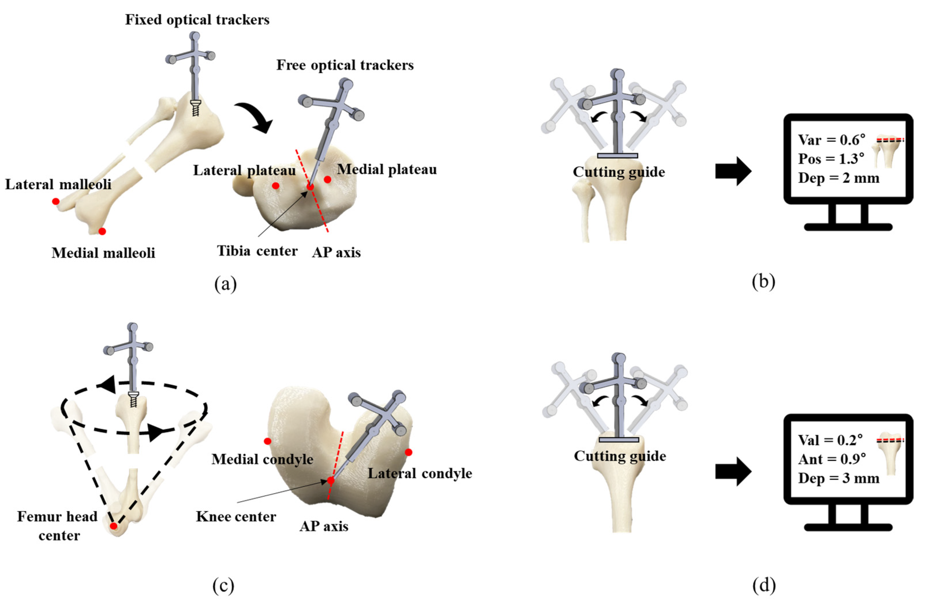
2.1. TKA Procedure
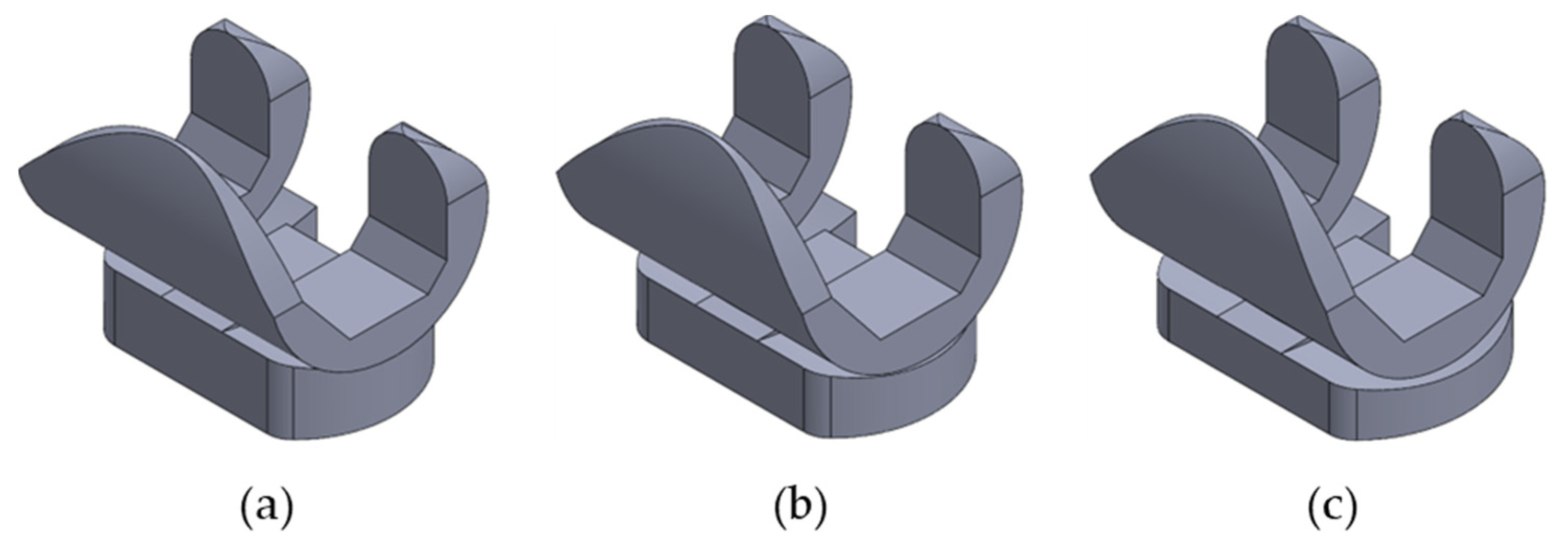
2.2. CAD Model Development
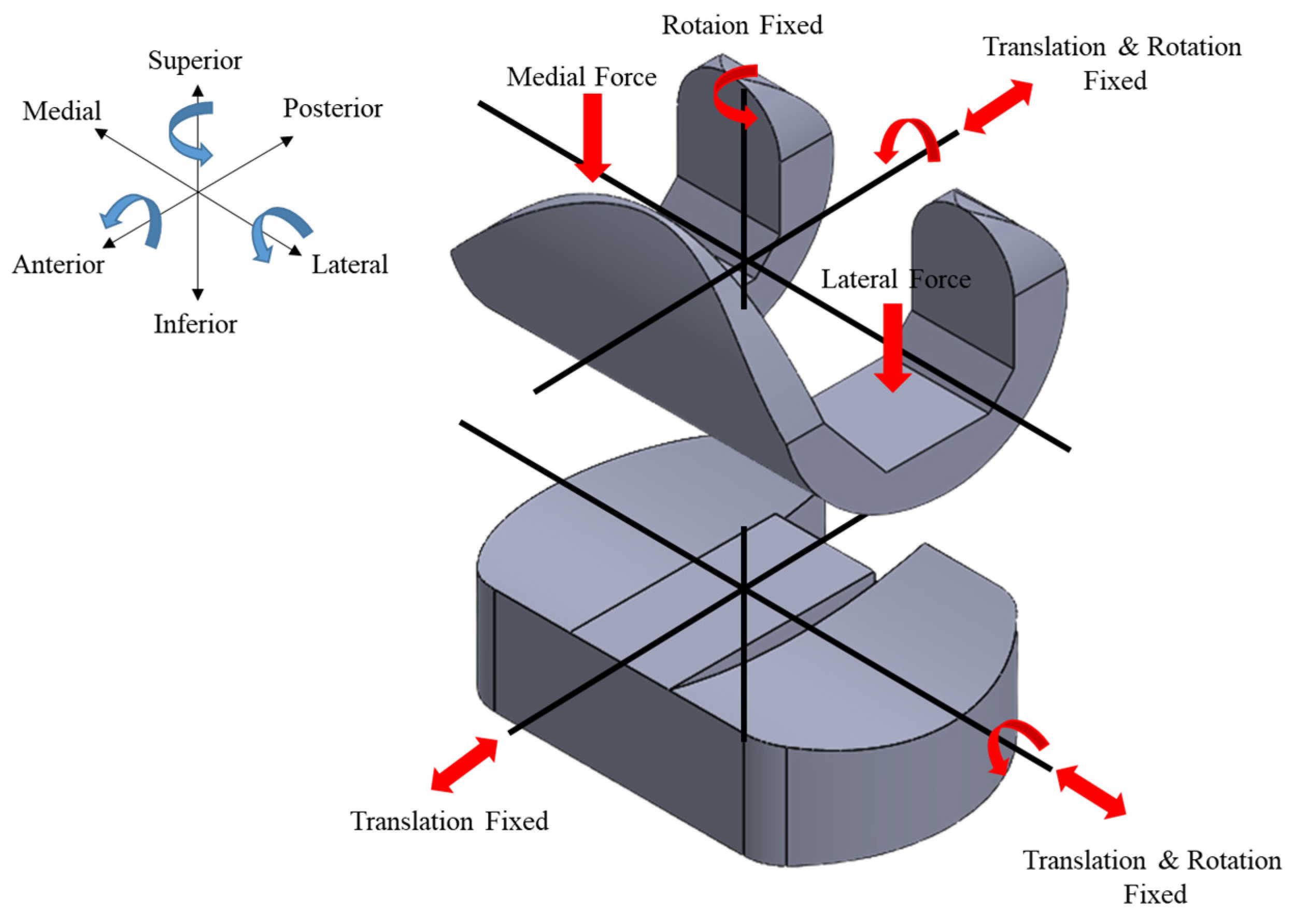
2.3. FEA Model Development
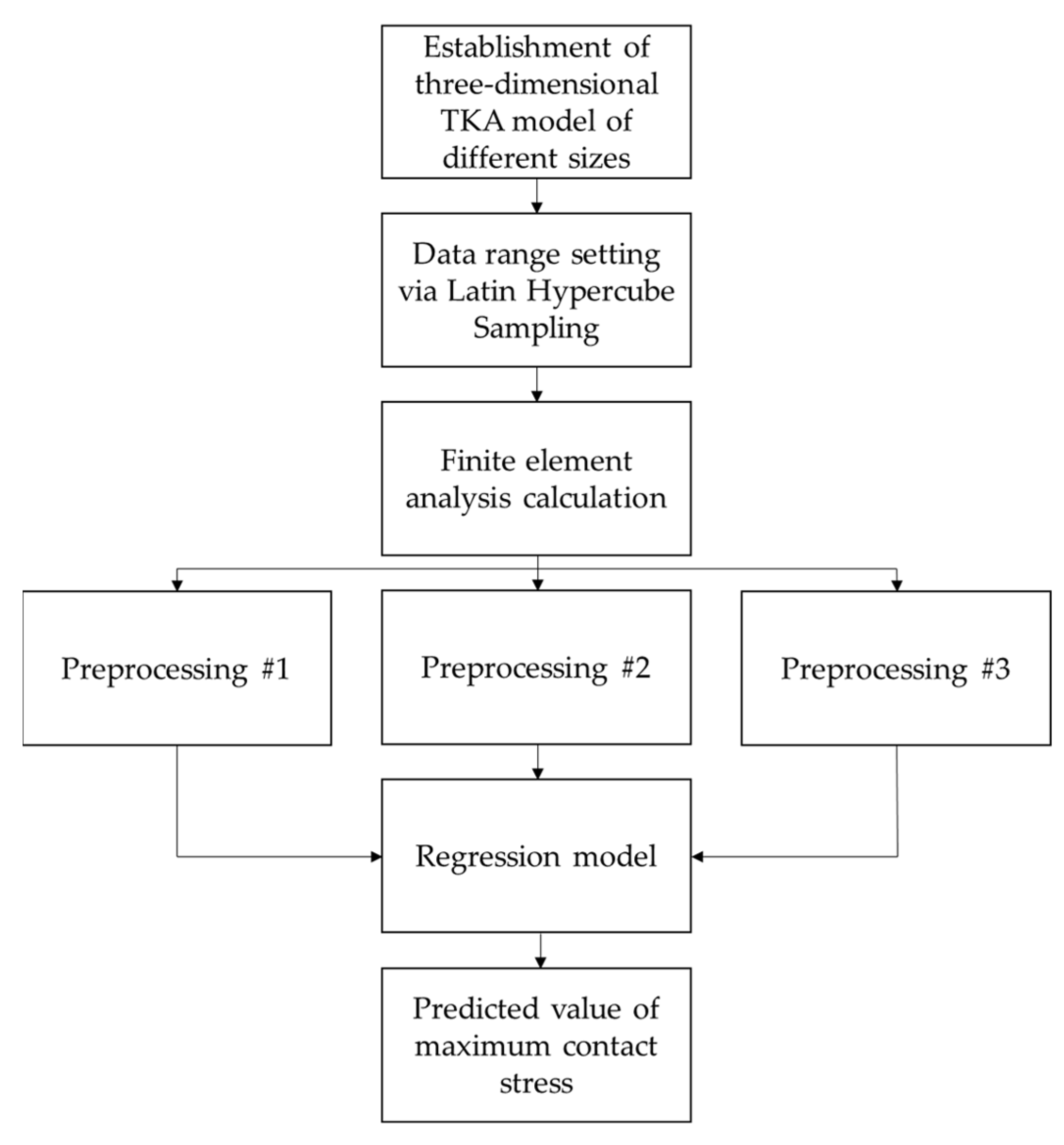
2.4. Prediction Model Development
3. Results and Discussion
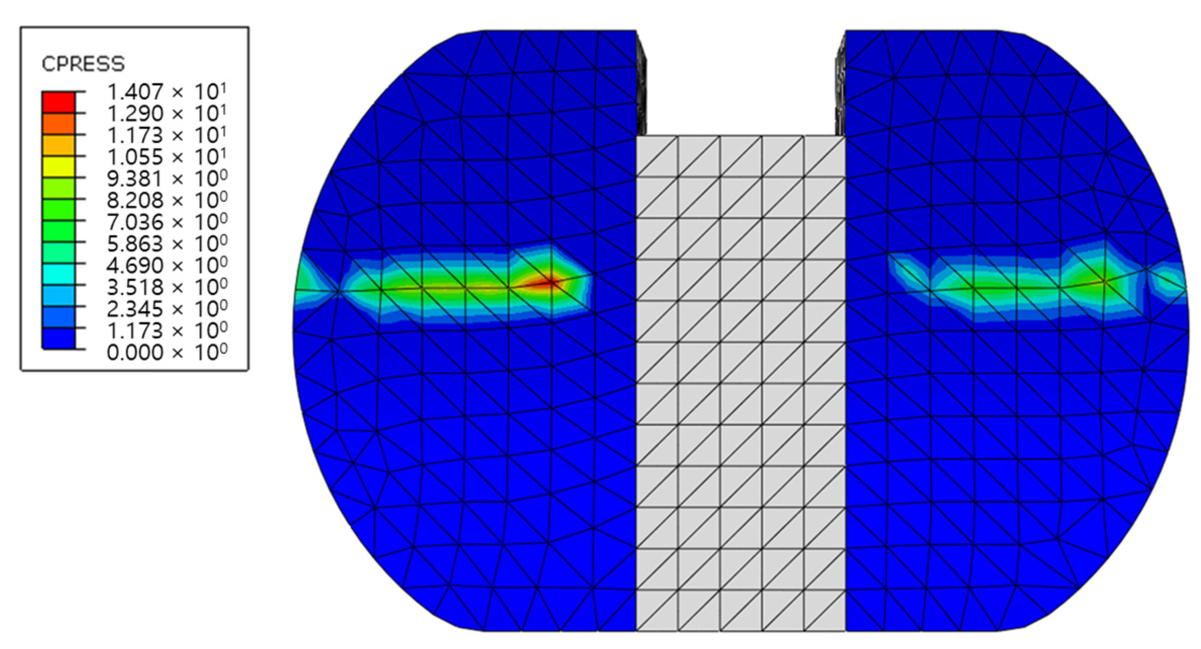
3.1. Validation of FEM Model
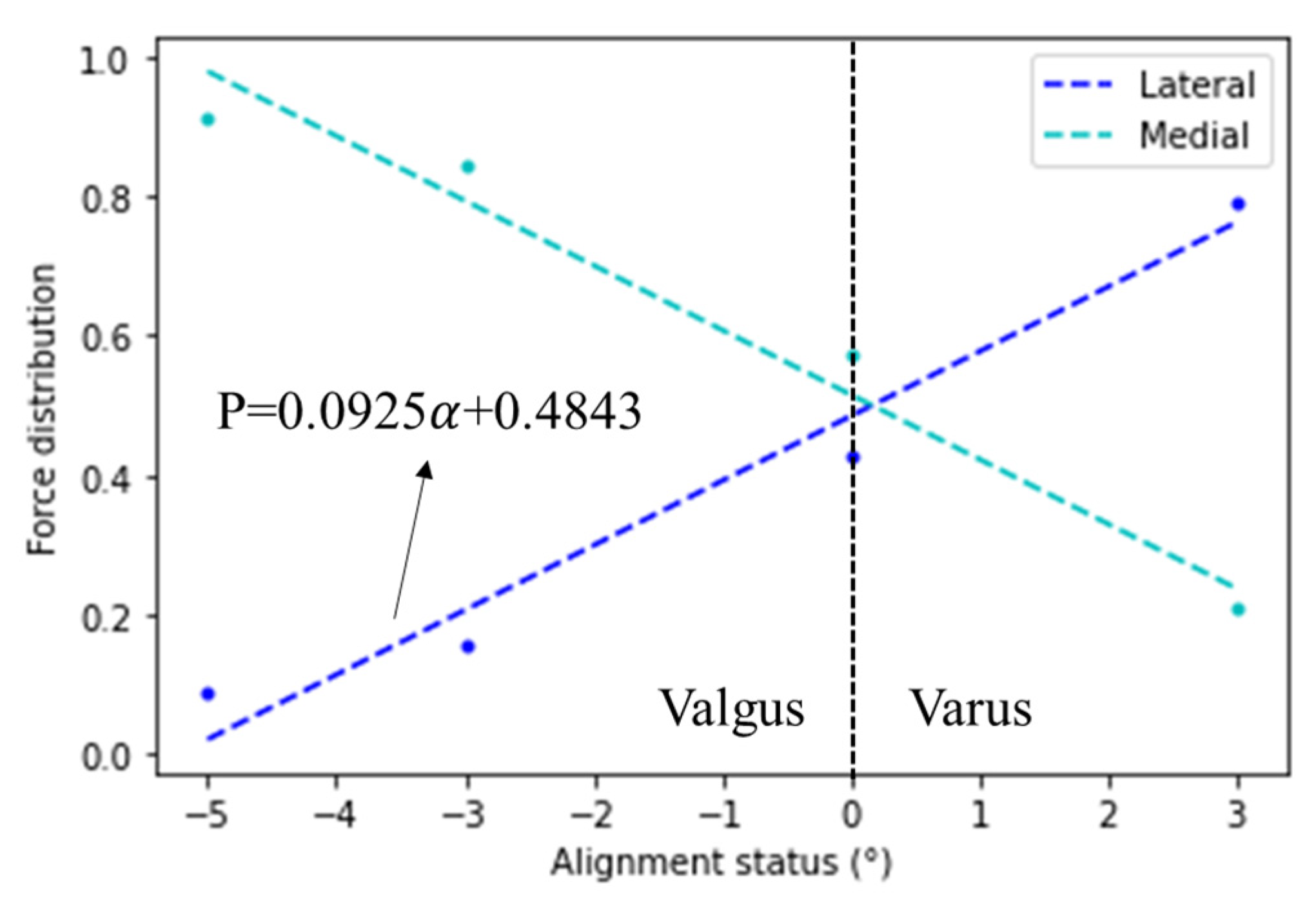
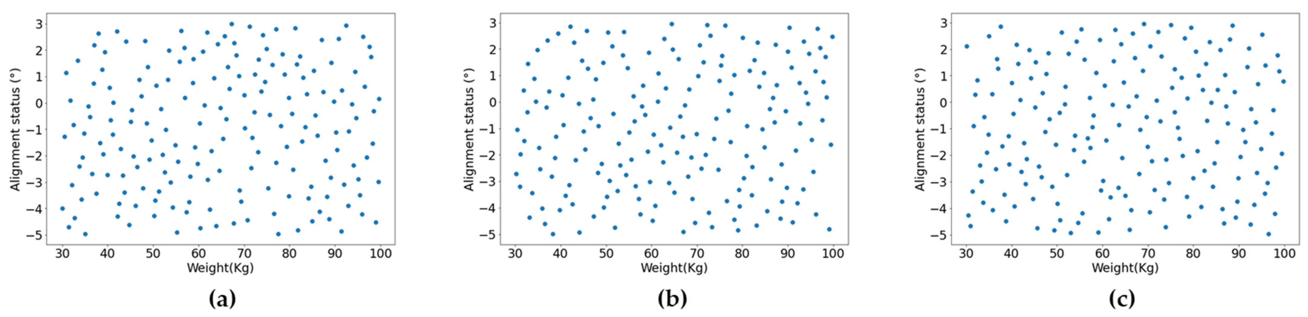
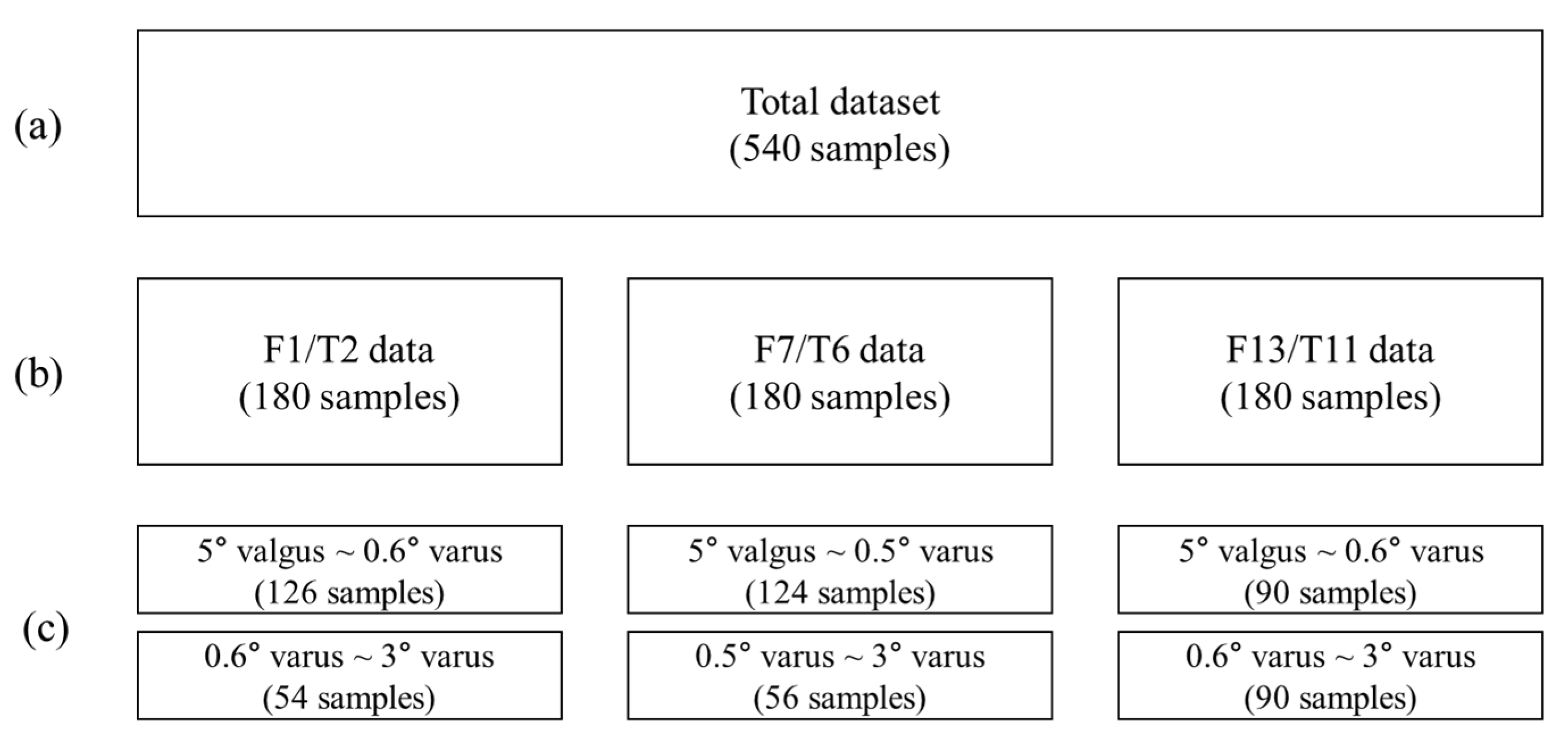
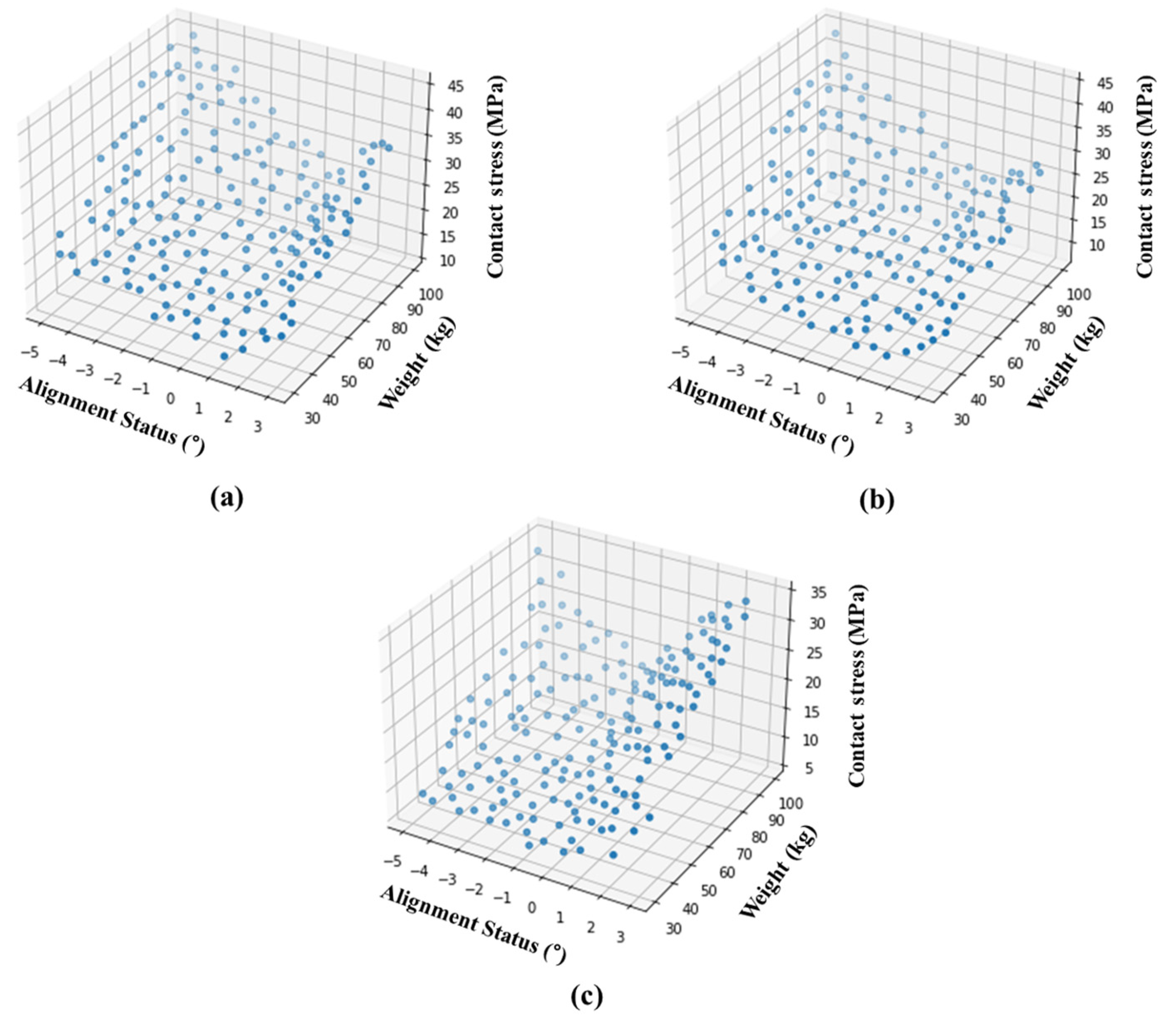
3.2. Results of Data Generation
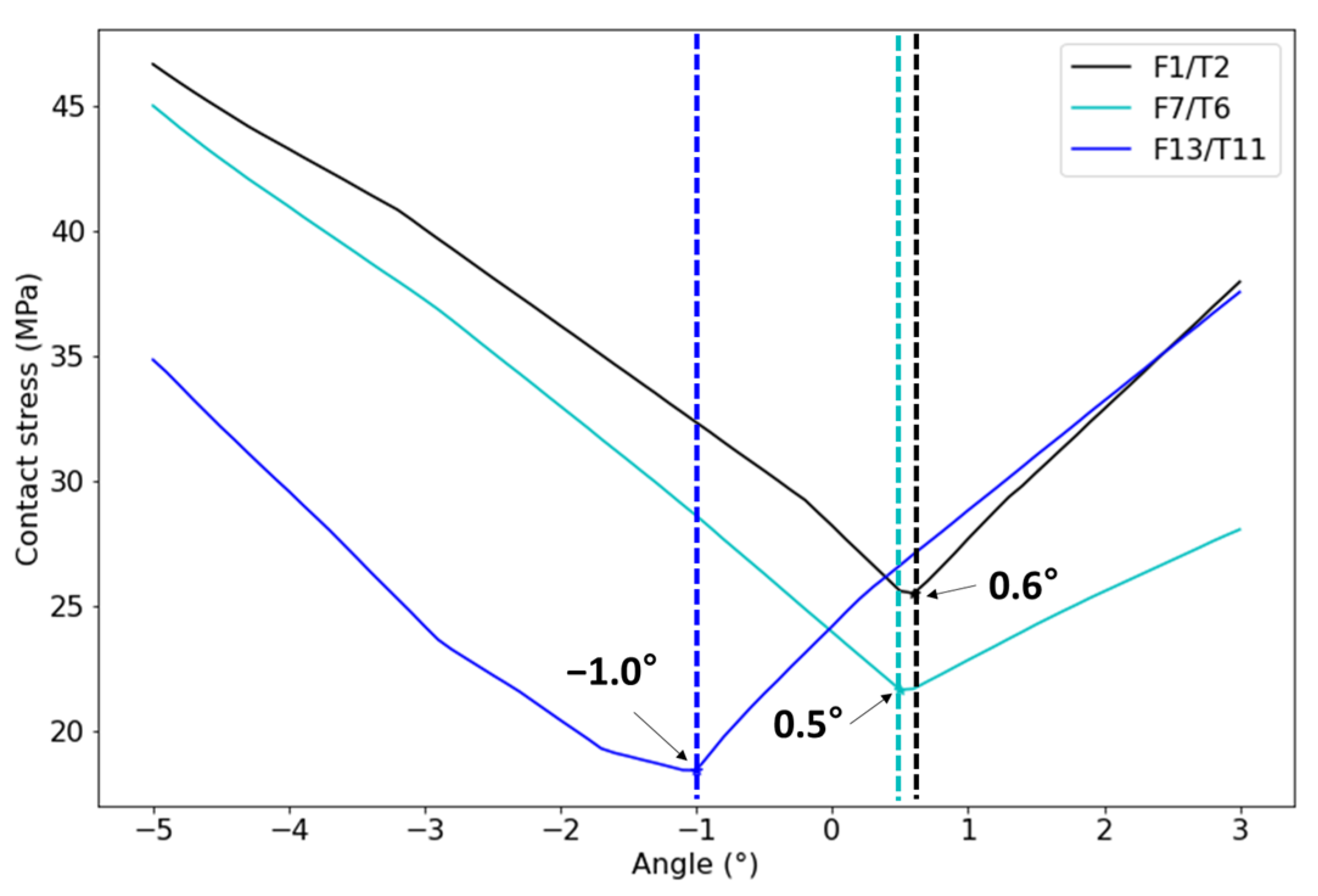
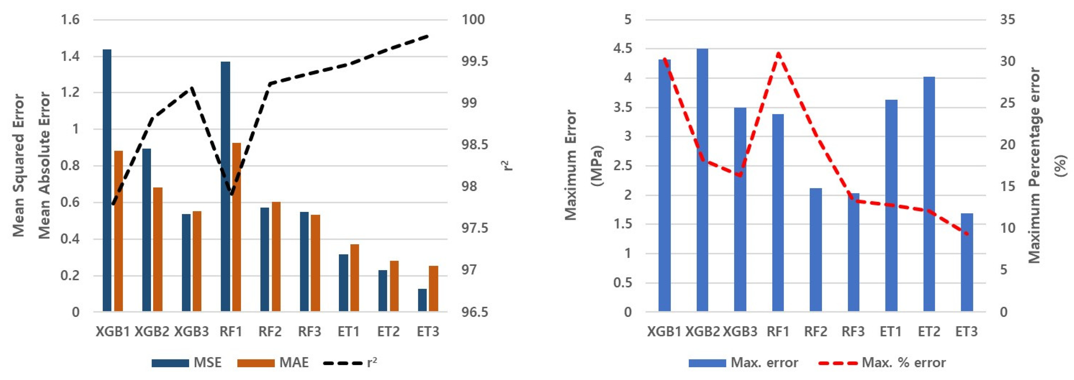
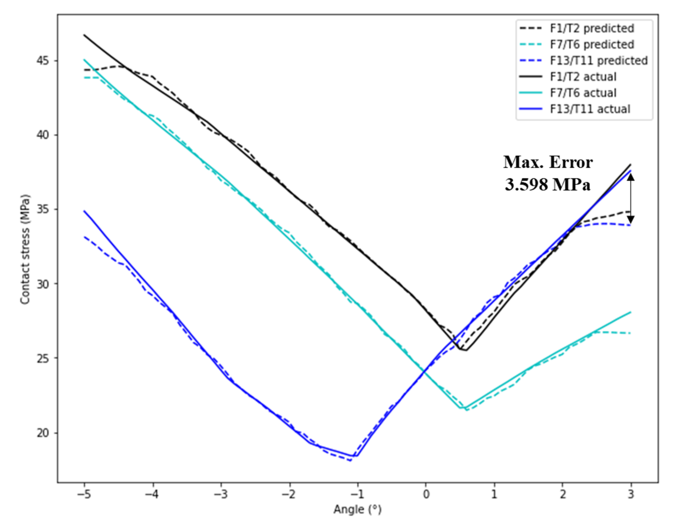
3.3. Results of Contact Stress Prediction
4. Conclusions
Author Contributions
Funding
Data Availability Statement
Conflicts of Interest
References
- Rajgopal, A.; Ahuja, N.; Dolai, B. Total Knee Arthroplasty in Stiff and Ankylosed Knees. J. Arthroplast. 2005, 20, 585–590. [Google Scholar] [CrossRef]
- Boulos, A.; Lemme, N. Total Knee Arthroplasty. In Essential Orthopedic Review; Springer: Cham, Switzerland, 2018; pp. 165–168. [Google Scholar] [CrossRef]
- Bae, D.K.; Song, S.J. Computer Assisted Navigation in Knee Arthroplasty. Clin. Orthop. Surg. 2011, 3, 259–267. [Google Scholar] [CrossRef] [PubMed]
- Stulberg, S.D.; Yaffe, M.A.; Koo, S.S. Computer-Assisted Surgery versus Manual Total Knee Arthroplasty: A Case-Controlled Study. J. Bone Jt. Surg. 2006, 88, 47–54. [Google Scholar] [CrossRef]
- Tabatabaee, R.M.; Rasouli, M.R.; Maltenfort, M.G.; Fuino, R.; Restrepo, C.; Oliashirazi, A. Computer-Assisted Total Knee Arthroplasty: Is There a Difference Between Image-Based and Imageless Techniques? J. Arthroplast. 2018, 33, 1076–1081. [Google Scholar] [CrossRef] [PubMed]
- Kurtz, S.; Ong, K.; Lau, E.; Mowat, F.; Halpern, M. Projections of Primary and Revision Hip and Knee Arthroplasty in the United States from 2005 to 2030. J. Bone Jt. Surg. 2007, 89, 780–785. [Google Scholar] [CrossRef]
- Schroer, W.C.; Berend, K.R.; Lombardi, A.V.; Barnes, C.L.; Bolognesi, M.P.; Berend, M.E.; Ritter, M.A.; Nunley, R.M. Why Are Total Knees Failing Today? Etiology of Total Knee Revision in 2010 and 2011. J. Arthroplast. 2013, 28, 116–119. [Google Scholar] [CrossRef]
- Sadoghi, P.; Liebensteiner, M.; Agreiter, M.; Leithner, A.; Böhler, N.; Labek, G. Revision Surgery after Total Joint Arthroplasty: A Complication-Based Analysis Using Worldwide Arthroplasty Registers. J. Arthroplast. 2013, 28, 1329–1332. [Google Scholar] [CrossRef]
- Mullaji, A.; Kanna, R.; Marawar, S.; Kohli, A.; Sharma, A. Comparison of Limb and Component Alignment Using Computer-Assisted Navigation Versus Image Intensifier-Guided Conventional Total Knee Arthroplasty.A Prospective, Randomized, Single-Surgeon Study of 467 Knees. J. Arthroplast. 2007, 22, 953–959. [Google Scholar] [CrossRef]
- Schmitt, J.; Hauk, C.; Kienapfel, H.; Pfeiffer, M.; Efe, T.; Fuchs-Winkelmann, S.; Heyse, T.J. Navigation of Total Knee Arthroplasty: Rotation of Components and Clinical Results in a Prospectively Randomized Study. BMC Musculoskelet. Disord. 2011, 12, 16. [Google Scholar] [CrossRef] [Green Version]
- Davis, E.T.; Pagkalos, J.; Gallie, P.A.M.; Macgroarty, K.; Waddell, J.P.; Schemitsch, E.H. Defining the Errors in the Registration Process During Imageless Computer Navigation in Total Knee Arthroplasty: A Cadaveric Study. J. Arthroplast. 2014, 29, 698–701. [Google Scholar] [CrossRef]
- D’Lima, D.D.; Patil, S.; Steklov, N.; Slamin, J.E.; Colwell, C.W. Tibial Forces Measured In Vivo after Total Knee Arthroplasty. J. Arthroplast. 2006, 21, 255–262. [Google Scholar] [CrossRef] [PubMed]
- Srivastava, A.; Lee, G.Y.; Steklov, N.; Colwell, C.W.; Ezzet, K.A.; D’Lima, D.D. Effect of Tibial Component Varus on Wear in Total Knee Arthroplasty. Knee 2012, 19, 560–563. [Google Scholar] [CrossRef] [PubMed]
- Catani, F.; Innocenti, B.; Belvedere, C.; Labey, L.; Ensini, A.; Leardini, A. The Mark Coventry Award Articular: Contact Estimation in TKA Using in Vivo Kinematics and Finite Element Analysis. Clin. Orthop. Relat. Res. 2010, 468, 19–28. [Google Scholar] [CrossRef] [Green Version]
- Innocenti, B.; Labey, L.; Kamali, A.; Pascale, W.; Pianigiani, S. Development and Validation of a Wear Model to Predict Polyethylene Wear in a Total Knee Arthroplasty: A Finite Element Analysis. Lubricants 2014, 2, 193–205. [Google Scholar] [CrossRef] [Green Version]
- Arab, A.Z.E.A.; Merdji, A.; Benaissa, A.; Roy, S.; Bachir Bouiadjra, B.A.; Layadi, K.; Ouddane, A.; Mukdadi, O.M. Finite-Element Analysis of a Lateral Femoro-Tibial Impact on the Total Knee Arthroplasty. Comput. Methods Programs Biomed. 2020, 192, 105446. [Google Scholar] [CrossRef]
- Suh, D.S.; Kang, K.T.; Son, J.; Kwon, O.R.; Baek, C.; Koh, Y.G. Computational Study on the Effect of Malalignment of the Tibial Component on the Biomechanics of Total Knee Arthroplasty: A Finite Element Analysis. Bone Jt. Res. 2017, 6, 623–630. [Google Scholar] [CrossRef] [PubMed]
- Kang, K.T.; Son, J.; Kwon, S.K.; Kwon, O.R.; Park, J.H.; Koh, Y.G. Finite Element Analysis for the Biomechanical Effect of Tibial Insert Materials in Total Knee Arthroplasty. Compos. Struct. 2018, 201, 141–150. [Google Scholar] [CrossRef]
- Gheorghiu, N.; Socea, B.; Dimitriu, M.; Bacalbasa, N.; Stan, G.; Orban, H. A Finite Element Analysis for Predicting Outcomes of Cemented Total Knee Arthroplasty. Exp. Ther. Med. 2021, 21, 267. [Google Scholar] [CrossRef] [PubMed]
- Woiczinski, M.; Steinbrück, A.; Weber, P.; Müller, P.E.; Jansson, V.; Schröder, C. Development and Validation of a Weight-Bearing Finite Element Model for Total Knee Replacement. Comput. Methods Biomech. Biomed. Engin. 2016, 19, 1033–1045. [Google Scholar] [CrossRef] [PubMed]
- Lee, Y.S.; Lee, T.Q.; Keyak, J.H. Effect of an UHMWPE Patellar Component on Stress Fields in the Patella: A Finite Element Analysis. Knee Surg. Sport. Traumatol. Arthrosc. 2009, 17, 71–82. [Google Scholar] [CrossRef]
- Miller, M.D.; Thompson, S.R.; Hart, J. Review of Orthopaedics E-Book; Elsevier Health Sciences: Amsterdam, The Netherlands, 2012. [Google Scholar]
- Díaz-Alcaide, S.; Martínez-Santos, P. Mapping Fecal Pollution in Rural Groundwater Supplies by Means of Artificial Intelligence Classifiers. J. Hydrol. 2019, 577, 124006. [Google Scholar] [CrossRef]
- Merali, Z.G.; Witiw, C.D.; Badhiwala, J.H.; Wilson, J.R.; Fehlings, M.G. Using a Machine Learning Approach to Predict Outcome after Surgery for Degenerative Cervical Myelopathy. PLoS ONE 2019, 14, e0215133. [Google Scholar] [CrossRef] [PubMed]
- Hayward, J.; Alvarez, S.A.; Ruiz, C.; Sullivan, M.; Tseng, J.; Whalen, G. Machine Learning of Clinical Performance in a Pancreatic Cancer Database. Artif. Intell. Med. 2010, 49, 187–195. [Google Scholar] [CrossRef] [PubMed]
- Allyn, J.; Allou, N.; Augustin, P.; Philip, I.; Martinet, O.; Belghiti, M.; Provenchere, S.; Montravers, P.; Ferdynus, C. A Comparison of a Machine Learning Model with EuroSCORE II in Predicting Mortality after Elective Cardiac Surgery: A Decision Curve Analysis. PLoS ONE 2017, 12, e0169772. [Google Scholar] [CrossRef] [PubMed] [Green Version]
- Arvind, V.; Kim, J.S.; Oermann, E.K.; Kaji, D.; Cho, S.K. Predicting Surgical Complications in Adult Patients Undergoing Anterior Cervical Discectomy and Fusion Using Machine Learning. Neurospine 2018, 15, 329–337. [Google Scholar] [CrossRef]
- Qin, J.; Chen, L.; Liu, Y.; Liu, C.; Feng, C.; Chen, B. A Machine Learning Methodology for Diagnosing Chronic Kidney Disease. IEEE Access 2020, 8, 20991–21002. [Google Scholar] [CrossRef]
- Geurts, P.; Ernst, D.; Wehenkel, L. Extremely Randomized Trees. Mach. Learn. 2006, 63, 3–42. [Google Scholar] [CrossRef] [Green Version]
- Gotz, M.; Weber, C.; Blocher, J.; Stieltjes, B.; Meinzer, H.; Maier-Hein, K. Extremely Randomized Trees Based Brain Tumor Segmentation. Proceeding BRATS Chall.-MICCAI 2014, 14, 6–11. [Google Scholar]
- Alawadi, S.; Mera, D.; Fernández-Delgado, M.; Alkhabbas, F.; Olsson, C.M.; Davidsson, P. A Comparison of Machine Learning Algorithms for Forecasting Indoor Temperature in Smart Buildings. Energy Syst. 2022, 13, 689–705. [Google Scholar] [CrossRef] [Green Version]
- Damaševičius, R.; Venčkauskas, A.; Toldinas, J.; Grigaliūnas, Š. Ensemble-based Classification Using Neural Networks and Machine Learning Models for Windows Pe Malware Detection. Electronics 2021, 10, 485. [Google Scholar] [CrossRef]
- Jun, Z.; Youqiang, Z.; Wei, C.; Fu, C. Research on Prediction of Contact Stress of Acetabular Lining Based on Principal Component Analysis and Support Vector Regression. Biotechnol. Biotechnol. Equip. 2021, 35, 462–468. [Google Scholar] [CrossRef]
- Kruse, C.; Eiken, P.; Vestergaard, P. Machine Learning Principles Can Improve Hip Fracture Prediction. Calcif. Tissue Int. 2017, 100, 348–360. [Google Scholar] [CrossRef] [PubMed]
- Chen, T.; Guestrin, C. XGBoost: A Scalable Tree Boosting System. In Proceedings of the the 22nd ACM SIGKDD International Conference on Knowledge Discovery and Data Mining, San Francisco, CA, USA, 13–17 August 2016; pp. 785–794. [Google Scholar] [CrossRef] [Green Version]
- Breiman, L. Random Forests. Mach. Learn. 2001, 45, 5–32. [Google Scholar] [CrossRef] [Green Version]
- Noble, W.S. What Is a Support Vector Machine? Nat. Biotechnol. 2006, 24, 1565–1567. [Google Scholar] [CrossRef] [PubMed]
- Gao, S.; Li, H. Breast Cancer Diagnosis Based on Support Vector Machine. In Proceedings of the 2012 2nd International Conference on Uncertainty Reasoning and Knowledge Engineering, Jalarta, Indonesia, 14–15 August 2012; pp. 240–243. [Google Scholar] [CrossRef]
- Lin, W.; Tian, X.; Lu, X.; Ma, D.; Wu, Y.; Hong, J.; Yan, R.; Feng, G.; Cheng, Z. Prediction of Bedridden Duration of Hospitalized Patients by Machine Learning Based on EMRS at Admission. CIN Comput. Inform. Nurs. 2022, 40, 251–257. [Google Scholar] [CrossRef] [PubMed]
- Jin, R.; Chen, W.; Sudjianto, A. An Efficient Algorithm for Constructing Optimal Designs of Computer Experiments. Int. Des. Eng. Tech. Conf. Comput. Inf. Eng. Conf. 2003, 37009, 545–554. [Google Scholar]
- Schwarzkopf, R.; Meftah, M.; Marwin, S.E.; Zabat, M.A.; Muir, J.M.; Lamb, I.R. The Use of Imageless Navigation to Quantify Cutting Error in Total Knee Arthroplasty. Knee Surg. Relat. Res. 2021, 33, 43. [Google Scholar] [CrossRef]
- Sohail, M.; Park, J.; Kim, J.Y.; Kim, H.S.; Lee, J. Modified Whiteside’s Line-Based Transepicondylar Axis for Imageless Total Knee Arthroplasty. Mathematics 2022, 10, 3670. [Google Scholar] [CrossRef]
- Sershon, R.A.; Courtney, P.M.; Rosenthal, B.D.; Sporer, S.M.; Levine, B.R. Can Demographic Variables Accurately Predict Component Sizing in Primary Total Knee Arthroplasty? J. Arthroplast. 2017, 32, 3004–3008. [Google Scholar] [CrossRef]
- Kang, K.T.; Koh, Y.G.; Son, J.; Kwon, O.R.; Lee, J.S.; Kwon, S.K. Influence of Increased Posterior Tibial Slope in Total Knee Arthroplasty on Knee Joint Biomechanics: A Computational Simulation Study. J. Arthroplast. 2018, 33, 572–579. [Google Scholar] [CrossRef]
- Estupinan, J.A.; Bartel, D.L.; Wright, T.M. Residual Stresses in Ultra-High Molecular Weight Polyethylene Loaded Cyclically by a Rigid Moving Indenter in Nonconforming Geometries. J. Orthop. Res. 1998, 16, 80–88. [Google Scholar] [CrossRef] [PubMed]
- Sathasivam, S.; Walker, P.S. A Computer Model with Surface Friction for the Prediction of Total Knee Kinematics. J. Biomech. 1997, 30, 177–184. [Google Scholar] [CrossRef] [PubMed]
- Patil, N.A.; Njuguna, J.; Kandasubramanian, B. UHMWPE for Biomedical Applications: Performance and Functionalization. Eur. Polym. J. 2020, 125, 109529. [Google Scholar] [CrossRef]
- Godest, A.C.; Beaugonin, M.; Haug, E.; Taylor, M.; Gregson, P.J. Simulation of a Knee Joint Replacement during a Gait Cycle Using Explicit Finite Element Analysis. J. Biomech. 2002, 35, 267–275. [Google Scholar] [CrossRef]
- Knight, L.A.; Pal, S.; Coleman, J.C.; Bronson, F.; Haider, H.; Levine, D.L.; Taylor, M.; Rullkoetter, P.J. Comparison of Long-Term Numerical and Experimental Total Knee Replacement Wear during Simulated Gait Loading. J. Biomech. 2007, 40, 1550–1558. [Google Scholar] [CrossRef]
- Innocenti, B.; Truyens, E.; Labey, L.; Wong, P.; Victor, J.; Bellemans, J. Can Medio-Lateral Baseplate Position and Load Sharing Induce Asymptomatic Local Bone Resorption of the Proximal Tibia? A Finite Element Study. J. Orthop. Surg. Res. 2009, 4, 26. [Google Scholar] [CrossRef] [Green Version]
- Werner, F.W.; Ayers, D.C.; Maletsky, L.P.; Rullkoetter, P.J. The Effect of Valgus/Varus Malalignment on Load Distribution in Total Knee Replacements. J. Biomech. 2005, 38, 349–355. [Google Scholar] [CrossRef]
- Morrison, J.B. The Mechanics of the Knee Joint in Relation to Normal Walking. J. Biomech. 1970, 3, 51–61. [Google Scholar] [CrossRef]
- Kvålseth, T.O. Cautionary Note about R2. Am. Stat. 1985, 39, 279–285. [Google Scholar] [CrossRef]
- Hodson, T.O. Root-Mean-Square Error (RMSE) or Mean Absolute Error (MAE): When to Use Them or Not. Geosci. Model Dev. 2022, 15, 5481–5487. [Google Scholar] [CrossRef]


| Algorithm | Working Principle |
|---|---|
| XGB | Ensemble of decision trees; loss function of second-order Taylor expansion [35]. |
| RF | Ensemble of decision trees; increased diversity of the trees through the bagging procedure [36]. |
| SVM | Predicts a continuous output while maximizing the margin between the classes [37]. |
| ET | Ensemble of decision trees; a more randomized sampling method compared to RF [29]. |
| Set | F1/T2 | F7/T6 | F13/T11 |
|---|---|---|---|
| AP length (mm) | 50/36 | 62/44 | 76/57 |
| ML length (mm) | 59/57 | 67/69 | 78/86 |
| Young’s Modulus (MPa) | Poisson’s Ratio | |
|---|---|---|
| Ti6Al4V alloy | 110,000 | 0.30 |
| UHMWPE | 685 | 0.47 |
| Set | F1/T2 | F7/T6 | F13/T11 |
|---|---|---|---|
| Femoral component | 15,909 | 29,866 | 34,347 |
| Plastic spacer | 9448 | 13,529 | 23,598 |
| Total | 25,357 | 43,395 | 57,945 |
| MAE | MSE | r2 (%) | Max. Error (MPa) | Max. % Error (%) |
|---|---|---|---|---|
| 0.1281 | 0.2536 | 99.80 | 1.689 | 9.398 |
Disclaimer/Publisher’s Note: The statements, opinions and data contained in all publications are solely those of the individual author(s) and contributor(s) and not of MDPI and/or the editor(s). MDPI and/or the editor(s) disclaim responsibility for any injury to people or property resulting from any ideas, methods, instructions or products referred to in the content. |
© 2023 by the authors. Licensee MDPI, Basel, Switzerland. This article is an open access article distributed under the terms and conditions of the Creative Commons Attribution (CC BY) license (https://creativecommons.org/licenses/by/4.0/).
Share and Cite
Kim, J.Y.; Sohail, M.; Kim, H.S. Rapid Estimation of Contact Stresses in Imageless Total Knee Arthroplasty. Mathematics 2023, 11, 3527. https://doi.org/10.3390/math11163527
Kim JY, Sohail M, Kim HS. Rapid Estimation of Contact Stresses in Imageless Total Knee Arthroplasty. Mathematics. 2023; 11(16):3527. https://doi.org/10.3390/math11163527
Chicago/Turabian StyleKim, Jun Young, Muhammad Sohail, and Heung Soo Kim. 2023. "Rapid Estimation of Contact Stresses in Imageless Total Knee Arthroplasty" Mathematics 11, no. 16: 3527. https://doi.org/10.3390/math11163527