
Combining the Taguchi Method and Convolutional Neural Networks for Arrhythmia Classification by Using ECG Images with Single Heartbeats

Abstract
:1. Introduction
- Combining the Taguchi method and CNNs for arrhythmia classification.
- Comparing the classification results with and without electrocardiograph denoising.
- Parameter setting using orthogonal arrays in the convolution layers and max-pooling layers of the CNN.
- Successfully classifies fifteen different types of heartbeats into five major classes.
- Using ECG images with single heartbeats without feature extraction or signal conversion.
2. Materials and Methods
2.1. Data Used
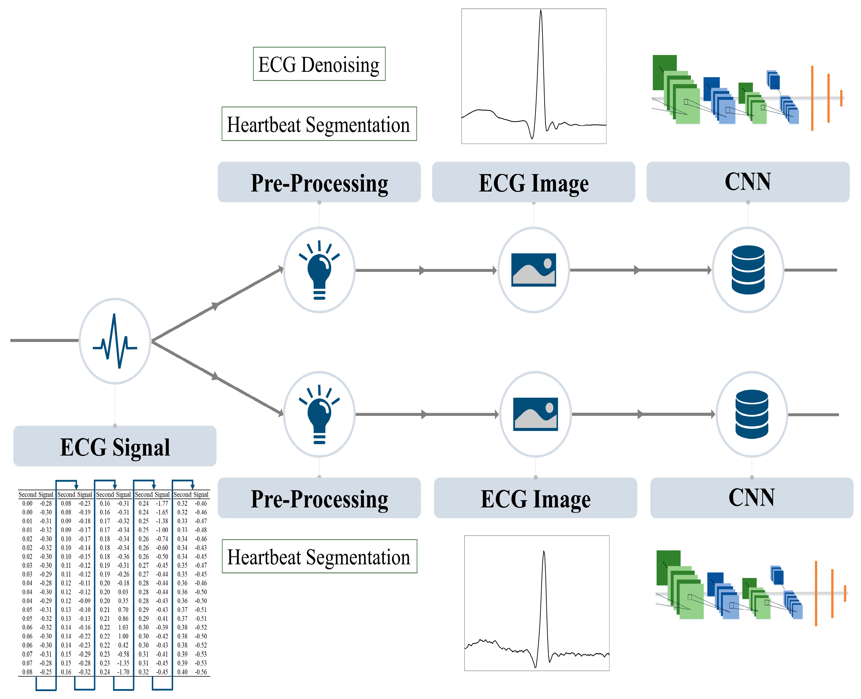
2.2. Preprocessing
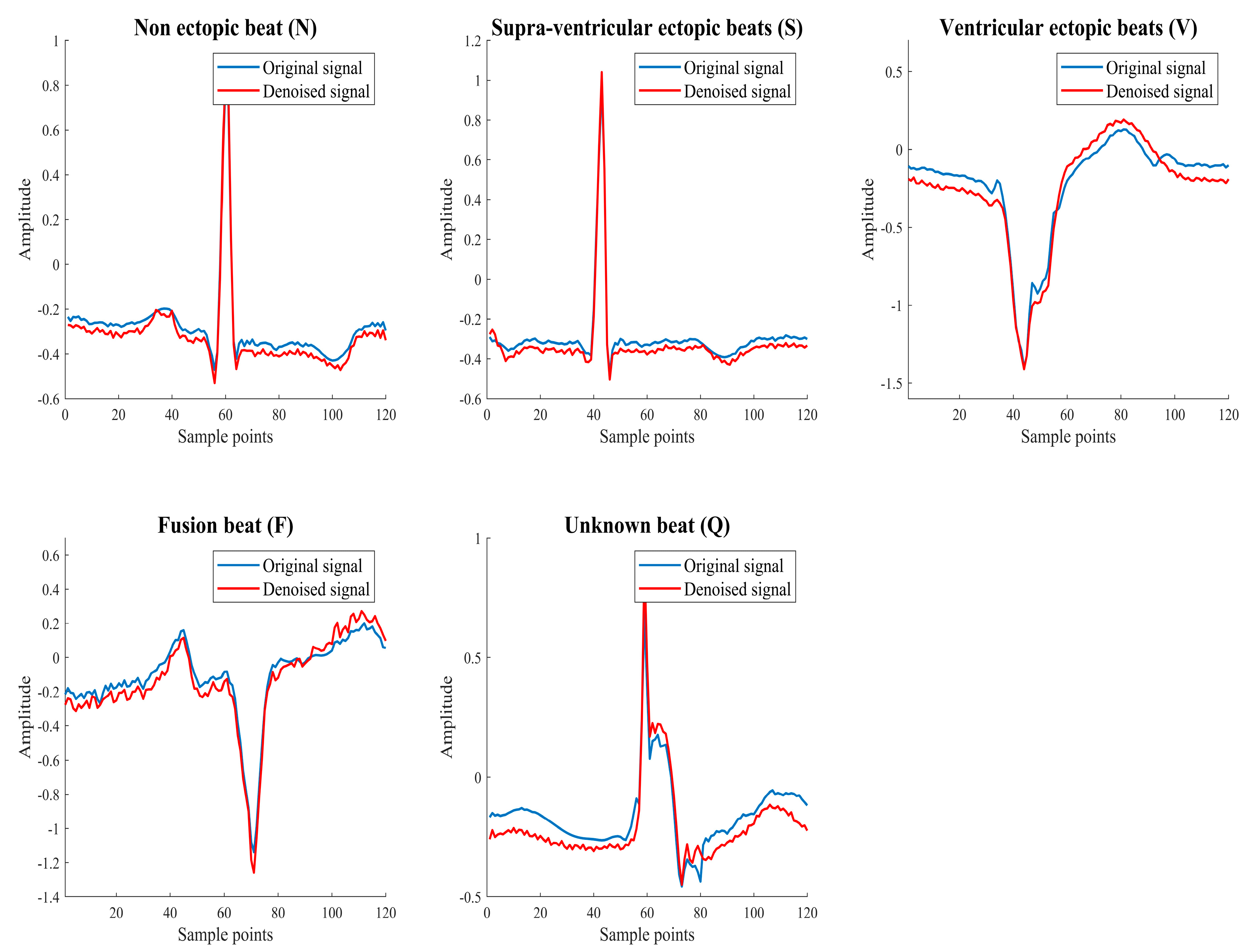
2.2.1. Electrocardiograph Denoising
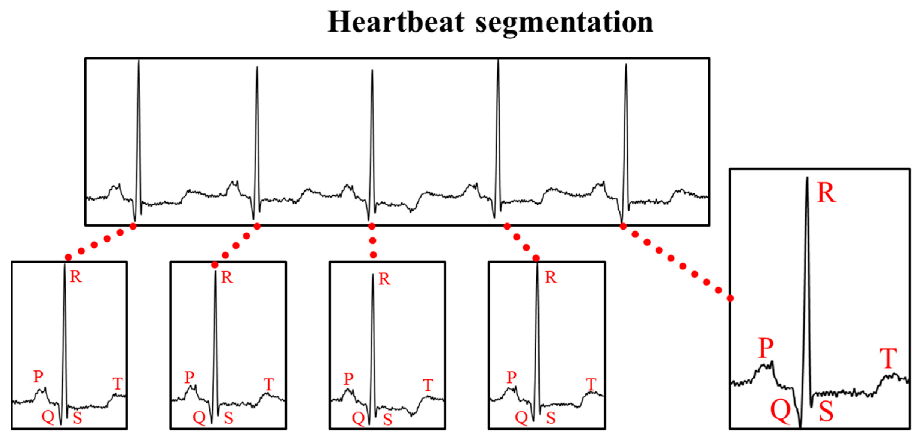
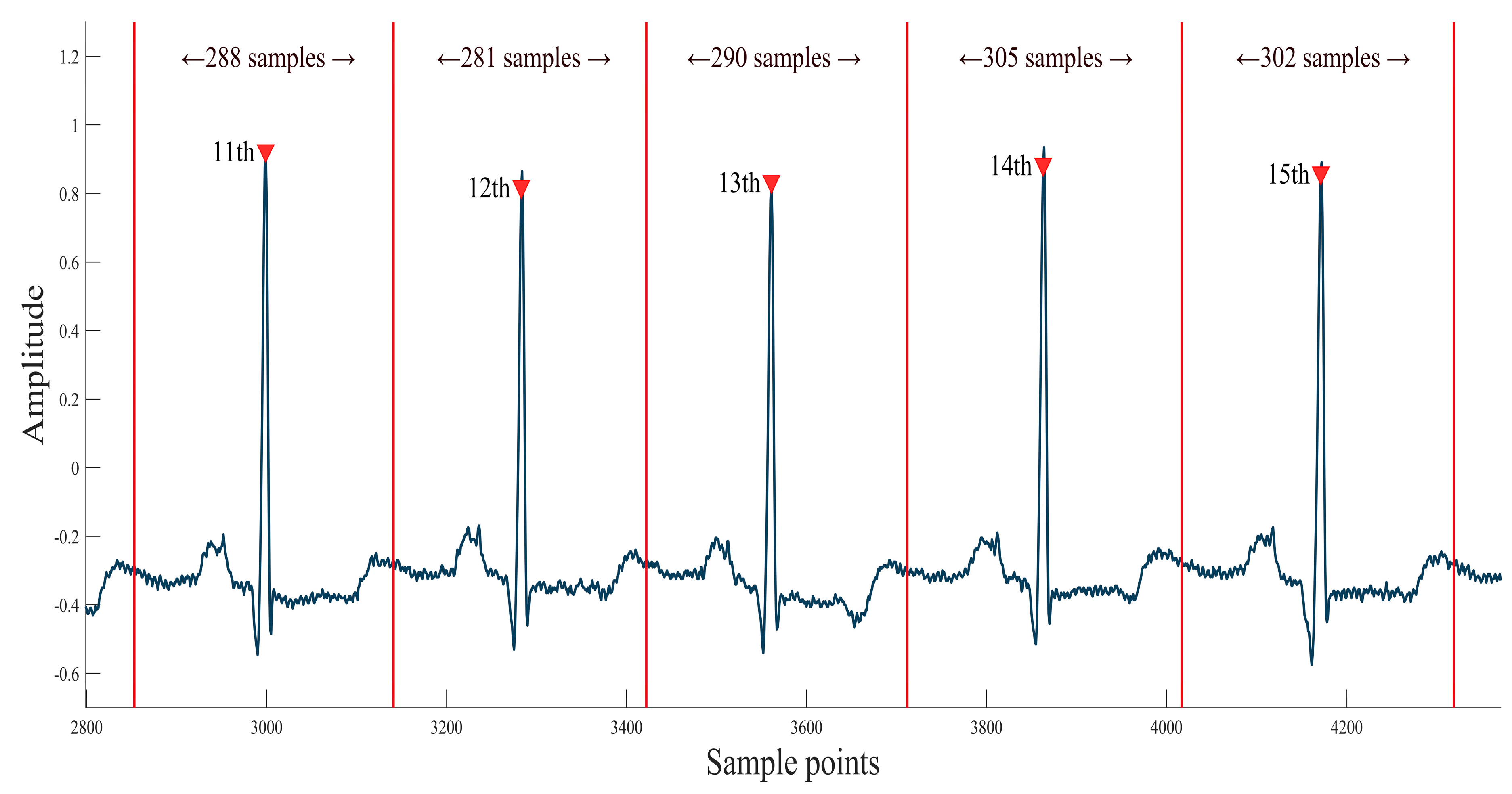
2.2.2. Heartbeat Segmentation
2.3. Creating an Image Dataset
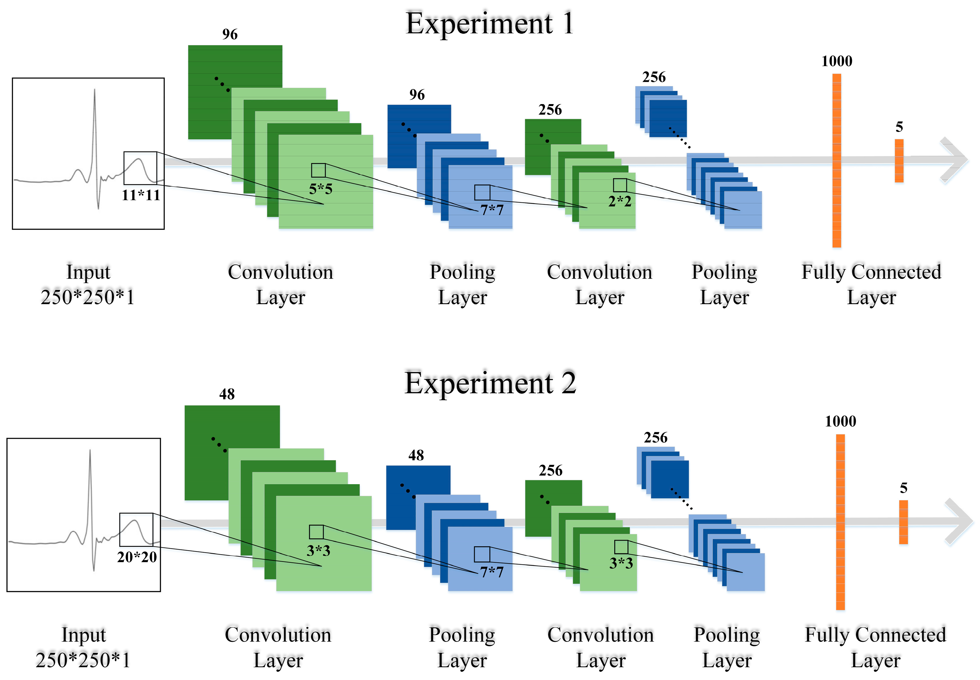
2.4. Convolutional Neural Network
2.4.1. Image Input Layer
2.4.2. Convolution Layers
2.4.3. Max-Pooling Layers
2.4.4. Fully Connected Layers
2.4.5. Softmax Layer
3. Results
3.1. Preprocessing
3.1.1. ECG Denoising
3.1.2. Heartbeat Segmentation
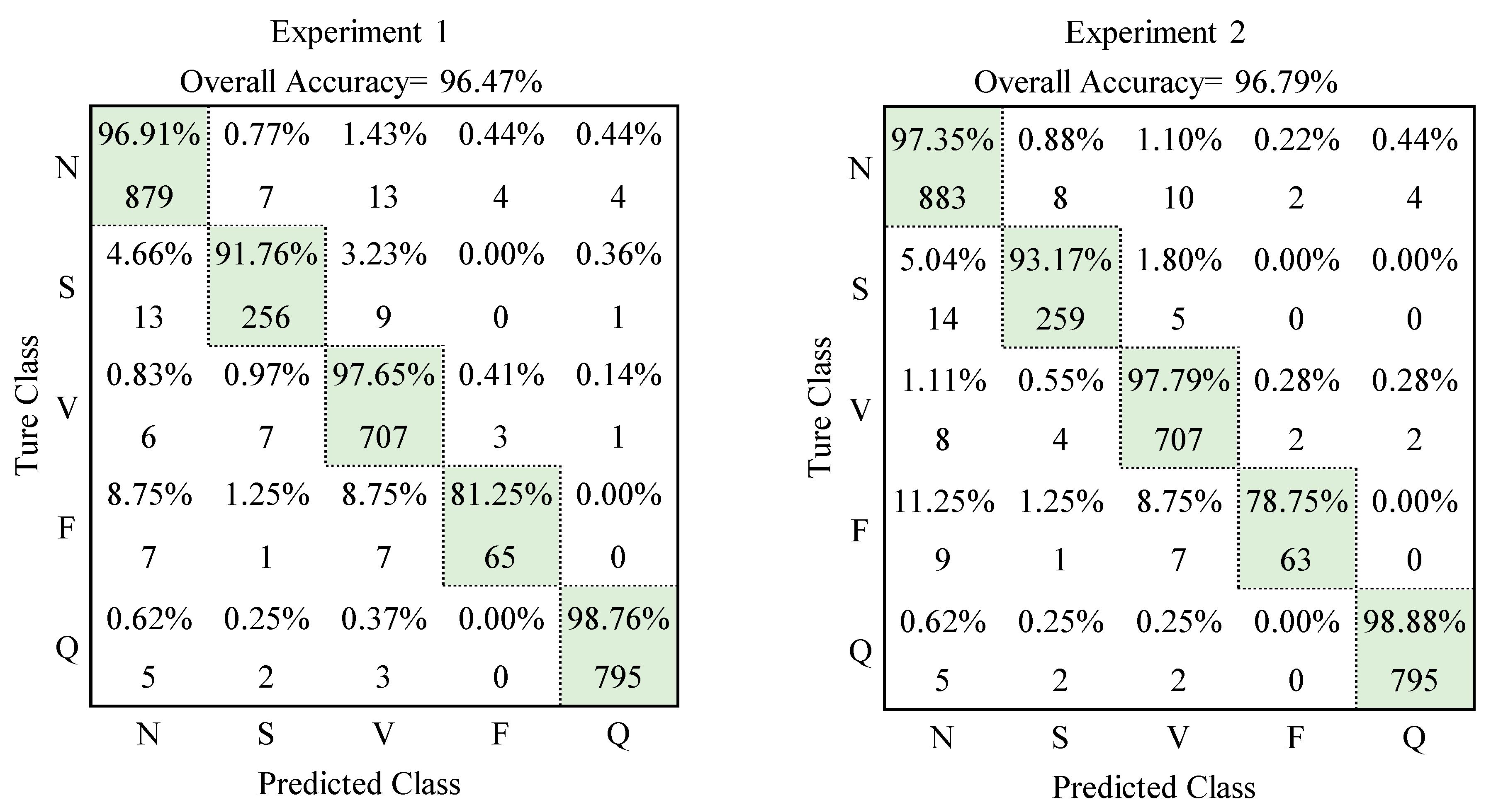
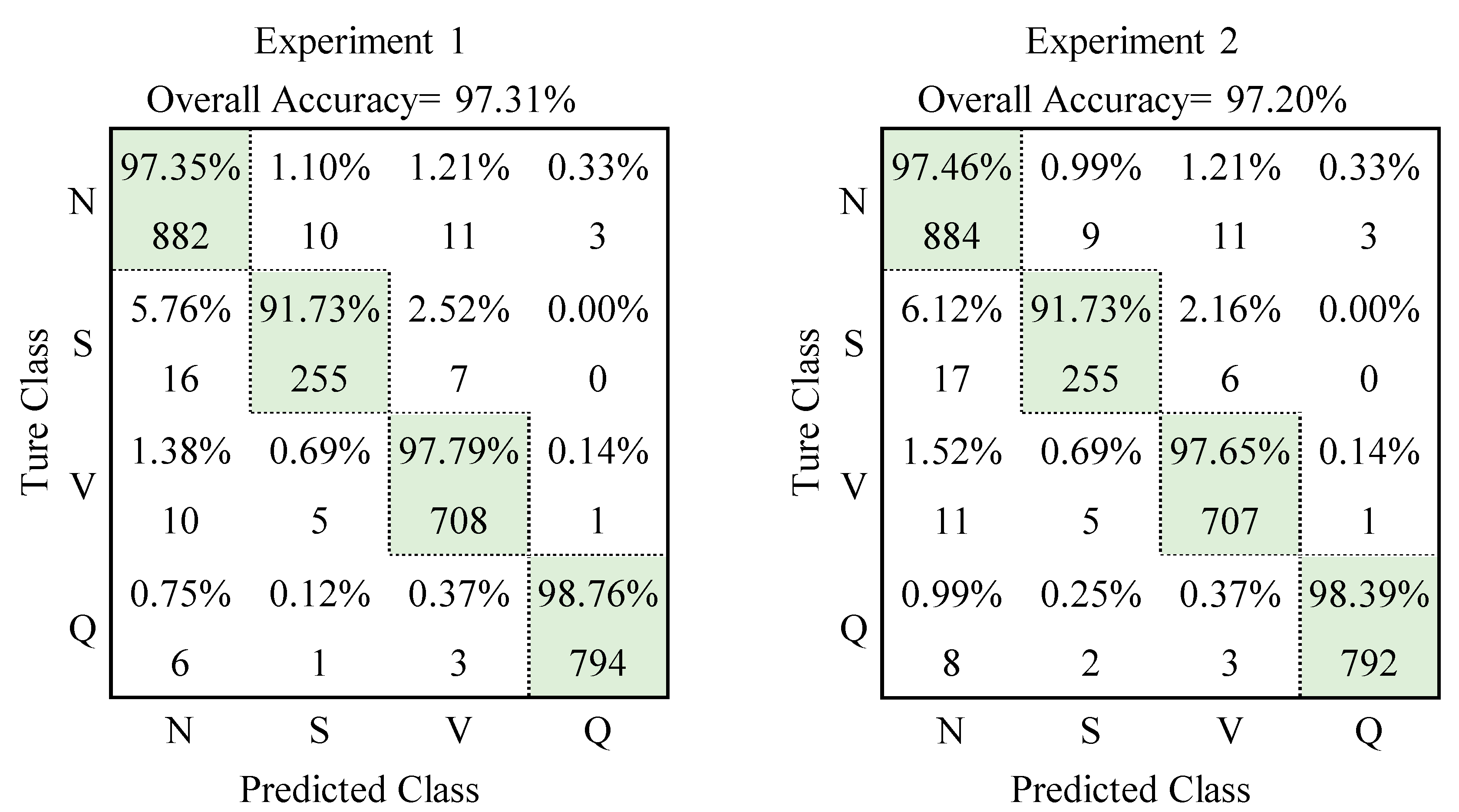
3.2. Convolutional Neural Network
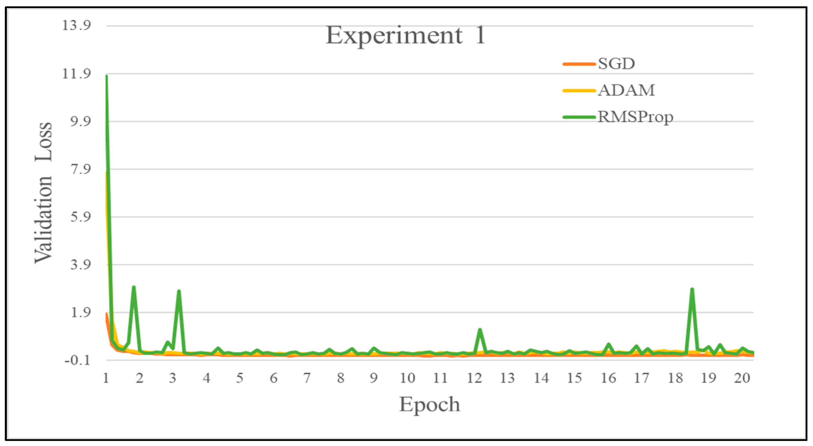
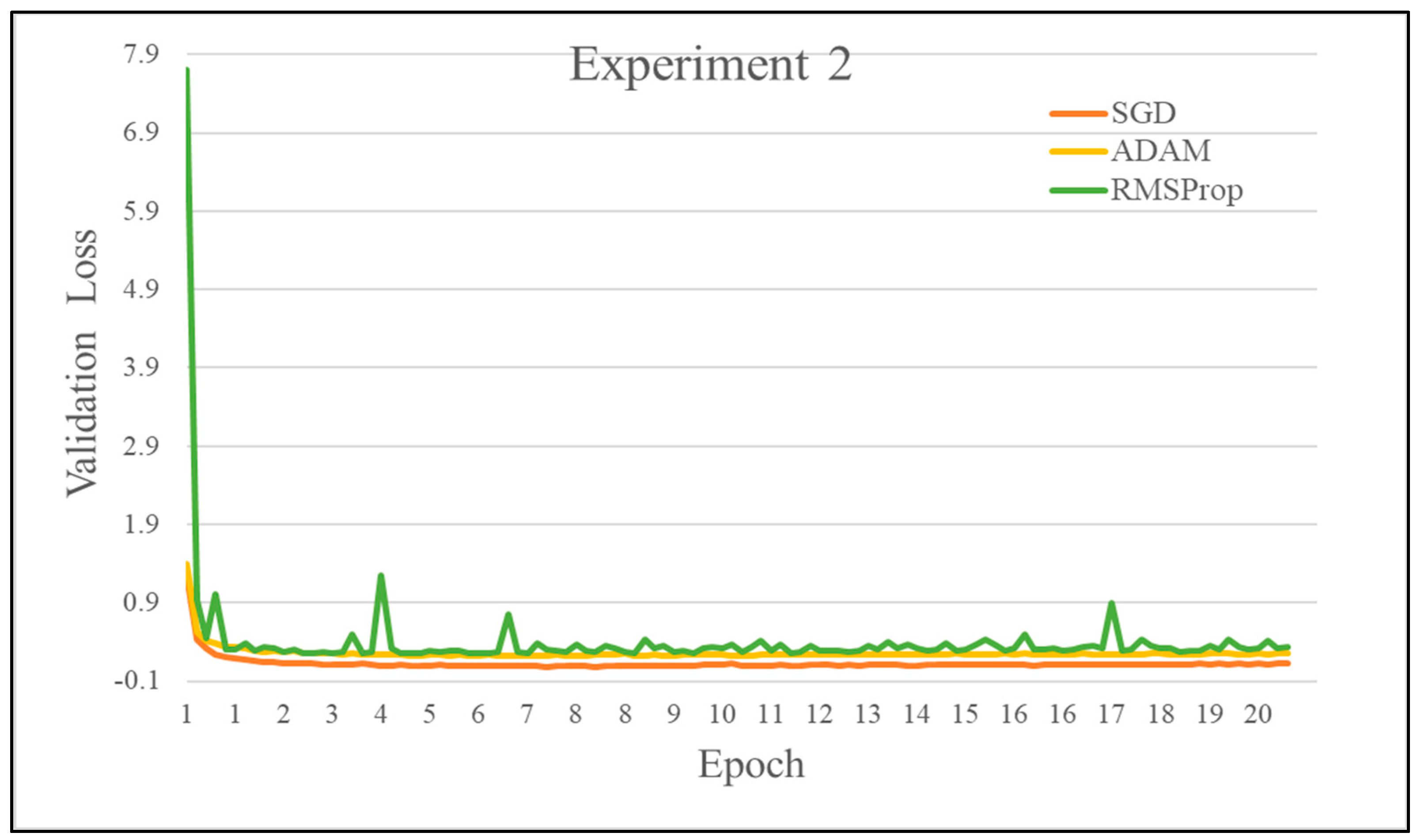
3.3. Comparison of Optimizers
4. Discussion
5. Conclusions
Author Contributions
Funding
Data Availability Statement
Acknowledgments
Conflicts of Interest
References
- Andersen, R.S.; Peimankar, A.; Puthusserypady, S. A deep learning approach for real-time detection of atrial fibrillation. Expert Syst. Appl. 2019, 115, 465–473. [Google Scholar] [CrossRef]
- Schmidhuber, J. Deep learning in neural networks: An overview. Neural Netw. 2015, 61, 85–117. [Google Scholar] [CrossRef] [Green Version]
- Hinton, G.E.; Osindero, S.; Teh, Y.-W. A Fast Learning Algorithm for Deep Belief Nets. Neural Comput. 2006, 18, 1527–1554. [Google Scholar] [CrossRef]
- Krizhevsky, A.; Sutskever, I.; Hinton, G.E. ImageNet classification with deep convolutional neural networks. Commun. ACM 2017, 60, 84–90. [Google Scholar] [CrossRef] [Green Version]
- Zeiler, M.D.; Fergus, R. Visualizing and Understanding Convolutional Networks. arXiv 2013, arXiv:1311.2901. [Google Scholar]
- Hou, J.; Wang, S.; Lai, Y.; Tsao, Y.; Chang, H.; Wang, H. Audio-Visual Speech Enhancement Using Multimodal Deep Convolutional Neural Networks. IEEE Trans. Emerg. Top. Comput. Intell. 2018, 2, 117–128. [Google Scholar] [CrossRef] [Green Version]
- Al-Antari, M.A.; Al-Masni, M.A.; Choi, M.T.; Han, S.M.; Kim, T.S. A fully integrated computer-aided diagnosis system for digital X-ray mammograms via deep learning detection, segmentation, and classification. Int. J. Med. Inform. 2018, 117, 44–54. [Google Scholar] [CrossRef]
- Xia, Y.; Wulan, N.; Wang, K.; Zhang, H. Detecting atrial fibrillation by deep convolutional neural networks. Comput. Biol. Med. 2018, 93, 84–92. [Google Scholar] [CrossRef]
- Al Rahhal, M.M.; Bazi, Y.; Al Zuair, M.; Othman, E.; BenJdira, B. Convolutional Neural Networks for Electrocardiogram Classification. J. Med. Biol. Eng. 2018, 38, 1014–1025. [Google Scholar] [CrossRef]
- Xu, X.; Wei, S.; Ma, C.; Luo, K.; Zhang, L.; Liu, C. Atrial Fibrillation Beat Identification Using the Combination of Modified Frequency Slice Wavelet Transform and Convolutional Neural Networks. J. Healthc. Eng. 2018, 2018, 2102918. [Google Scholar] [CrossRef] [Green Version]
- Wang, K.; Kumar, A. Cross-spectral iris recognition using CNN and supervised discrete hashing. Pattern Recognit. 2019, 86, 85–98. [Google Scholar] [CrossRef]
- Cao, Q.; Lin, L.; Shi, Y.; Liang, X.; Li, G. Attention-Aware Face Hallucination via Deep Reinforcement Learning. arXiv 2017, arXiv:1708.03132. [Google Scholar]
- Anthimopoulos, M.; Christodoulidis, S.; Ebner, L.; Christe, A.; Mougiakakou, S. Lung Pattern Classification for Interstitial Lung Diseases Using a Deep Convolutional Neural Network. IEEE Trans. Med. Imaging 2016, 35, 1207–1216. [Google Scholar] [CrossRef]
- Gao, F.; Wu, T.; Li, J.; Zheng, B.; Ruan, L.; Shang, D.; Patel, B. SD-CNN: A shallow-deep CNN for improved breast cancer diagnosis. Comput. Med. Imaging Graph. 2018, 70, 53–62. [Google Scholar] [CrossRef] [Green Version]
- Ragab, D.A.; Sharkas, M.; Marshall, S.; Ren, J. Breast cancer detection using deep convolutional neural networks and support vector machines. PeerJ 2019, 7, e6201. [Google Scholar] [CrossRef]
- Sudharshan, P.J.; Petitjean, C.; Spanhol, F.; Oliveira, L.E.; Heutte, L.; Honeine, P. Multiple instance learning for histopathological breast cancer image classification. Expert Syst. Appl. 2019, 117, 103–111. [Google Scholar] [CrossRef]
- Helwan, A.; El-Fakhri, G.; Sasani, H.; Uzun Ozsahin, D. Deep networks in identifying CT brain hemorrhage. J. Intell. Fuzzy Syst. 2018, 35, 2215–2228. [Google Scholar] [CrossRef]
- Acharya, U.R.; Fujita, H.; Lih, O.S.; Hagiwara, Y.; Tan, J.H.; Adam, M. Automated detection of arrhythmias using different intervals of tachycardia ECG segments with convolutional neural network. Inf. Sci. 2017, 405, 81–90. [Google Scholar] [CrossRef]
- Yildirim, O.; Plawiak, P.; Tan, R.S.; Acharya, U.R. Arrhythmia detection using deep convolutional neural network with long duration ECG signals. Comput. Biol. Med. 2018, 102, 411–420. [Google Scholar] [CrossRef]
- Faust, O.; Shenfield, A.; Kareem, M.; San, T.R.; Fujita, H.; Acharya, U.R. Automated detection of atrial fibrillation using long short-term memory network with RR interval signals. Comput. Biol. Med. 2018, 102, 327–335. [Google Scholar] [CrossRef] [Green Version]
- Oh, S.L.; Ng, E.Y.K.; Tan, R.S.; Acharya, U.R. Automated diagnosis of arrhythmia using combination of CNN and LSTM techniques with variable length heart beats. Comput. Biol. Med. 2018, 102, 278–287. [Google Scholar] [CrossRef]
- Zhao, Z.; Zhang, Y.; Deng, Y.; Zhang, X. ECG authentication system design incorporating a convolutional neural network and generalized S-Transformation. Comput. Biol. Med. 2018, 102, 168–179. [Google Scholar] [CrossRef]
- Lecun, Y.; Bottou, L.; Bengio, Y.; Haffner, P. Gradient-based learning applied to document recognition. Proc. IEEE 1998, 86, 2278–2324. [Google Scholar] [CrossRef] [Green Version]
- Simonyan, K.; Zisserman, A. Very Deep Convolutional Networks for Large-Scale Image Recognition. arXiv 2014, arXiv:1409.1556. [Google Scholar]
- Szegedy, C.; Wei, L.; Yangqing, J.; Sermanet, P.; Reed, S.; Anguelov, D.; Erhan, D.; Vanhoucke, V.; Rabinovich, A. Going deeper with convolutions. arXiv 2014, arXiv:1409.4842. [Google Scholar]
- Martis, R.J.; Acharya, U.R.; Min, L.C. ECG beat classification using PCA, LDA, ICA and Discrete Wavelet Transform. Biomed. Signal Process. Control 2013, 8, 437–448. [Google Scholar] [CrossRef]
- Martis, R.J.; Acharya, U.R.; Adeli, H.; Prasad, H.; Tan, J.H.; Chua, K.C.; Too, C.L.; Yeo, S.W.J.; Tong, L. Computer aided diagnosis of atrial arrhythmia using dimensionality reduction methods on transform domain representation. Biomed. Signal Process. Control 2014, 13, 295–305. [Google Scholar] [CrossRef]
- Khalaf, A.F.; Owis, M.I.; Yassine, I.A. A novel technique for cardiac arrhythmia classification using spectral correlation and support vector machines. Expert Syst. Appl. 2015, 42, 8361–8368. [Google Scholar] [CrossRef]
- Jung, W.H.; Lee, S.G. An Arrhythmia Classification Method in Utilizing the Weighted KNN and the Fitness Rule. Innov. Res. BioMed. Eng. 2017, 38, 138–148. [Google Scholar] [CrossRef]
- Pławiak, P. Novel methodology of cardiac health recognition based on ECG signals and evolutionary-neural system. Expert Syst. Appl. 2018, 92, 334–349. [Google Scholar] [CrossRef]
- Sharma, R.R.; Kumar, A.; Pachori, R.B.; Acharya, U.R. Accurate automated detection of congestive heart failure using eigenvalue decomposition based features extracted from HRV signals. Biocybern. Biomed. Eng. 2019, 39, 312–327. [Google Scholar] [CrossRef]
- Bhagyalakshmi, V.; Pujeri, R.V.; Devanagavi, G.D. GB-SVNN: Genetic BAT assisted support vector neural network for arrhythmia classification using ECG signals. J. King Saud Univ.—Comput. Inf. Sci. 2018, 33, 54–67. [Google Scholar] [CrossRef]
- Khazaei, M.; Raeisi, K.; Goshvarpour, A.; Ahmadzadeh, M. Early detection of sudden cardiac death using nonlinear analysis of heart rate variability. Biocybern. Biomed. Eng. 2018, 38, 931–940. [Google Scholar] [CrossRef]
- Gutiérrez-Gnecchi, J.A.; Morfin-Magaña, R.; Lorias-Espinoza, D.; Tellez-Anguiano, A.d.C.; Reyes-Archundia, E.; Méndez-Patiño, A.; Castañeda-Miranda, R. DSP-based arrhythmia classification using wavelet transform and probabilistic neural network. Biomed. Signal Process. Control 2017, 32, 44–56. [Google Scholar] [CrossRef] [Green Version]
- Lee, H.; Shin, S.-Y.; Seo, M.; Nam, G.-B.; Joo, S. Prediction of Ventricular Tachycardia One Hour before Occurrence Using Artificial Neural Networks. Sci. Rep. 2016, 6, 32390. [Google Scholar] [CrossRef]
- Pławiak, P.; Abdar, M.; Pławiak, J.; Makarenkov, V.; Acharya, U.R. DGHNL: A new deep genetic hierarchical network of learners for prediction of credit scoring. Inf. Sci. 2020, 516, 401–418. [Google Scholar] [CrossRef]
- Tuncer, T.; Dogan, S.; Pławiak, P.; Rajendra Acharya, U. Automated arrhythmia detection using novel hexadecimal local pattern and multilevel wavelet transform with ECG signals. Knowl.-Based Syst. 2019, 186, 104923. [Google Scholar] [CrossRef]
- Kandala, R.; Dhuli, R.; Pławiak, P.; Naik, G.; Moeinzadeh, H.; Gargiulo, G.; Suryanarayana, G. Towards Real-Time Heartbeat Classification: Evaluation of Nonlinear Morphological Features and Voting Method. Sensors 2019, 19, 5079. [Google Scholar] [CrossRef] [Green Version]
- Pławiak, P.; Abdar, M. Novel Methodology for Cardiac Arrhythmias Classification Based on Long-Duration ECG Signal Fragments Analysis. In Biomedical Signal Processing—Advances in Theory, Algorithms, and Applications; Springer: Singapore, 2020; pp. 225–272. [Google Scholar]
- Pławiak, P.; Abdar, M.; Rajendra Acharya, U. Application of new deep genetic cascade ensemble of SVM classifiers to predict the Australian credit scoring. Appl. Soft Comput. 2019, 84, 105740. [Google Scholar] [CrossRef]
- Pławiak, P.; Acharya, U.R. Novel deep genetic ensemble of classifiers for arrhythmia detection using ECG signals. Neural Comput. Appl. 2020, 32, 11137–11161. [Google Scholar] [CrossRef] [Green Version]
- Luz, E.J.; Schwartz, W.R.; Camara-Chavez, G.; Menotti, D. ECG-based heartbeat classification for arrhythmia detection: A survey. Comput. Methods Programs Biomed. 2016, 127, 144–164. [Google Scholar] [CrossRef]
- Parvaneh, S.; Rubin, J.; Babaeizadeh, S.; Xu-Wilson, M. Cardiac arrhythmia detection using deep learning: A review. J. Electrocardiol. 2019, 57, S70–S74. [Google Scholar] [CrossRef]
- Hannun, A.Y.; Rajpurkar, P.; Haghpanahi, M.; Tison, G.H.; Bourn, C.; Turakhia, M.P.; Ng, A.Y. Cardiologist-level arrhythmia detection and classification in ambulatory electrocardiograms using a deep neural network. Nat. Med. 2019, 25, 65–69. [Google Scholar] [CrossRef]
- Guo, L.; Sim, G.; Matuszewski, B. Inter-patient ECG classification with convolutional and recurrent neural networks. Biocybern. Biomed. Eng. 2019, 39, 868–879. [Google Scholar] [CrossRef] [Green Version]
- Zubair, M.; Kim, J.; Yoon, C. An Automated ECG Beat Classification System Using Convolutional Neural Networks. In Proceedings of the 2016 6th International Conference on IT Convergence and Security (ICITCS), Prague, Czech Republic, 26–29 September 2016. [Google Scholar]
- Acharya, U.R.; Oh, S.L.; Hagiwara, Y.; Tan, J.H.; Adam, M.; Gertych, A.; Tan, R.S. A deep convolutional neural network model to classify heartbeats. Comput. Biol. Med. 2017, 89, 389–396. [Google Scholar] [CrossRef]
- Sannino, G.; De Pietro, G. A deep learning approach for ECG-based heartbeat classification for arrhythmia detection. Future Gener. Comput. Syst. 2018, 86, 446–455. [Google Scholar] [CrossRef]
- Li, Z.; Zhou, D.; Wan, L.; Li, J.; Mou, W. Heartbeat classification using deep residual convolutional neural network from 2-lead electrocardiogram. J. Electrocardiol. 2020, 58, 105–112. [Google Scholar] [CrossRef]
- Xiao, Q.; Lee, K.; Mokhtar, S.A.; Ismail, I.; Pauzi, A.L.b.M.; Zhang, Q.; Lim, P.Y. Deep Learning-Based ECG Arrhythmia Classification: A Systematic Review. Appl. Sci. 2023, 13, 4964. [Google Scholar] [CrossRef]
- Samiee, K.; Kiranyaz, S.; Gabbouj, M.; Saramäki, T. Long-term epileptic EEG classification via 2D mapping and textural features. J. Expert Syst. Appl. 2015, 42, 7175–7185. [Google Scholar] [CrossRef]
- Uddin, J.; Nguyen, D.; Kim, J. Accelerating 2D Fault Diagnosis of an Induction Motor using a Graphics Processing Unit. Int. J. Multimed. Ubiquitous Eng. 2015, 10, 341–352. [Google Scholar] [CrossRef]
- Islam, D.M.D.R.; Uddin, J.; Kim, J. Texture analysis based feature extraction using Gabor filter and SVD for reliable fault diagnosis of an induction motor. Int. J. Inf. Technol. Manag. 2018, 17, 20–32. [Google Scholar] [CrossRef]
- Azad, M.; Khaled, F.; Pavel, M. A Novel Approach to classify and convert 1d signal to 2d grayscale image implementing support vector machine and empirical mode decomposition algorithm. Int. J. Adv. Res. 2019, 7, 328–335. [Google Scholar] [CrossRef] [Green Version]
- Li, J.; Si, Y.; Xu, T.; Jiang, S. Deep Convolutional Neural Network Based ECG Classification System Using Information Fusion and One-Hot Encoding Techniques. Math. Probl. Eng. 2018, 2018, 7354081. [Google Scholar] [CrossRef] [Green Version]
- Jiang, J.; Zhang, H.; Pi, D.; Dai, C. A novel multi-module neural network system for imbalanced heartbeats classification. Expert Syst. Appl. 2019, 1, 100003. [Google Scholar] [CrossRef]
- Pal, A.; Srivastva, R.; Singh, Y.N. CardioNet: An efficient ECG arrhythmia classification system using transfer learning. Big Data Res. 2021, 26, 100271. [Google Scholar] [CrossRef]
- Rawi, A.A.; Elbashir, M.K.; Ahmed, A.M. ECG heartbeat classification using CONVXGB model. Electronics 2022, 11, 2280. [Google Scholar] [CrossRef]
- Ma, S.; Cui, J.; Chen, C.L.; Chen, X.; Ma, Y. An effective data enhancement method for classification of ECG arrhythmia. Measurement 2022, 203, 111978. [Google Scholar] [CrossRef]
- MIT-BIH Arrhythmia Database. Available online: https://archive.physionet.org/physiobank/database/ (accessed on 10 July 2019).
- ANSI/AAMI EC57; Testing and Reporting Performance Results of Cardiac Rhythm and ST Segment Measurement Algorithms. AAMI Recommended Practice/American National Standard: New York, NY, USA, 1998.
- Singh, B.N.; Tiwari, A.K. Optimal selection of wavelet basis function applied to ECG signal denoising. Digit. Signal Process. 2006, 16, 275–287. [Google Scholar] [CrossRef]
- Huang, M.L.; Wu, Y.S. Classification of Atrial Fibrillation and Normal Sinus Rhythm based on Convolutional Neural Network. Biomed. Eng. Lett. 2020, 10, 183–193. [Google Scholar] [CrossRef]
- Wan, L.; Zeiler, M.; Zhang, S.; LeCun, Y.; Fergus, R. Regularization of neural networks using dropconnect. In Proceedings of the 30th International Conference on International Conference on Machine Learning, JMLR.org, Atlanta, GA, USA, 17–19 June 2013; Volume 8. [Google Scholar]
- Chollet, F. Deep Learning with Python; Manning Publications Company: Shelter Island, NY, USA, 2017. [Google Scholar]
- Yildirim, Ö. A novel wavelet sequence based on deep bidirectional LSTM network model for ECG signal classification. Comput. Biol. Med. 2018, 96, 189–202. [Google Scholar] [CrossRef]
- Alqudah, A.M.; Qazan, S.; Al-Ebbini, L.; Alquran, H.; Qasmieh, I.A. ECG heartbeat arrhythmias classification: A comparison study between different types of spectrum representation and convolutional neural networks architectures. J. Ambient. Intell. Hum. Comput. 2022, 13, 4877–4907. [Google Scholar] [CrossRef]
- Pandey, S.K.; Shukla, A.; Bhatia, S.; Gadekallu, T.R.; Kumar, A.; Mashat, A.; Shah, M.A.; Janghel, R.R. Detection of Arrhythmia Heartbeats from ECG Signal Using Wavelet Transform-Based CNN Model. Int. J. Comput. Intell. Syst. 2023, 16, 80. [Google Scholar] [CrossRef]


| Class | Non Ectopic Beat (N) | Supra-Ventricular Ectopic Beats (S) | Ventricular Ectopic Beats (V) | Fusion Beat (F) | Unknown Beat (Q) |
|---|---|---|---|---|---|
| Type | 1. Normal beat | 1. Atrial premature beat | 1. Premature ventricular contraction beat | 1. Fusion of ventricular and normal beat | 1. Paced beat |
| 2. Left bundle branch block beat | 2. Aberrated atrial premature beat | 2. Ventricular escape beat | 2. Fusion of paced and normal beats | ||
| 3. Right bundle branch block beat | 3. Nodal (junctional) premature beat | 3. Unclassifiable beat | |||
| 4. Atrial escape beat | 4. Supra-ventricular premature beat | ||||
| 5. Nodal (junctional) escape beat |
| No | Layer Name | Layer Parameters | Experiment |
|---|---|---|---|
| 1 | Image Input | Image size | 250 × 250 |
| 2 | Convolution 1 | Kernel size | 11 × 11, 15 × 15, 20 × 20 |
| Number of Kernel | 48, 96 | ||
| Stride | 4, 6, 8 | ||
| Padding | 1, 2 | ||
| 3 | Activation function | ReLU | |
| 4 | Pooling 1 | Kernel size | 3 × 3, 5 × 5 |
| Stride | 2, 3 | ||
| 5 | Convolution 2 | Kernel size | 5 × 5, 7 × 7 |
| Number of Kernel | 128, 256 | ||
| Stride | 1, 2 | ||
| Padding | 2, 3, 4 | ||
| 6 | Activation function | ReLU | |
| 7 | Pooling 2 | Kernel size | 2 × 2, 3 × 3 |
| Stride | 2, 3 | ||
| 8 | Fully Connected | 1000 | |
| 9 | Activation function | ReLU | |
| 10 | Dropout | 0.5 | |
| 11 | Fully Connected | 5 | |
| 12 | Soft-max |
| No. | Record | Heart Rate | No. | Record | Heart Rate | No. | Record | Heart Rate |
|---|---|---|---|---|---|---|---|---|
| 1 | 100 | 76 | 21 | 122 | 83 | 41 | 222 | 88 |
| 2 | 101 | 62 | 22 | 123 | 51 | 42 | 223 | 88 |
| 3 | 102 | 73 | 23 | 124 | 54 | 43 | 228 | 71 |
| 4 | 103 | 70 | 24 | 200 | 93 | 44 | 230 | 82 |
| 5 | 104 | 77 | 25 | 201 | 68 | 45 | 231 | 67 |
| 6 | 105 | 90 | 26 | 202 | 72 | 46 | 232 | 61 |
| 7 | 106 | 70 | 27 | 203 | 104 | 47 | 233 | 105 |
| 8 | 107 | 71 | 28 | 205 | 89 | 48 | 234 | 92 |
| 9 | 108 | 61 | 29 | 207 | 80 | |||
| 10 | 109 | 85 | 30 | 208 | 101 | |||
| 11 | 111 | 71 | 31 | 209 | 102 | |||
| 12 | 112 | 85 | 32 | 210 | 90 | |||
| 13 | 113 | 60 | 33 | 212 | 92 | |||
| 14 | 114 | 63 | 34 | 213 | 110 | |||
| 15 | 115 | 65 | 35 | 214 | 77 | |||
| 16 | 116 | 81 | 36 | 215 | 113 | |||
| 17 | 117 | 51 | 37 | 217 | 76 | |||
| 18 | 118 | 77 | 38 | 219 | 77 | |||
| 19 | 119 | 70 | 39 | 220 | 69 | |||
| 20 | 121 | 63 | 40 | 221 | 82 |
| Class | N | S | V | F | Q | Total |
|---|---|---|---|---|---|---|
| Experiment 1 | 9063 | 2781 | 7236 | 803 | 8043 | 27,926 |
| Experiment 2 | 9063 | 2781 | 7236 | 803 | 8043 | 27,926 |
| A | B | C | D | E | F | G | H | I | J | K | L | Experiment 1 | Experiment 2 | |||
|---|---|---|---|---|---|---|---|---|---|---|---|---|---|---|---|---|
| No. | Conv1 Kernel Size | Conv1 Number of Kernel | Conv1 Stride | Conv1 Padding | Pooling 1 Kernel Size | Pooling 1 Stride | Conv2 Kernel Size | Conv2 Number of Kernel | Conv2 Stride | Conv2 Padding | Pooling 2 Kernel Size | Pooling 2 Stride | Acc. | Time Elapsed | Acc. | Time Elapsed |
| 1 | 11 × 11 | 48 | 4 | 1 | 3 × 3 | 2 | 5 × 5 | 128 | 1 | 2 | 2 × 2 | 2 | 96.47% | 222 | 96.63% | 216 |
| 2 | 15 × 15 | 48 | 6 | 1 | 3 × 3 | 2 | 5 × 5 | 128 | 1 | 3 | 2 × 2 | 2 | 96.17% | 161 | 96.38% | 161 |
| 3 | 20 × 20 | 48 | 8 | 1 | 3 × 3 | 2 | 5 × 5 | 128 | 1 | 4 | 2 × 2 | 2 | 96.02% | 161 | 96.30% | 161 |
| 4 | 11 × 11 | 48 | 4 | 1 | 3 × 3 | 3 | 7 × 7 | 256 | 2 | 2 | 2 × 2 | 2 | 95.77% | 173 | 95.90% | 173 |
| 5 | 15 × 15 | 48 | 6 | 1 | 3 × 3 | 3 | 7 × 7 | 256 | 2 | 3 | 2 × 2 | 2 | 95.48% | 162 | 95.89% | 161 |
| 6 | 20 × 20 | 48 | 8 | 1 | 3 × 3 | 3 | 7 × 7 | 256 | 2 | 4 | 2 × 2 | 2 | 95.72% | 159 | 95.96% | 159 |
| 7 | 11 × 11 | 48 | 4 | 2 | 5 × 5 | 2 | 5 × 5 | 128 | 2 | 3 | 3 × 3 | 2 | 95.38% | 185 | 95.36% | 185 |
| 8 | 15 × 15 | 48 | 6 | 2 | 5 × 5 | 2 | 5 × 5 | 128 | 2 | 4 | 3 × 3 | 2 | 94.12% | 158 | 94.11% | 160 |
| 9 | 20 × 20 | 48 | 8 | 2 | 5 × 5 | 2 | 5 × 5 | 128 | 2 | 2 | 3 × 3 | 2 | 90.37% | 150 | 92.11% | 152 |
| 10 | 11 × 11 | 96 | 4 | 2 | 5 × 5 | 2 | 7 × 7 | 256 | 1 | 4 | 2 × 2 | 2 | 96.47% | 322 | 96.61% | 322 |
| 11 | 15 × 15 | 96 | 6 | 2 | 5 × 5 | 2 | 7 × 7 | 256 | 1 | 2 | 2 × 2 | 2 | 95.76% | 187 | 96.23% | 188 |
| 12 | 20 × 20 | 96 | 8 | 2 | 5 × 5 | 2 | 7 × 7 | 256 | 1 | 3 | 2 × 2 | 2 | 94.75% | 200 | 95.06% | 201 |
| 13 | 11 × 11 | 96 | 6 | 1 | 5 × 5 | 3 | 5 × 5 | 256 | 1 | 4 | 3 × 3 | 2 | 96.07% | 196 | 95.93% | 195 |
| 14 | 15 × 15 | 96 | 8 | 1 | 5 × 5 | 3 | 5 × 5 | 256 | 1 | 2 | 3 × 3 | 2 | 94.29% | 169 | 94.77% | 172 |
| 15 | 20 × 20 | 96 | 4 | 1 | 5 × 5 | 3 | 5 × 5 | 256 | 1 | 3 | 3 × 3 | 2 | 96.26% | 706 | 96.57% | 711 |
| 16 | 11 × 11 | 96 | 6 | 2 | 3 × 3 | 3 | 7 × 7 | 128 | 2 | 4 | 3 × 3 | 2 | 93.79% | 174 | 93.90% | 182 |
| 17 | 15 × 15 | 96 | 8 | 2 | 3 × 3 | 3 | 7 × 7 | 128 | 2 | 2 | 3 × 3 | 2 | 93.07% | 352 | 93.38% | 181 |
| 18 | 20 × 20 | 96 | 4 | 2 | 3 × 3 | 3 | 7 × 7 | 128 | 2 | 3 | 3 × 3 | 2 | 93.42% | 584 | 93.47% | 540 |
| 19 | 11 × 11 | 48 | 6 | 2 | 3 × 3 | 2 | 7 × 7 | 256 | 1 | 2 | 3 × 3 | 3 | 95.84% | 336 | 96.09% | 403 |
| 20 | 15 × 15 | 48 | 8 | 2 | 3 × 3 | 2 | 7 × 7 | 256 | 1 | 3 | 3 × 3 | 3 | 95.26% | 233 | 95.35% | 262 |
| 21 | 20 × 20 | 48 | 4 | 2 | 3 × 3 | 2 | 7 × 7 | 256 | 1 | 4 | 3 × 3 | 3 | 96.47% | 284 | 96.79% | 290 |
| 22 | 11 × 11 | 48 | 6 | 1 | 5 × 5 | 3 | 7 × 7 | 128 | 1 | 3 | 3 × 3 | 3 | 93.17% | 278 | 93.57% | 166 |
| 23 | 15 × 15 | 48 | 8 | 1 | 5 × 5 | 3 | 7 × 7 | 128 | 1 | 4 | 3 × 3 | 3 | 93.04% | 270 | 93.24% | 158 |
| 24 | 20 × 20 | 48 | 4 | 1 | 5 × 5 | 3 | 7 × 7 | 128 | 1 | 2 | 3 × 3 | 3 | 93.24% | 225 | 93.23% | 185 |
| 25 | 11 × 11 | 48 | 8 | 2 | 5 × 5 | 3 | 5 × 5 | 256 | 2 | 3 | 2 × 2 | 3 | 94.60% | 171 | 94.75% | 151 |
| 26 | 15 × 15 | 48 | 4 | 2 | 5 × 5 | 3 | 5 × 5 | 256 | 2 | 4 | 2 × 2 | 3 | 95.91% | 325 | 96.22% | 185 |
| 27 | 20 × 20 | 48 | 6 | 2 | 5 × 5 | 3 | 5 × 5 | 256 | 2 | 2 | 2 × 2 | 3 | 94.36% | 249 | 94.51% | 168 |
| 28 | 11 × 11 | 96 | 8 | 1 | 3 × 3 | 2 | 5 × 5 | 256 | 2 | 3 | 3 × 3 | 3 | 95.10% | 189 | 95.41% | 168 |
| 29 | 15 × 15 | 96 | 4 | 1 | 3 × 3 | 2 | 5 × 5 | 256 | 2 | 4 | 3 × 3 | 3 | 96.06% | 256 | 96.41% | 247 |
| 30 | 20 × 20 | 96 | 6 | 1 | 3 × 3 | 2 | 5 × 5 | 256 | 2 | 2 | 3 × 3 | 3 | 94.79% | 194 | 94.93% | 196 |
| 31 | 11 × 11 | 96 | 8 | 2 | 3 × 3 | 3 | 5 × 5 | 128 | 1 | 4 | 2 × 2 | 3 | 95.20% | 165 | 95.41% | 173 |
| 32 | 15 × 15 | 96 | 4 | 2 | 3 × 3 | 3 | 5 × 5 | 128 | 1 | 2 | 2 × 2 | 3 | 95.86% | 195 | 96.10% | 204 |
| 33 | 20 × 20 | 96 | 6 | 2 | 3 × 3 | 3 | 5 × 5 | 128 | 1 | 3 | 2 × 2 | 3 | 95.24% | 186 | 95.45% | 195 |
| 34 | 11 × 11 | 96 | 8 | 1 | 5 × 5 | 2 | 7 × 7 | 128 | 2 | 2 | 2 × 2 | 3 | 91.83% | 158 | 91.96% | 254 |
| 35 | 15 × 15 | 96 | 4 | 1 | 5 × 5 | 2 | 7 × 7 | 128 | 2 | 3 | 2 × 2 | 3 | 95.03% | 217 | 95.09% | 498 |
| 36 | 20 × 20 | 96 | 6 | 1 | 5 × 5 | 2 | 7 × 7 | 128 | 2 | 4 | 2 × 2 | 3 | 92.73% | 187 | 92.13% | 321 |
| Class | Accuracy | Precision | Recall | F1-Score | |
|---|---|---|---|---|---|
| Experiment 1 | 5 | 96.47% | 95.11% | 93.27% | 94.14% |
| Experiment 2 | 5 | 96.79% | 96.12% | 93.19% | 94.52% |
| Experiment 1 | 4 | 97.31% | 96.80% | 96.41% | 96.60% |
| Experiment 2 | 4 | 97.20% | 96.73% | 96.31% | 96.51% |
| Optimization | SGD | Adam | RMSProp |
|---|---|---|---|
| Learning rate (η) | 0.001 | 0.001 | 0.001 |
| Experiment 1 Acc. | 96.47% | 95.17% | 92.37% |
| Experiment 2 Acc. | 96.79% | 93.02% | 94.81% |
| Year | Author | Length of Signal | No of Classes | Feature Set | Classifier | Overall ACC. |
|---|---|---|---|---|---|---|
| 2013 | Martis et al. [26] | 200 samples | 5 | DWT+ICA | PNN | 99.28% |
| 2016 | Zubair et al. [46] | 1000 samples | 5 | Raw data | 1D-CNN | 92.70% |
| 2017 | Acharya et al. [47] | 360 samples (1 s) | 5 | Raw data | 1D-CNN | 94.03% |
| 2017 | Acharya et al. [47] | 2 s 5 s | 4 | Raw data | 1D-CNN | 92.50% 94.90% |
| 2018 | Oh et al. [21] | Variable length | 5 * | Raw data | CNN-LSTM | 98.10% |
| 2018 | Pławiak [30] | 3600 samples (10 s) | 13 15 17 | Frequency components of the power spectral density of the ECG signal | Evolutionary-Neural System (based on SVM) | 94.60% 91.28% 90.20% |
| 2018 | Yildirim et al. [19] | 3600 samples (10 s) | 13 15 17 | Rescaling raw data | 1D-CNN | 95.20% 92.51% 91.33% |
| 2018 | Yildirim [66] | 360 samples | 5 | Raw data | DBLSTM-WS | 99.39% |
| 2019 | Jiang et al. [56] | 49,953 | 4 | Augmented | DAE+1D-CNN | 98.40% |
| 2021 | Pal et al. [57] | 29 | Augmented | CardioNet | 98.92% | |
| 2021 | Ullah [58] | 109,446 | 5 * | Generating new data | CNN | 99.12% |
| 2022 | Alqudah [67] | 10,502 beats | 6 | MobileNet | 93.80% | |
| 2022 | Ma [59] | 5 * | Expanded data | ECG-DCGAN | 98.70% | |
| 2023 | Pandy et al. [68] | 5 * | Balancing data | Hybrid | 99.40% | |
| 2023 | This study | 300 samples | 5 | Raw data | Taguchi+CNN | Experiment 2 96.79% |
Disclaimer/Publisher’s Note: The statements, opinions and data contained in all publications are solely those of the individual author(s) and contributor(s) and not of MDPI and/or the editor(s). MDPI and/or the editor(s) disclaim responsibility for any injury to people or property resulting from any ideas, methods, instructions or products referred to in the content. |
© 2023 by the authors. Licensee MDPI, Basel, Switzerland. This article is an open access article distributed under the terms and conditions of the Creative Commons Attribution (CC BY) license (https://creativecommons.org/licenses/by/4.0/).
Share and Cite
Li, S.-F.; Huang, M.-L.; Wu, Y.-S. Combining the Taguchi Method and Convolutional Neural Networks for Arrhythmia Classification by Using ECG Images with Single Heartbeats. Mathematics 2023, 11, 2841. https://doi.org/10.3390/math11132841
Li S-F, Huang M-L, Wu Y-S. Combining the Taguchi Method and Convolutional Neural Networks for Arrhythmia Classification by Using ECG Images with Single Heartbeats. Mathematics. 2023; 11(13):2841. https://doi.org/10.3390/math11132841
Chicago/Turabian StyleLi, Shu-Fen, Mei-Ling Huang, and Yan-Sheng Wu. 2023. "Combining the Taguchi Method and Convolutional Neural Networks for Arrhythmia Classification by Using ECG Images with Single Heartbeats" Mathematics 11, no. 13: 2841. https://doi.org/10.3390/math11132841