
Bifurcation Analysis, Synchronization and FPGA Implementation of a New 3-D Jerk System with a Stable Equilibrium
 ,
,  ,
,  , ,
, ,  , , and
Abstract
:1. Introduction
2. Modelling of the New Jerk System with a Stable Equilibrium
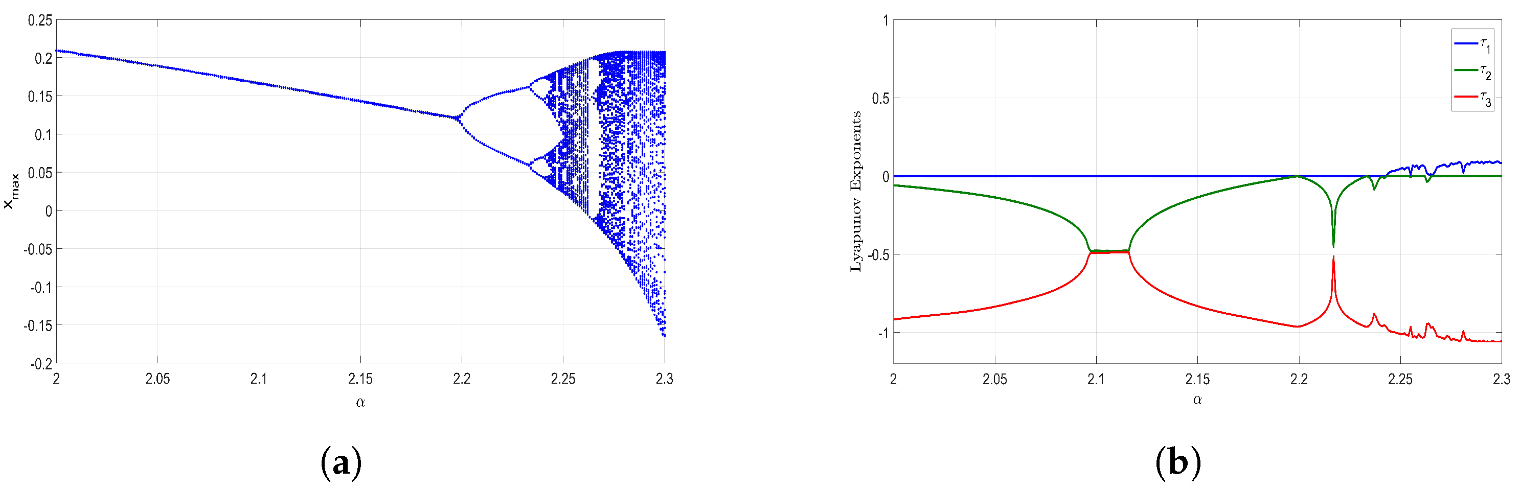
3. Bifurcation Analysis of the New Jerk System with a Stable Equilibrium
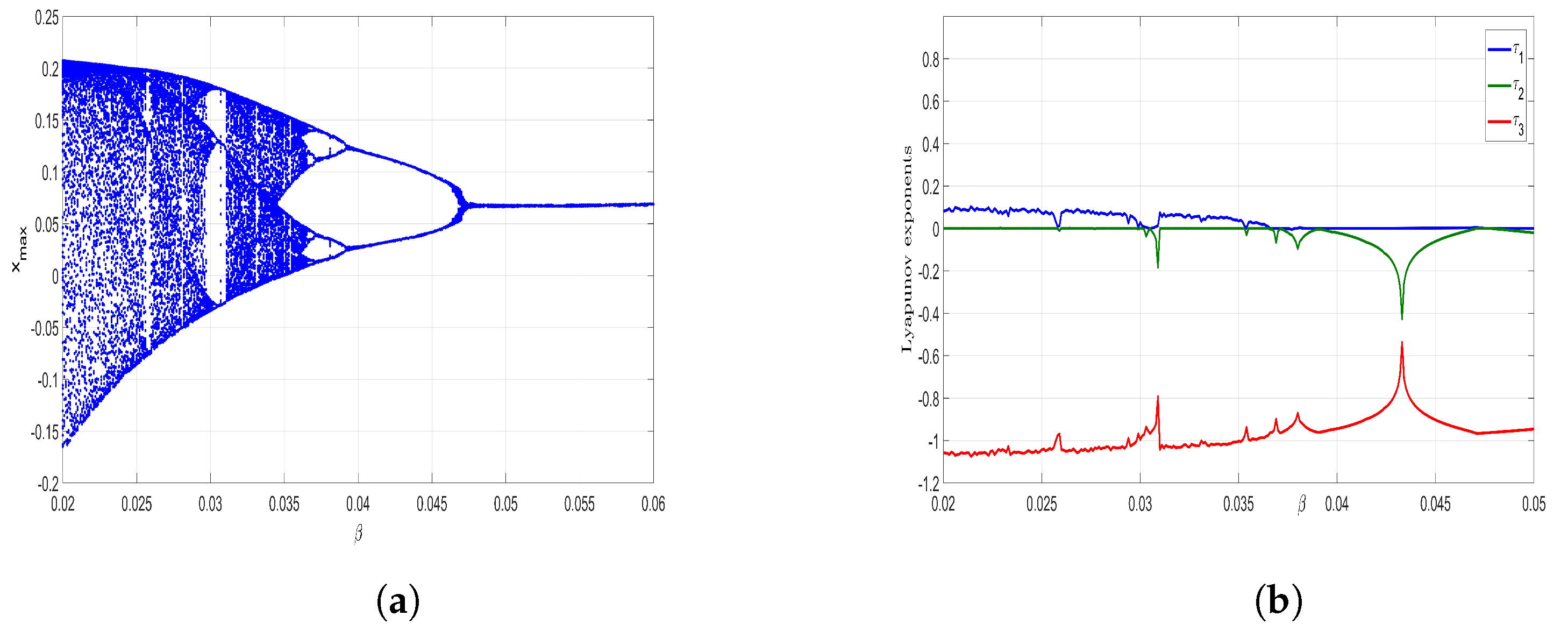
3.1. Variation with Respect to the Parameter
3.2. Variation with Respect to the Parameter
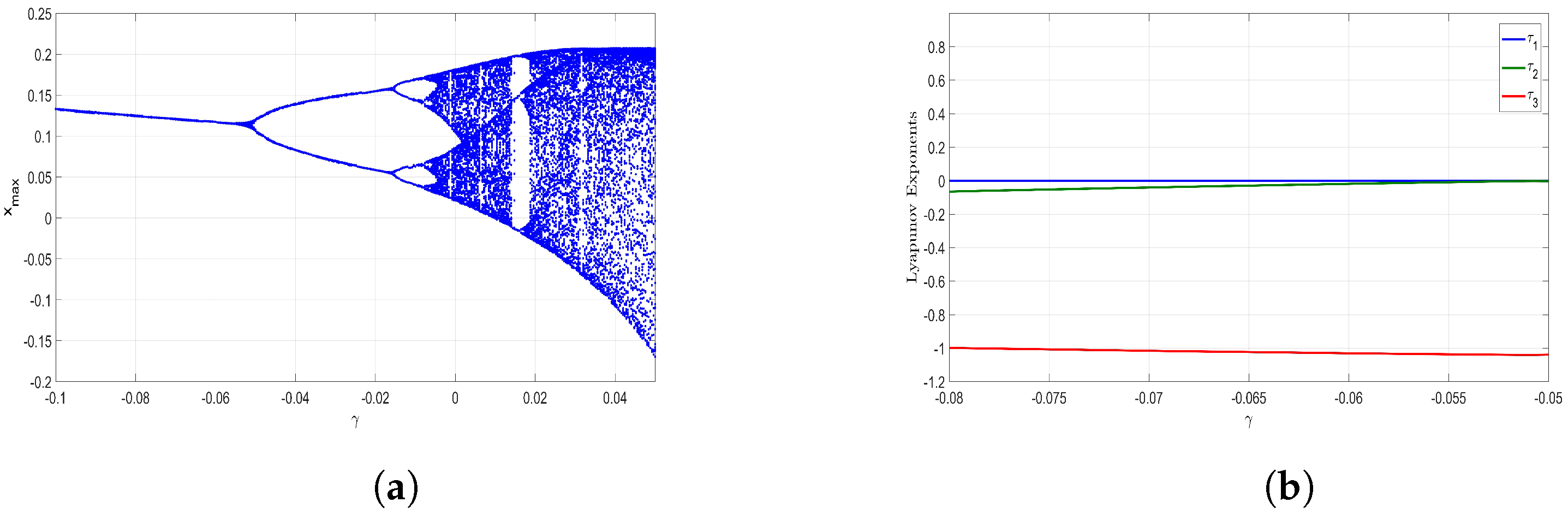
3.3. Variation with Respect to the Parameter
4. Multistability and Coexisting Attractors of the New Jerk System with a Stable Equilibrium
4.1. CASE(A): , and
4.2. CASE(B): , and
5. Complete Synchronization of the New Jerk Systems Using Backstepping Control
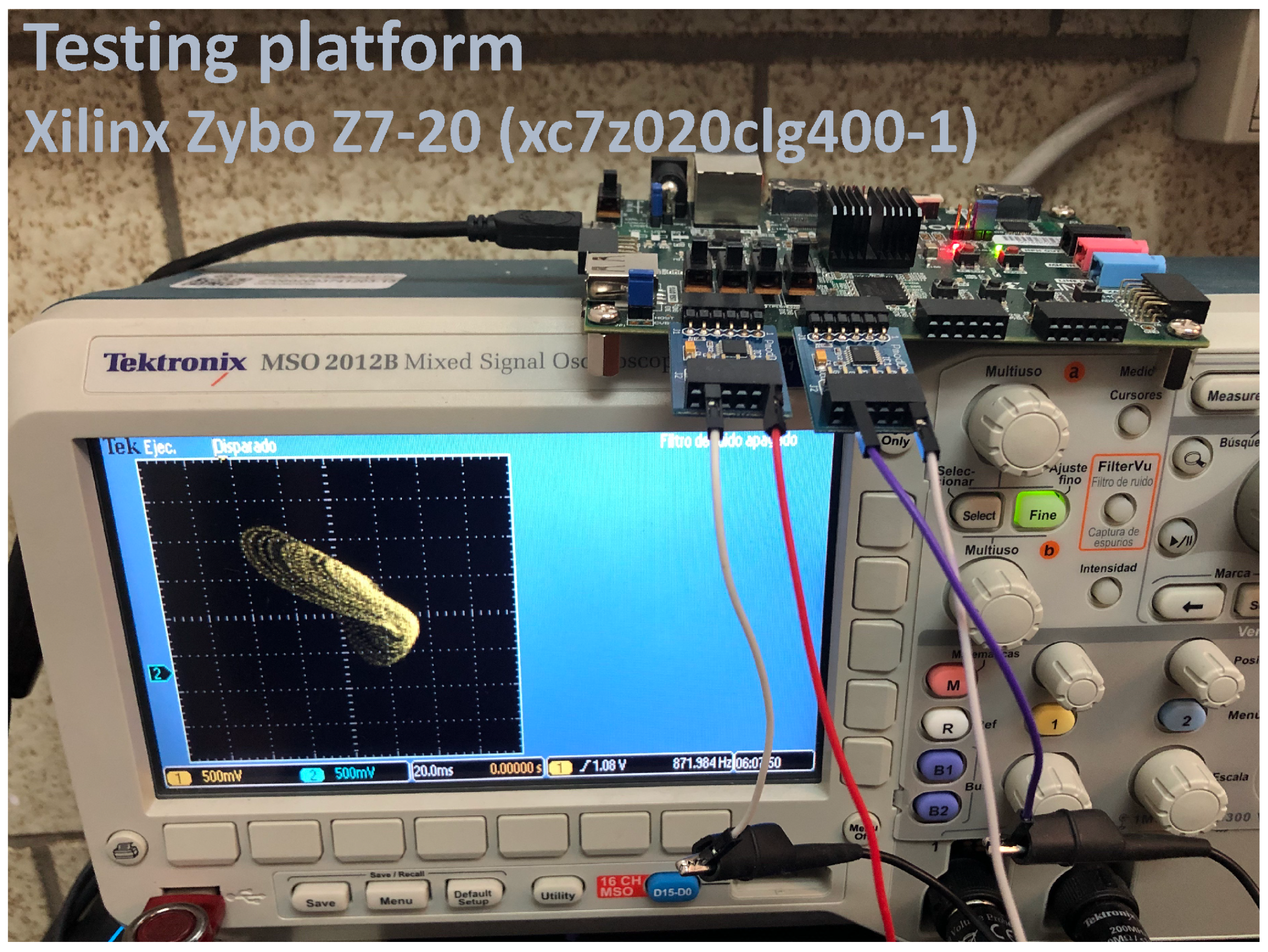
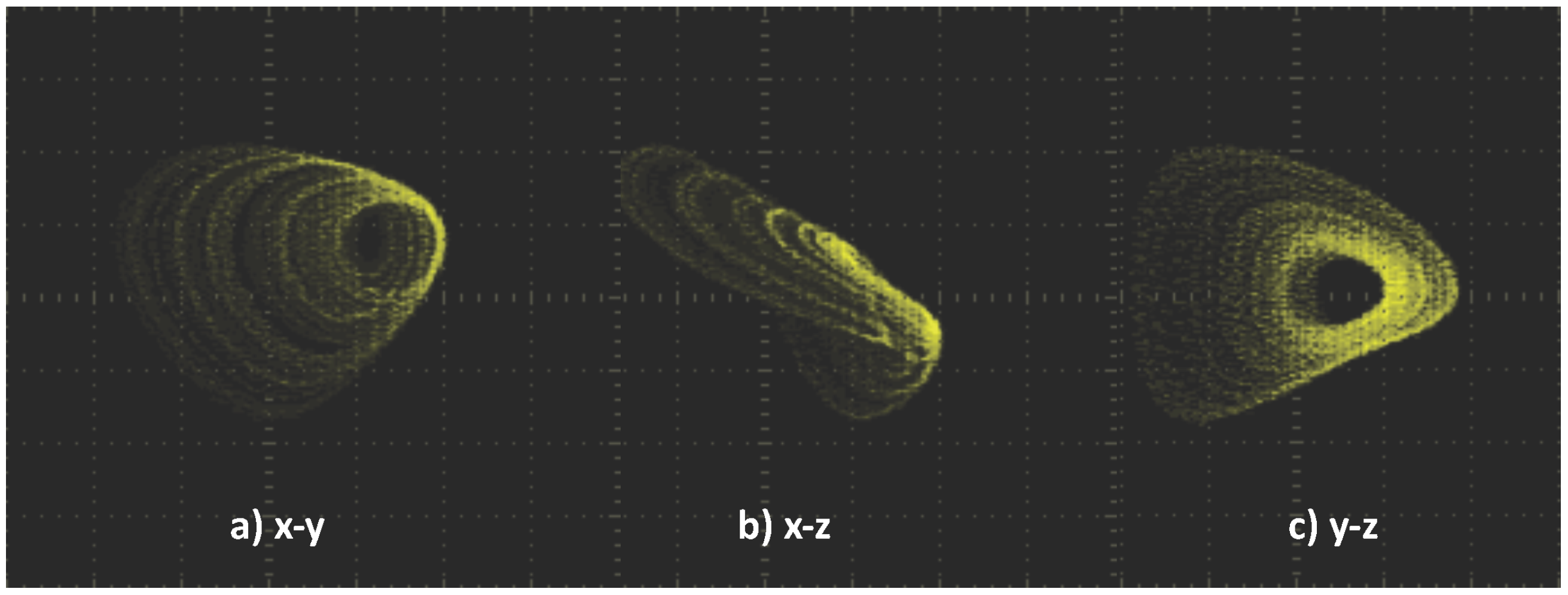
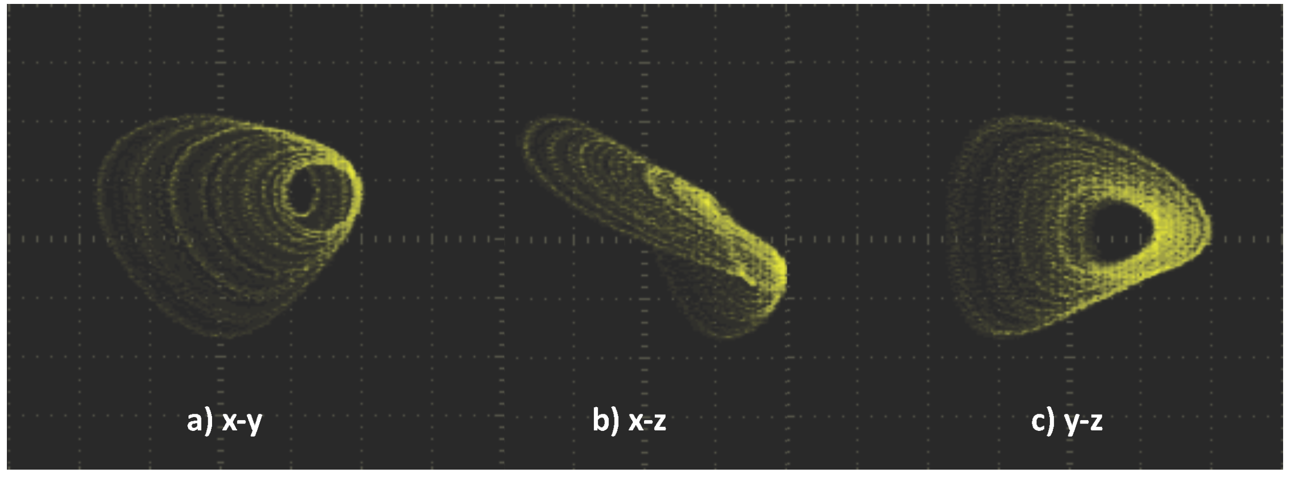
6. FPGA-Based Implementation of the New Jerk System with a Stable Equilibrium
7. Conclusions
Author Contributions
Funding
Data Availability Statement
Acknowledgments
Conflicts of Interest
References
- Shahna, K. Novel chaos based cryptosystem using four-dimensional hyper chaotic map with efficient permutation and substitution techniques. Chaos Solitons Fractals 2023, 170, 113383. [Google Scholar] [CrossRef]
- Kifouche, A.; Azzaz, M.S.; Hamouche, R.; Kocik, R. Design and implementation of a new lightweight chaos-based cryptosystem to secure IoT communications. Int. J. Inf. Secur. 2022, 21, 1247–1262. [Google Scholar] [CrossRef]
- He, J.; Qiu, W.; Cai, J. Synchronization of hyperchaotic systems based on intermittent control and its application in secure communication. J. Adv. Comput. Intell. Intell. Inform. 2023, 27, 292–303. [Google Scholar] [CrossRef]
- Gokyildirim, A.; Kocamaz, U.E.; Uyaroglu, Y.; Calgan, H. A novel five-term 3D chaotic system with cubic nonlinearity and its microcontroller-based secure communication implementation. AEU Int. J. Electron. Commun. 2023, 160, 154497. [Google Scholar] [CrossRef]
- Alshehri, M.S.; Almakdi, S.; Qathrady, M.A.; Ahmad, J. Cryptanalysis of 2D-SCMCI hyperchaotic map based image Encryption Algorithm. Comput. Syst. Sci. Eng. 2023, 46, 2401–2414. [Google Scholar] [CrossRef]
- Lin, L.; Li, Q.; Xi, X. Asynchronous secure communication scheme using a new modulation of message on optical chaos. Opt. Quantum Electron. 2023, 55, 15. [Google Scholar] [CrossRef]
- Lai, Q.; Chen, Z. Grid-scroll memristive chaotic system with application to image encryption. Chaos Solitons Fractals 2023, 170, 113341. [Google Scholar] [CrossRef]
- Li, H.; Li, C.; He, S. Locally Active Memristor with Variable Parameters and Its Oscillation Circuit. Int. J. Bifurc. Chaos 2023, 33, 2350032. [Google Scholar] [CrossRef]
- Dhivakaran, P.B.; Vinodkumar, A.; Vijay, S.; Lakshmanan, S.; Alzabut, J.; El-Nabulsi, R.A.; Anukool, W. Bipartite Synchronization of Fractional-Order Memristor-Based Coupled Delayed Neural Networks with Pinning Control. Mathematics 2022, 10, 3699. [Google Scholar] [CrossRef]
- Anbalagan, P.; Ramachandran, R.; Alzabut, J.; Hincal, E.; Niezabitowski, M. Improved Results on Finite-Time Passivity and Synchronization Problem for Fractional-Order Memristor-Based Competitive Neural Networks: Interval Matrix Approach. Fractal Fract. 2022, 6, 36. [Google Scholar] [CrossRef]
- Demirkol, A.S.; Ascoli, A.; Weiher, M.; Tetzlaff, R. Exact Inductorless Realization of Chua Circuit Using Two Active Elements. IEEE Trans. Circuits Syst. II Express Briefs 2023, 70, 1620–1624. [Google Scholar] [CrossRef]
- Yang, N.; Liu, N.; Wu, C. Non-homogeneous non-inductive chaotic circuit based on Fractional-Order Active Generalized Memristor and its FPGA implementation. Circuits Syst. Signal Process. 2023, 42, 1940–1958. [Google Scholar] [CrossRef]
- Raab, M.; Zeininger, J.; Suchorski, Y.; Tokuda, K.; Rupprechter, G. Emergence of chaos in a compartmentalized catalytic reaction nanosystem. Nat. Commun. 2023, 14, 736. [Google Scholar] [CrossRef] [PubMed]
- Kannan, K.S.; Ansari, M.A.T.; Amutha, K.; Chinnathambi, V.; Rajasekar, S. Control of chaos and bifurcation by nonfeedback methods in an autocatalytic chemical system. Int. J. Chem. Kinet. 2023, 55, 261–267. [Google Scholar] [CrossRef]
- Li, F.; Zeng, J. Multi-Scroll Attractor and Multi-Stable Dynamics of a Three-Dimensional Jerk System. Energies 2023, 16, 2494. [Google Scholar] [CrossRef]
- Dongmo, E.D.; Ramadoss, J.; Tchamda, A.R.; Sone, M.E.; Rajagopal, K. FPGA implementation, controls and synchronization of autonomous Josephson junction jerk oscillator. Phys. Scr. 2023, 98, 035224. [Google Scholar] [CrossRef]
- Qin, M.H.; Lai, Q. Extreme multistability and amplitude modulation in memristive chaotic system and application to image encryption. Optik 2023, 272, 170407. [Google Scholar] [CrossRef]
- Ramadoss, J.; Kengnou Telem, A.N.; Kengne, J.; Rajagopal, K. Complex dynamics in a novel jerk system with septic nonlinearity: Analysis, control, and circuit realization. Phys. Scr. 2023, 98, 015205. [Google Scholar] [CrossRef]
- Etemad, S.; Iqbal, I.; Samei, M.E.; Rezapour, S.; Alzabut, J.; Sudsutad, W.; Goksel, I. Some inequalities on multi-functions for applying in the fractional Caputo–Hadamard jerk inclusion system. J. Inequalities Appl. 2022, 84, 1–28. [Google Scholar] [CrossRef]
- Zhang, S.; Zeng, Y. A simple Jerk-like system without equilibrium: Asymmetric coexisting hidden attractors, bursting oscillation and double full Feigenbaum remerging trees. Chaos Solitons Fractals 2019, 120, 25–40. [Google Scholar] [CrossRef]
- Vaidyanathan, S.; Benkouider, K.; Sambas, A. A new multistable jerk chaotic system, its bifurcation analysis, backstepping control-based synchronization design and circuit simulation. Arch. Control. Sci. 2022, 32, 123–152. [Google Scholar]
- Sambas, A.; Vaidyanathan, S.; Moroz, I.M.; Idowu, B.; Mohamed, M.A.; Mamat, M.; Sanjaya, W.M. A simple multi-stable chaotic jerk system with two saddle-foci equilibrium points: Analysis, synchronization via backstepping technique and MultiSim circuit design. Int. J. Electr. Comput. Eng. 2021, 11, 2941–2952. [Google Scholar] [CrossRef]
- Vaidyanathan, S.; Moroz, I.M.; Abd El-Latif, A.A.; Abd-El-Atty, B.; Sambas, A. A new multistable jerk system with Hopf bifurcations, its electronic circuit simulation and an application to image encryption. Int. J. Comput. Appl. Technol. 2021, 67, 29–46. [Google Scholar] [CrossRef]
- Pham, V.T.; Vaidyanathan, S.; Volos, C.; Jafari, S.; Kapitaniak, T. A new multi-stable chaotic hyperjerk system, its special features, circuit realization, control and synchronization. Arch. Control. Sci. 2020, 30, 23–45. [Google Scholar]
- Vijayakumar, M.; Karthikeyan, A.; Zivcak, J.; Krejcar, O.; Namazi, H. Dynamical behavior of a new chaotic system with one stable equilibrium. Mathematics 2021, 9, 3217. [Google Scholar]
- Massimo Cencini, F.C.; Vulpiani, A. Chaos: From Simple Models to Complex Systems; World Scientific: Singapore, 2010. [Google Scholar]
- Dingwell, J.B. Lyapunov Exponents. In Wiley Encyclopedia of Biomedical Engineering; Akay, M., Ed.; Wiley: Toronto, ON, Canada, 2006; pp. 1–12. [Google Scholar]
- Chen, Z.M. A note on Kaplan-Yorke-type estimates on the fractal dimension of chaotic attractors. Chaos Solitons Fractals 1993, 3, 575–582. [Google Scholar] [CrossRef]
- Li, B.; Zhang, Y.; Li, X.; Eskandari, Z.; He, Q. Bifurcation analysis and complex dynamics of a Kopel triopoly model. J. Comput. Appl. Math. 2023, 426, 115089. [Google Scholar] [CrossRef]
- Qiu, H.; Xu, X.; Jiang, Z.; Sun, K.; Cao, C. Dynamical behaviors, circuit design, and synchronization of a novel symmetric chaotic system with coexisting attractors. Sci. Rep. 2023, 13, 1893. [Google Scholar] [CrossRef]
- Yan, H.; Qiao, Y.; Ren, Z.; Duan, L.; Miao, J. Master–slave synchronization of fractional-order memristive MAM neural networks with parameter disturbances and mixed delays. Commun. Nonlinear Sci. Numer. Simul. 2023, 120, 107152. [Google Scholar] [CrossRef]
- Kumar, S.; Prasad, R.P.; Nishad, C.; Tiwary, A.K.; Khan, F. Analysis and chaos synchronization of Genesio–Tesi system applying sliding mode control techniques. Int. J. Dyn. Control. 2023, 11, 656–665. [Google Scholar] [CrossRef]
- Dousseh, Y.P.; Monwanou, A.V.; Koukpémèdji, A.A.; Miwadinou, C.H.; Chabi Orou, J.B. Dynamics analysis, adaptive control, synchronization and anti-synchronization of a novel modified chaotic financial system. Int. J. Dyn. Control. 2023, 11, 862–876. [Google Scholar] [CrossRef]
- Ouannas, A.; Azar, A.T.; Vaidyanathan, S. On a simple approach for Q-S synchronisation of chaotic dynamical systems in continuous-time. Int. J. Comput. Sci. Math. 2017, 8, 20–27. [Google Scholar] [CrossRef]
- Benkouider, K.; Vaidyanathan, S.; Sambas, A.; Tlelo-Cuautle, E.; Abd El-Latif, A.A.; Abd-El-Atty, B.; Bermudez-Marquez, C.F.; Sulaiman, I.M.; Awwal, A.M.; Kumam, P. A New 5-D Multistable Hyperchaotic System with Three Positive Lyapunov Exponents: Bifurcation Analysis, Circuit Design, FPGA Realization and Image Encryption. IEEE Access 2022, 10, 90111–90132. [Google Scholar] [CrossRef]
- Hua, Z.; Zhou, B.; Zhou, Y. Sine-transform-based chaotic system with FPGA implementation. IEEE Trans. Ind. Electron. 2017, 65, 2557–2566. [Google Scholar] [CrossRef]
- Guillén-Fernández, O.; Moreno-López, M.F.; Tlelo-Cuautle, E. Issues on applying one-and multi-step numerical methods to chaotic oscillators for FPGA implementation. Mathematics 2021, 9, 151. [Google Scholar] [CrossRef]
- Yang, G.; Zhang, X.; Moshayedi, A.J. Implementation of the Simple Hyperchaotic Memristor Circuit with Attractor Evolution and Large-Scale Parameter Permission. Entropy 2023, 25, 203. [Google Scholar] [CrossRef]
- de la Fraga, L.G.; Ovilla-Martínez, B. A chaotic PRNG tested with the heuristic Differential Evolution. Integration 2023, 90, 22–26. [Google Scholar] [CrossRef]
- Wolf, A.; Swift, J.B.; Swinney, H.L.; Vastano, J.A. Determining Lyapunov exponents from a time series. Phys. D Nonlinear Phenom. 1985, 16, 285–317. [Google Scholar] [CrossRef] [Green Version]
- Dong, C. Dynamic Analysis of a Novel 3D Chaotic System with Hidden and Coexisting Attractors: Offset Boosting, Synchronization, and Circuit Realization. Fractal Fract. 2022, 6, 547. [Google Scholar] [CrossRef]
- Li, C.; MIn, F.; Jin, Q.; Ma, H. Extreme multistability analysis of memristor-based chaotic system and its application in image decryption. AIP Adv. 2017, 7, 125204. [Google Scholar] [CrossRef] [Green Version]
- Vaidyanathan, S.; Azar, A.T. Backstepping Control of Nonlinear Dynamical Systems; Academic Press: New York, NY, USA, 2021. [Google Scholar]
- Dong, H.; Cao, J.; Liu, H. Observers-based event-triggered adaptive fuzzy backstepping synchronization of uncertain fractional order chaotic systems. Chaos 2023, 33, A366. [Google Scholar] [CrossRef] [PubMed]
- Yan, S.; Wang, J.; Wang, E.; Wang, Q.; Sun, X.; Li, L. A four-dimensional chaotic system with coexisting attractors and its backstepping control and synchronization. Integration 2023, 91, 67–78. [Google Scholar] [CrossRef]
- Gong, X.; Wang, H.; Ji, Y.; Zhang, Y. Optical chaos generation and synchronization in secure communication with electro-optic coupling mutual injection. Opt. Commun. 2022, 521, 128565. [Google Scholar] [CrossRef]


| Jerk System | Case | MLE | Kaplan-Yorke Dimension |
|---|---|---|---|
| Vijayakumar Jerk system (8) | Case A | ||
| New Jerk system (17) | Case A | ||
| Vijayakumar Jerk system (8) | Case B | ||
| New Jerk system (17) | Case B |
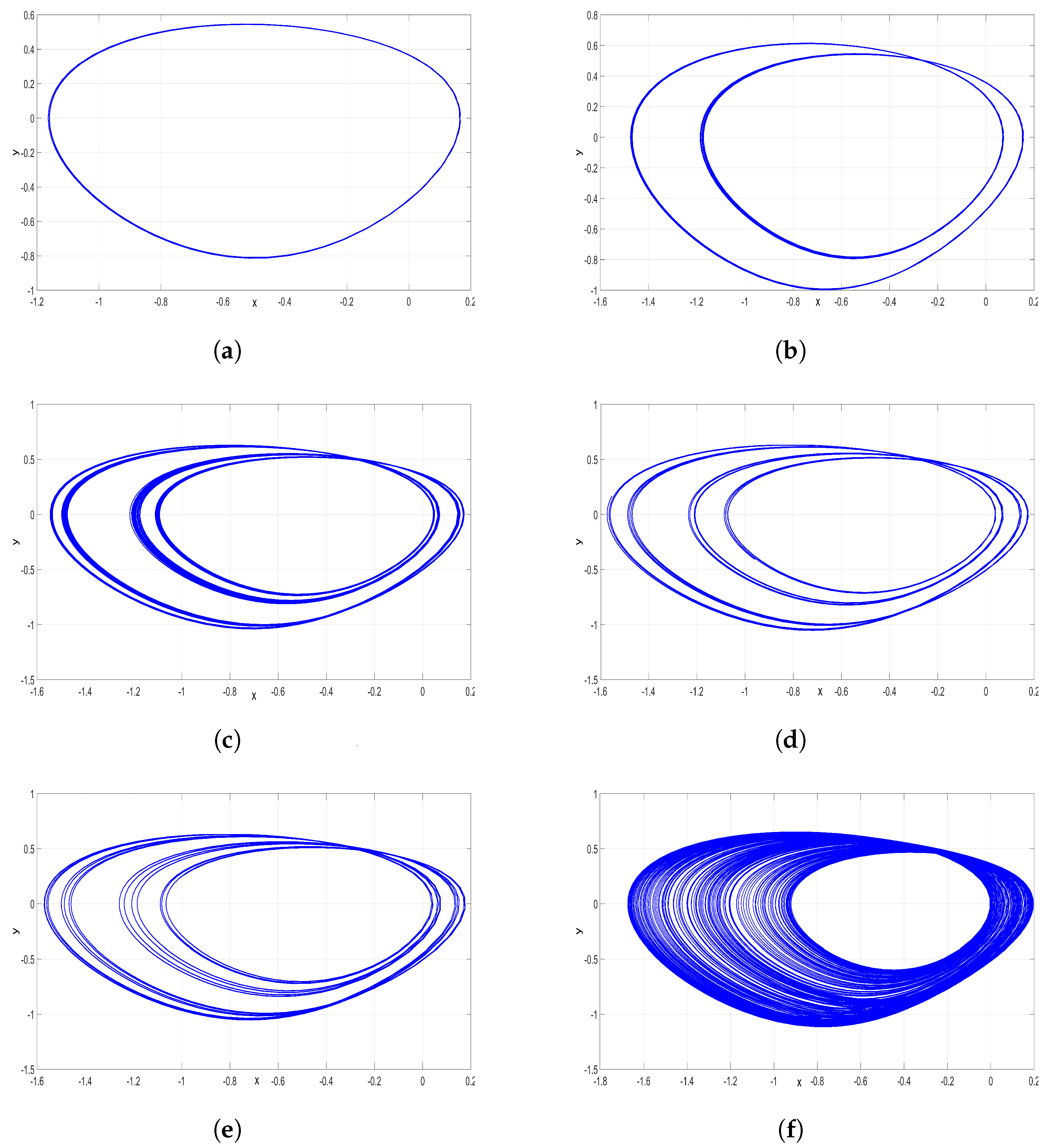
| Range | Value | Dynamics | Attractor |
|---|---|---|---|
| 2.1 | Period-1 | Figure 8a | |
| 2.22 | Period-2 | Figure 8b | |
| 2.236 | Period-4 | Figure 8c | |
| 2.2412 | Period-8 | Figure 8d | |
| 2.2424 | Period-16 | Figure 8e | |
| 2.2465 | Chaos | Figure 8f |
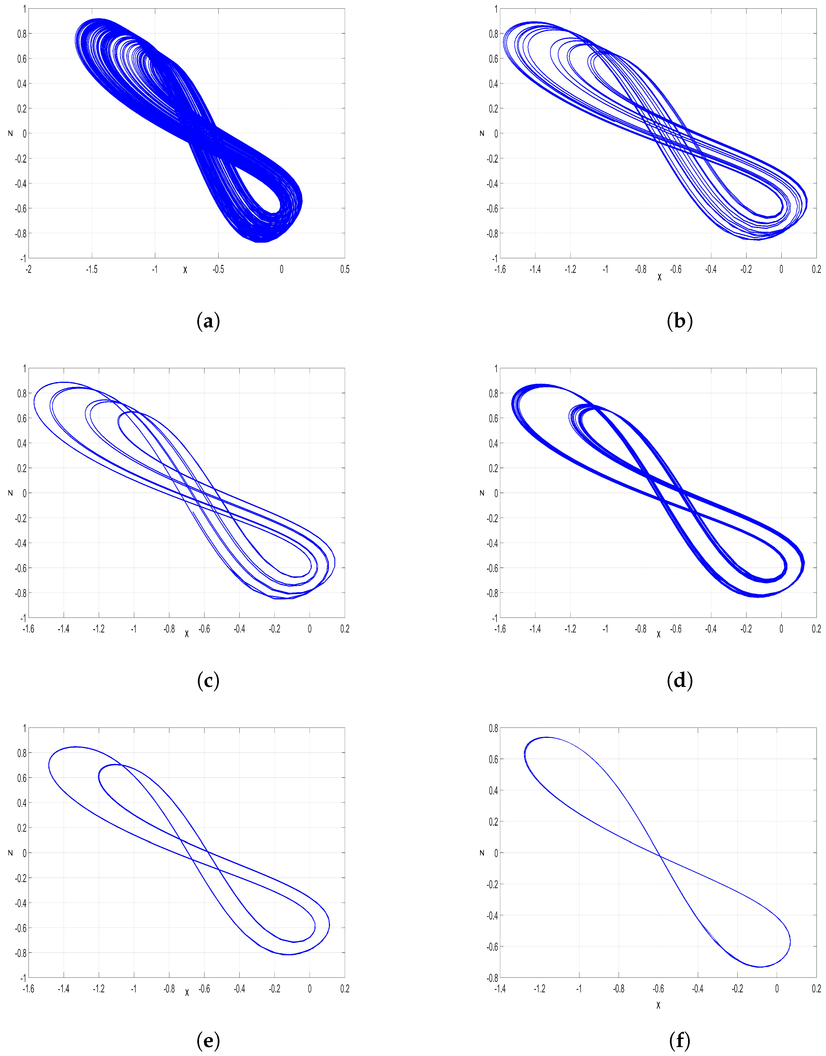
| Range | Value | Dynamics | Attractor |
|---|---|---|---|
| Chaos | Figure 10a | ||
| Period-16 | Figure 10b | ||
| Period-8 | Figure 10c | ||
| Period-4 | Figure 10d | ||
| Period-2 | Figure 10e | ||
| Period-1 | Figure 10f |
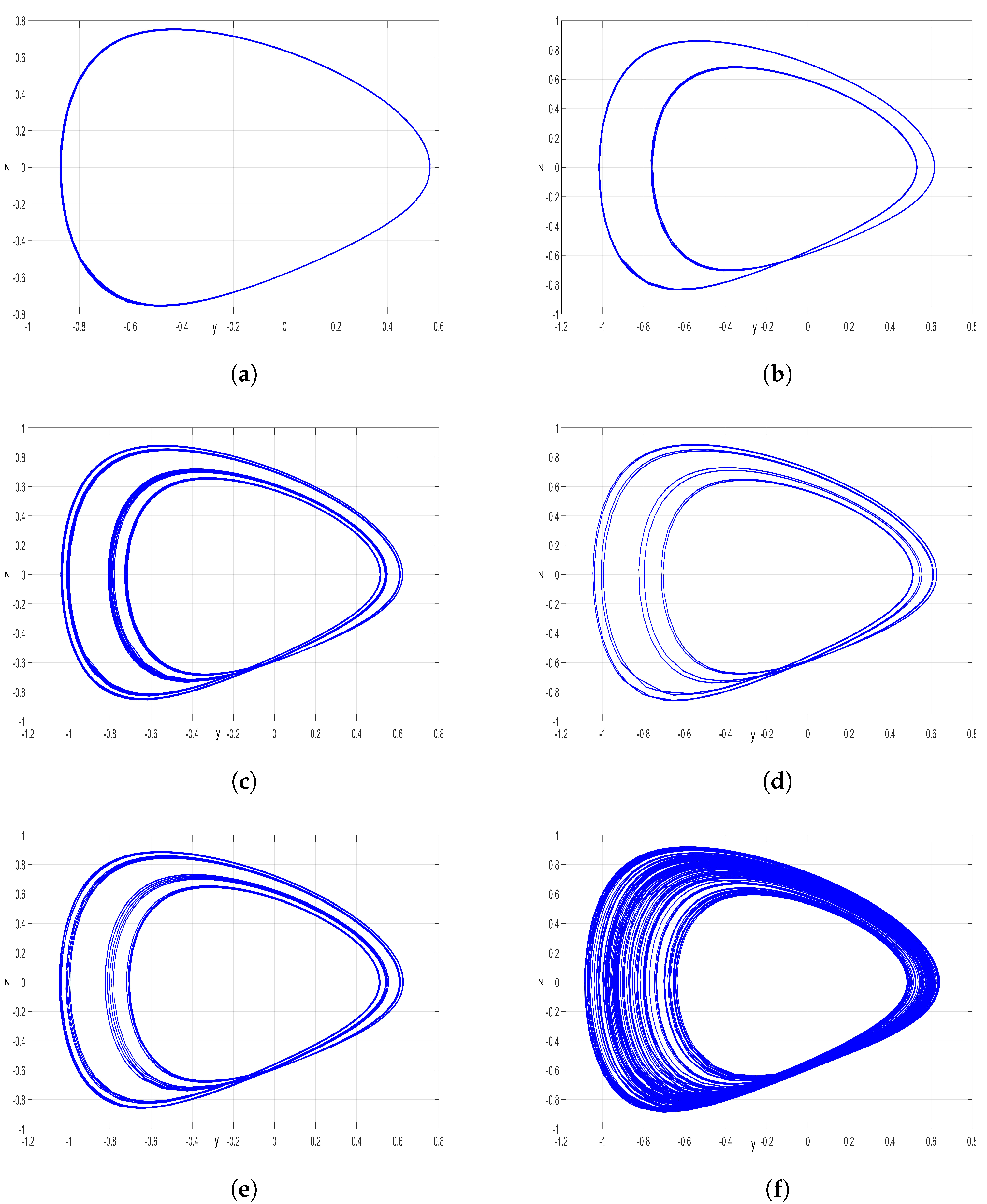
| Range | Value | Dynamics | Attractor |
|---|---|---|---|
| 2.1 | Period-1 | Figure 12a | |
| 2.22 | Period-2 | Figure 12b | |
| 2.236 | Period-4 | Figure 12c | |
| 2.2412 | Period-8 | Figure 12d | |
| 2.2424 | Period-16 | Figure 12e | |
| 2.2465 | Chaos | Figure 12f |
| Resources | Used | Util |
|---|---|---|
| Slice | 134 | 1.01% |
| LUTs | 302 | 0.57% |
| FFs | 192 | 0.17% |
| DSPs | 16 | 5.18% |
| Frequency Max | 123 MHz | - |
Disclaimer/Publisher’s Note: The statements, opinions and data contained in all publications are solely those of the individual author(s) and contributor(s) and not of MDPI and/or the editor(s). MDPI and/or the editor(s) disclaim responsibility for any injury to people or property resulting from any ideas, methods, instructions or products referred to in the content. |
© 2023 by the authors. Licensee MDPI, Basel, Switzerland. This article is an open access article distributed under the terms and conditions of the Creative Commons Attribution (CC BY) license (https://creativecommons.org/licenses/by/4.0/).
Share and Cite
Vaidyanathan, S.; Azar, A.T.; Hameed, I.A.; Benkouider, K.; Tlelo-Cuautle, E.; Ovilla-Martinez, B.; Lien, C.-H.; Sambas, A. Bifurcation Analysis, Synchronization and FPGA Implementation of a New 3-D Jerk System with a Stable Equilibrium. Mathematics 2023, 11, 2623. https://doi.org/10.3390/math11122623
Vaidyanathan S, Azar AT, Hameed IA, Benkouider K, Tlelo-Cuautle E, Ovilla-Martinez B, Lien C-H, Sambas A. Bifurcation Analysis, Synchronization and FPGA Implementation of a New 3-D Jerk System with a Stable Equilibrium. Mathematics. 2023; 11(12):2623. https://doi.org/10.3390/math11122623
Chicago/Turabian StyleVaidyanathan, Sundarapandian, Ahmad Taher Azar, Ibrahim A. Hameed, Khaled Benkouider, Esteban Tlelo-Cuautle, Brisbane Ovilla-Martinez, Chang-Hua Lien, and Aceng Sambas. 2023. "Bifurcation Analysis, Synchronization and FPGA Implementation of a New 3-D Jerk System with a Stable Equilibrium" Mathematics 11, no. 12: 2623. https://doi.org/10.3390/math11122623