Chaos Synchronization of Two Györgyi–Field Systems for the Belousov–Zhabotinsky Chemical Reaction

Abstract

Chemical reactions with oscillating behavior can present a chaos state in specific conditions. In this study, we analyzed the dynamic of the chaotic Belousov–Zhabotinsky (BZ) reaction using the Györgyi–Field model in order to identify the conditions of the chaos behavior. We studied the behavior of the reaction under different parameters that included both a low and high flux of chemical species. We performed our analysis of the flow regime in the conditions of an open reaction system, as this provides information about the behavior of the reaction over time. The proposed method for determining the favorable conditions for obtaining the state of chaos is based on the time evolution of the intermediate species and phase portraits. The synchronization of two Györgyi–Field systems based on the adaptive feedback method of control is presented in this work. The transient time until synchronization depends on the initial conditions of the two systems and on the strength of the controllers. Among the areas of interest for possible applications of the control method described in this paper, we can include identification of the reaction parameters and the extension to the other chaotic systems.

1. Introduction

The Belousov–Zhabotinsky (BZ) reaction is the prototype system for nonlinear chemical dynamics. Initially, the reaction was discovered accidentally by the Soviet chemist Boris Pavlovich Belousov in the 1950s, who mixed bromate, citric acid and cerium ions [1]. Zhabotinsky [2] visually highlighted the oscillation of concentration of the chemical species by replacing citric acid with malonic acid in Belousov reaction. The red-blue visual effect and cycle period are given by the nature of a catalyst. The cycle period can be increased by using ferroin as a catalyst, which acts as a perturbator on frequency, and by changing the pH of medium which perturbs the cycle’s magnitude and direction [3].

The BZ reaction is famous because it passes through multiple intermediary stages, which can be considered metastable states. In the early 1970s, Field, Körös and Noyes [4] (FKN) used combined kinetic and thermodynamic approaches to propose a detailed mechanism capable of describing the oscillatory reactions by using 11 main reactions and 12 chemical species. Later, in 1974, Field and Noyes [5] reduced the FKN model to a simpler, realistic model described by few metastable reactions—the model known as Oregonator. After that, Györgyi, Rempe and Field [6] developed a new model that relied on 11 dynamic variables and 19 reactions to explain the chaos in the BZ reaction.

Currently, it is generally accepted that chemical systems can exhibit chaotic behavior, which is very important for chemical processes and biological structures. The control of these phenomena has a great practical impact, even though it is very difficult to do; this is the reason why theoretical models are useful in these situations. In addition, information about the control of these models can provide insight into the self-control of biological structures where the behavior of the dynamic systems is performed by a feedback mechanism.

The oscillation states of the BZ reaction can be experimentally controlled by monitoring the continuous flow in reaction tanks [7]. The spatiotemporal pattern of these oscillations can be simulated by using the dynamics of the coupled map lattice [7] or Brusselator equation [8,9]. Over the last decades, there has been considerable progress in generalizing the concept of synchronization to include the case of clusters [10], neuron networks [11] and chaotic oscillators networks [12], especially from technical reasons [13,14,15]. Many examples of synchronizations have been documented in the literature, as a current, theoretical understanding of the phenomena behind experimental studies is needed [12,13,14,15,16,17,18,19,20,21,22,23,24,25,26]. The main aim of this paper is to study the synchronization of two chemical chaotic systems based on the adaptive feedback method of control by considering one of the famous ideal chemical models, named Györgyi–Field [27], which explains the chaotic behavior of the Belousov–Zhabotinsky chemical reaction.

In the next section, we present the model and method used for obtaining an efficient mechanism that describes both behaviors of the dynamic systems, oscillatory and chaotic, especially for the BZ reactions. The results obtained for two cases of the input reaction are presented and discussed in the third section. We determined the conditions under which the reaction can be controlled in order to obtain different behaviors using two input concentrations. Additionally, a new adaptive method for the synchronization of two dynamic Györgyi–Field systems is proposed.

2. Models and Methods

Dynamic chemical systems depend on the environmental conditions and initial concentrations of species. There reactions can be explained by using the mathematical models and parameters which are determined by using the synchronization method.

2.1. Györgyi–Field Model

In this paper, we used a mathematical model, developed in 1992, by Györgyi and Field [27] to describe the BZ reaction, which exhibits chaotic behavior in specific conditions, using differential equations. The model considered that the reaction takes place in a continuous-flow stirred-tank reactor and has the advantage that the intermediate species of BZ chemical reactions are reduced at three (x, v, z).

The GF model represents the evolution of specific chemical reactions in an open system and its mechanism consists of the following (1)–(7) elementary steps [27,28]:

$$\mathrm{X}+\mathrm{Y}+\mathrm{H}\stackrel{k_1}{\to }2\mathrm{V}$$

(1)

$$\mathrm{Y}+\mathrm{A}+2\mathrm{H}\stackrel{k_2}{\to }\mathrm{V}+\mathrm{X}$$

(2)

$$2\mathrm{X}\stackrel{k_3}{\to }\mathrm{V}$$

(3)

$$1/2\mathrm{X}+\mathrm{A}+\mathrm{H}\stackrel{k_4}{\to }\mathrm{X}+\mathrm{Z}$$

(4)

$$\mathrm{X}+\mathrm{Z}\stackrel{k_5}{\to }1/2\mathrm{X}$$

(5)

$$\mathrm{V}+\mathrm{Z}\stackrel{k_6}{\to }\mathrm{Y}$$

(6)

$$\mathrm{Z}+\mathrm{M}\stackrel{k_7}{\to }?$$

(7)

In the GF model, the reactants are ions or molecules whose concentrations change in time. The mathematical variables of the GF model represent the following chemical species: X = [HBrO₂], Y = [Br⁻] şi Z = [Ce⁴⁺], A = [BrO₃⁻], H = [H⁺], M = [CH₂(COOH)₂], V = BrCH(COOH)₂ [29].

The evolution of the intermediate species in time is described by a nonlinear system of Equation (8), in which C play the role of a catalyst. In this reaction, the catalyst is represented by the total concentration of Ce ions in the system (C = [Ce]).

The nonlinear system is described by the following differential equations:

$$\begin{gathered} \frac{dx}{d\tau }={\mathrm{T}}_0[-k_1{\mathrm{HY}}_{0}x\overline{y}+k_2{\mathrm{AH}}^2{\mathrm{Y}}_0{\mathrm{X}}_0^{-1}\overline{y}-2k_3{\mathrm{X}}_0{x}^2+1/2k_4{\mathrm{A}}^{\frac{1}{2}}{\mathrm{H}}^{\frac{3}{2}}{\mathrm{X}}_0^{-\frac{1}{2}}· \\ ·\left(\mathrm{C}-{\mathrm{Z}}_{0}z\right)x^{\frac{1}{2}}-1/2k_5{\mathrm{Z}}_{0}xz-k_{f}x] \\ \frac{dz}{d\tau }={\mathrm{T}}_0\left[k_4{\mathrm{A}}^{\frac{1}{2}}{\mathrm{H}}^{\frac{3}{2}}{\mathrm{X}}_0^{\frac{1}{2}}·\left(\frac{\mathrm{C}}{{\mathrm{Z}}_0}-z\right)x^{\frac{1}{2}}-k_5{\mathrm{X}}_{0}xz-\alpha k_6{\mathrm{V}}_{0}zv-\beta k_7\mathrm{M}z-k_{f}z\right] \\ \frac{dv}{d\tau }={\mathrm{T}}_0\left[2k_1{\mathrm{HX}}_0{\mathrm{Y}}_0{\mathrm{V}}_0^{-1}x\overline{y}+k_2{\mathrm{AH}}^2{\mathrm{Y}}_0{\mathrm{V}}_0^{-1}\overline{y}+k_3{\mathrm{X}}_0^2{\mathrm{V}}_0^{-1}{x}^2-\alpha k_6{\mathrm{Z}}_{0}zv-k_{f}v\right] \end{gathered}$$

(8)

where

$$\begin{gathered} \overline{y }=\left[\left(\alpha k_6{\mathrm{Z}}_0{\mathrm{V}}_{0}zv\right)/\left(k_1{\mathrm{HX}}_{0}x+k_2{\mathrm{AH}}^2+k_f\right)\right]/{\mathrm{Y}}_0; {\mathrm{T}}_0=1/\left(10k_2\mathrm{AHC}\right) \\ {\mathrm{X}}_0=k_2{\mathrm{AH}}^2/k_5; {\mathrm{Y}}_0=4k_2{\mathrm{AH}}^2/k_5; {\mathrm{Z}}_0=\mathrm{CA}/40\mathrm{M}; {\mathrm{V}}_0=4\mathrm{AHC}/{\mathrm{M}}^2; \\ \tau =t/{\mathrm{T}}_0;x=\mathrm{X}/{\mathrm{X}}_0; z=\mathrm{Z}/{\mathrm{Z}}_0 \mathrm{and} v=\mathrm{V}/{\mathrm{V}}_0. \end{gathered}$$

(9)

For simplicity, the terms were normalized (Equation (9)), where τ is the term of normalization for the time t, and x, v, z correspond to the intermediate chemical species in the reaction.

2.2. Numerical Calculations

The numerical calculations were performed using ordinary differential equations implemented in the ODE45 solver from MATLAB^®, developed by The MathWorks Inc., Natick, MA, USA. The ODE45 solver was used to solve first-order equations for time dependence due to good accuracy for the present study.

The initial conditions used in numerical calculations were chosen so that the concentrations of intermediate species sustain the chemical reactions.

2.3. The Synchronizations

The synchronization of two systems is one of the most studied topics in chaos and it is used in physical, chemical, biological, social and engineering dynamic systems [7,8,15]. Theoretical methods of synchronization are very difficult to develop but are necessary for controlling the evolution of systems. Until now, numerous models of synchronization were proposed to describe chemical reactions, biological systems, electrical circuits and networks [12,13,14,15,16,17,18,19,20,21,22,23,24,25,26].

To synchronize two identical chemical systems, we followed an adaptive-feedback method [22,25,26] based on the Lyapunov–Lasalle theory. For synchronization, in this method, a driver system is considered in the following form:

$$\frac{dy}{d\tau }=f\left(y\right)+z\left(y-x\right)$$

(10)

where

$$z\left(y-x\right)={\displaystyle \sum }_{i=1}^n{z}_{\mathrm{i}}{e}_{\mathrm{i}}$$

with

$$e_i=\left(y_{\mathrm{i}}-x_{\mathrm{i}}\right)$$

The coupling will be determined by the equation:

$$\frac{dz}{dt}=-{\displaystyle {\mathsf{\Upsilon }}_i}{\left(y_{\mathrm{i}}-x_{\mathrm{i}}\right)}^2=-{\displaystyle {\mathsf{\Upsilon }}_i}{e}_i{}^2$$

(11)

The objective of the synchronization is:

$$\underset{\tau \to \infty }{\lim }\parallel e\left(\tau \right)\parallel \to 0$$

(12)

The model is based on a master and slave systems, respectively, on controllers (ϒ). The values of the controllers were chosen so that the fastest synchronization is obtained. A faster synchronization relies on choosing adequate values for ϒ and for the initial concentrations. According to this method, the master system of the Györgyi–Field mechanism is described by Equation (8), and the slaves are described by:

$$\begin{array}{c}\frac{d{x}_1}{d\tau }={\mathrm{T}}_0[-k_1{\mathrm{HY}}_0{x}_1\overline{y}+k_2{\mathrm{AH}}^2{\mathrm{Y}}_0{\mathrm{X}}_0^{-1}\overline{y}-2k_3{\mathrm{X}}_0{x}_1{}^2+1/2k_4{\mathrm{A}}^{1/2}{\mathrm{H}}^{3/2}{\mathrm{X}}_0^{-1/2}·\hfill \\ \left(\mathrm{C}-{\mathrm{Z}}_0{z}_1\right)x^{1/2}-1/2k_5{\mathrm{Z}}_0{x}_1{z}_1-k_f{x}_1]+x_2\left(x_1-x\right)\hfill \\ \frac{d{z}_1}{d\tau }={\mathrm{T}}_0[k_4{\mathrm{A}}^{1/2}{\mathrm{H}}^{3/2}{\mathrm{X}}_0^{1/2}·\left(\mathrm{C}/{\mathrm{Z}}_0-z_1\right)x_1{}^{1/2}-k_5{\mathrm{X}}_0{x}_1{z}_1-\alpha k_6{\mathrm{V}}_0{z}_1{v}_1-\hfill \\ -\beta k_7\mathrm{M}{z}_1-k_f{z}_1]+z_2\left(z_1-z\right)\hfill \\ \frac{d{v}_1}{d\tau }={\mathrm{T}}_0[2k_1{\mathrm{HX}}_0{\mathrm{Y}}_0{\mathrm{V}}_0^{-1}{x}_1\overline{y}+k_2{\mathrm{AH}}^2{\mathrm{Y}}_0{\mathrm{V}}_0^{-1}\overline{y}+k_3{\mathrm{X}}_0^2{\mathrm{V}}_0^{-1}{x}_1{}^2-\hfill \\ \hfill -\alpha k_6{\mathrm{Z}}_0{z}_1{v}_1-k_f{v}_1]+v_2\left(v_1-v\right).\end{array}$$

(13)

The control strengths used for synchronization is defined by:

$$\begin{gathered} \frac{d{x}_2}{d\tau }=-{(x_1-x)}^2 \\ \frac{d{z}_2}{d\tau }=-{(z_1-z)}^2 \\ \frac{d{v}_2}{d\tau }=-{(v_1-v)}^2 \end{gathered}$$

(14)

The method is simpler and more efficient than other methods used for the synchronizations of chemical reactions and avoids constructing the Lyapunov–Lasalle functions [22]. The method is not faster than techniques based on symmetry and synchronization coefficients [24], but, in our case, the present model was the only one that gave adequate results for the analyzed time intervals.

3. Results and Discussion

We considered that the chemical reaction take place in an open system in which we can control the flow of chemical compounds. We studied the evolution of the reaction according to the flow rate in order to identify the conditions when the reaction presents chaotic and oscillatory behavior.

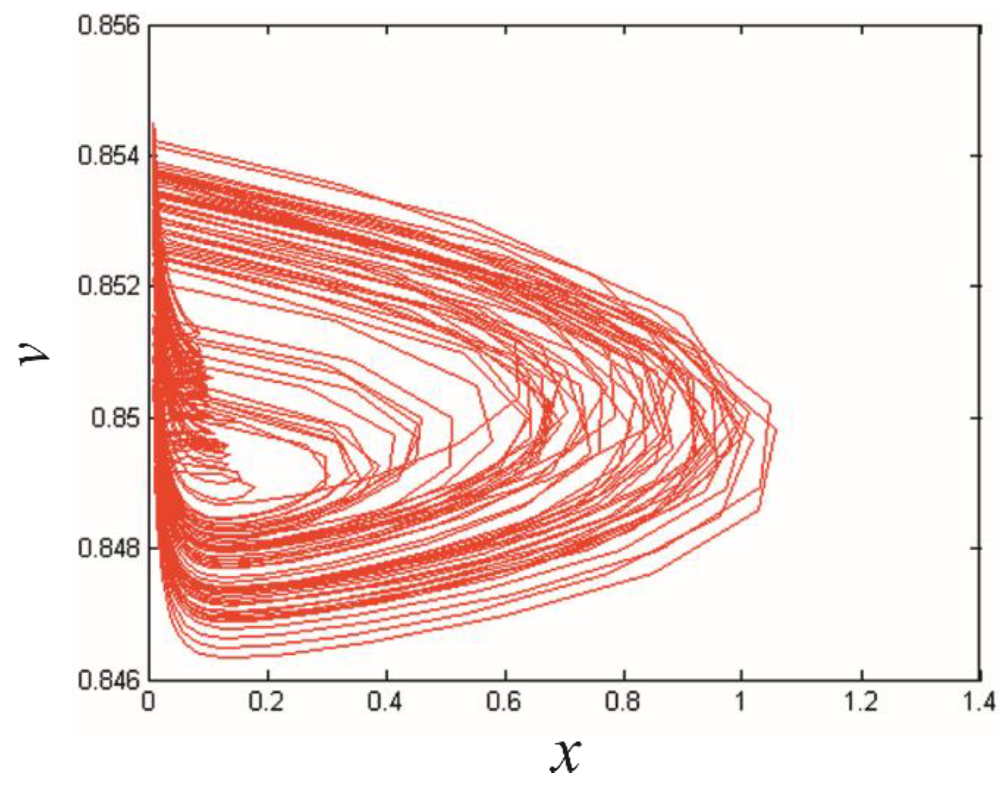
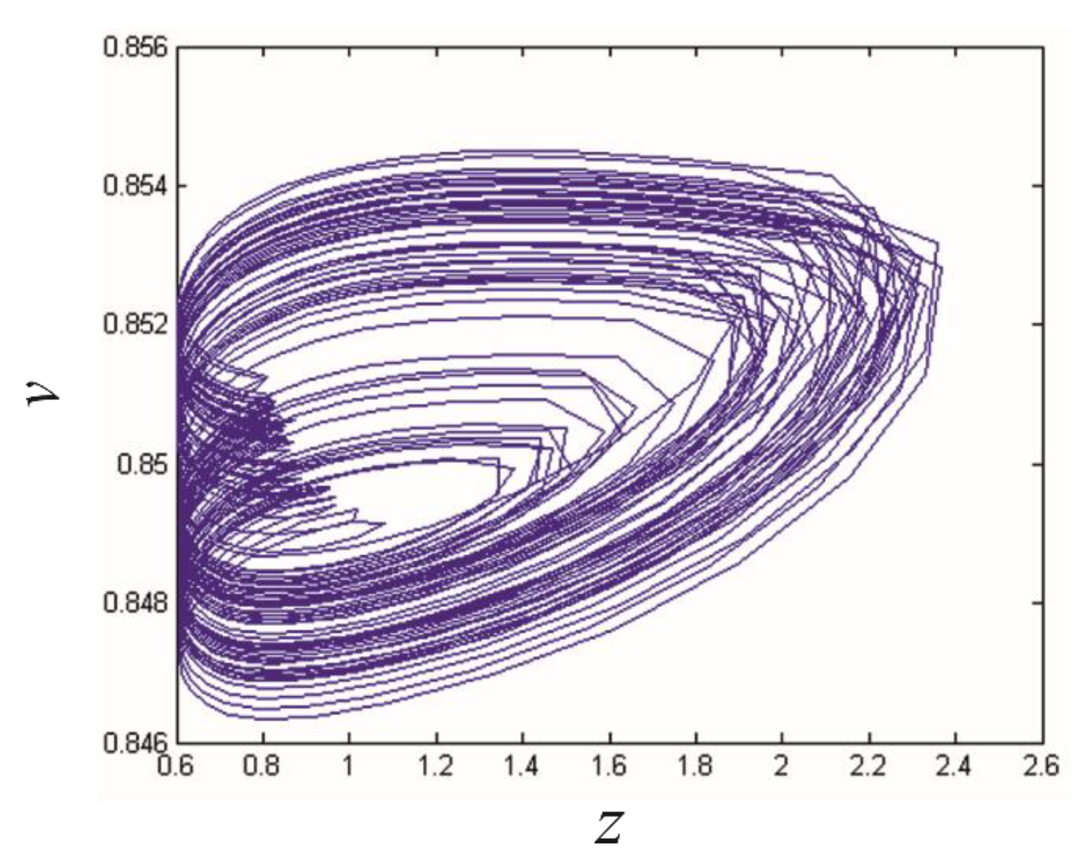
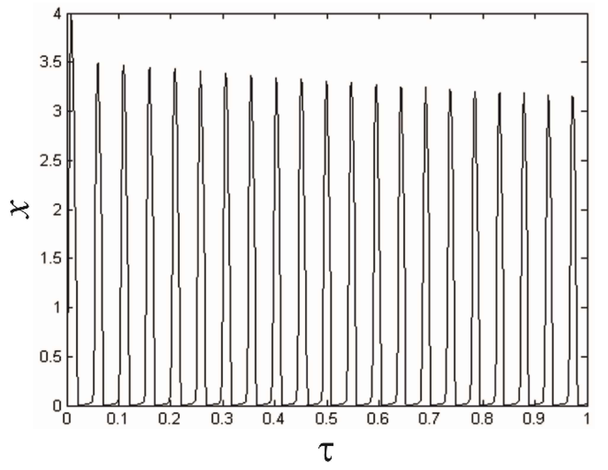
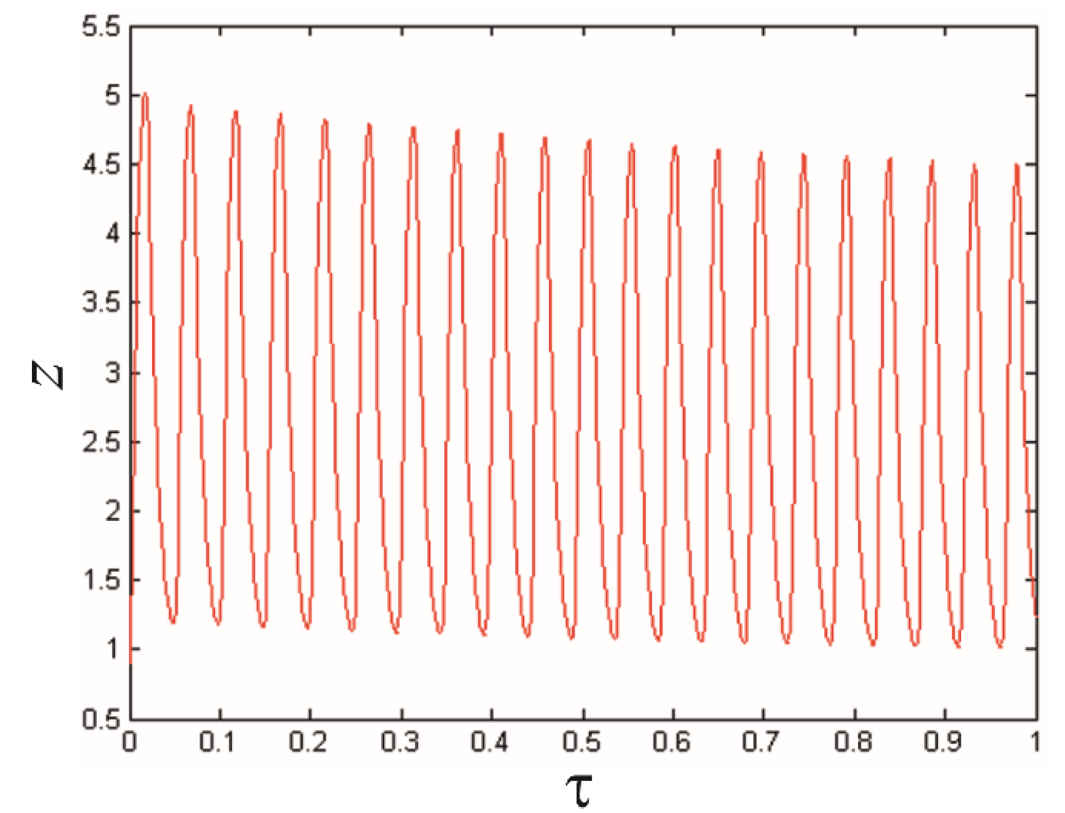
3.1. Behavior of the System at Different Input Concentrations

Initially, in this type of reaction, oscillatory behavior was observed [4], but later, it was demonstrated that in some specific conditions, the experimental reaction deviates from this characteristic to chaotic behavior [6,27]. We proposed to determine possible experimental conditions when the reaction would become chaotic based on analyzing two cases. We presumed that the flow of chemicals’ input influences output behavior. To demonstrate this hypothesis, we considered two identical systems with very different input concentration values.

3.1.1. Low Flux Input

Our simulations show that the BZ reaction presents chaotic behavior if the concentrations of chemical species and the values of reaction parameters fulfill certain conditions. In nonlinear dynamical systems, the initial conditions are important because they completely change the course of the reaction [30]. First, we considered a low flux for the dynamic Györgyi–Field system with the reaction values, as shown in

Table 1. The concentrations of intermediate species and the values of reaction parameters in the GF model for chaotic behavior at low flux.

Chemical Intermediate Species	Concentration	Reaction Parameters in GF Model	Value	Reaction Parameters in GF Model	Value
A	0.1 mol	α	666.67	k3	3000 mol−1 s−1
M	0.25 mol	β	0.3478	k4	55.2 mol−2.5 s−1;
H	0.26 mol	kf	3.9 × 10−4	k5	7000 mol−1 s−1;
C	8.33·10−4 mol	k1	4 × 106 mol−1 s−1	k6	0.09 mol−1 s−1
		k2	2 mol−3 s−1	k7	0.23 mol−1 s−1

.

The time variations of the intermediate species were obtained using the following initial values: x(0) = 0.045 (Figure 1); z(0) = 0.9 (Figure 2) and v(0) = 0.85 (Figure 3).

The evolution of the concentrations of intermediate species can exhibit a simple or complex periodic behavior and, in some situations, it can become chaotic (Figure 1, Figure 2 and Figure 3). For small values of the k_f parameter, the concentration of x(τ) shows a simple periodic oscillation. This behavior changes into a periodic oscillation with different numbers of peaks by increasing the value of the k_f, and chaotic behavior is obtained for k_f = 3.9 × 10⁻⁴. After this stage, the oscillating behavior with multiple peaks is resumed.

In systems with multi-metastable stages, the phase trajectory of the attractors depends on the initial conditions [31]. For specific conditions at low flux (Table 1), the bidimensional attractors are open cycles where the portraits of the phases do not overlap (Figure 4, Figure 5 and Figure 6), which confirms the hypothesis that the system has a chaotic behavior.

3.1.2. High Flux Input

The simulations for high flux were performed for the parameters listed in

Table 2. The concentrations of intermediate species and the values of reaction parameters in GF model for oscillatory behavior at high flux.

Chemical Intermediary Species	Concentration	Reaction Parameters in GF Model	Value	Reaction Parameters in GF Model	Value
A	0.14 mol	α	333.33	k3	3000 mol−1 s−1
M	0.3 mol	β	0.2609	k4	55.2 mol−2.5 s−1
H	0.26 mol	kf	6.18 × 10−4	k5	7000 mol−1 s−1
C	0.001 mol	k1	4 × 106 mol−1 s−1	k6	0.09 mol−1 s−1
		k2	2 mol−3 s−1	k7	0.23 mol−1 s−1

to evaluate if the chaotic state will be reached. Increasing the flow rate (Table 2) in the reaction tank, for the same initial values of variables previously observed, lead to the oscillatory behaviors from Figure 7, Figure 8, Figure 9 and Figure 10.

For a high flow in the open reaction system, the concentrations of all intermediate species and parameter values listed in Table 2 presented oscillatory behaviors (Figure 6, Figure 7 and Figure 8) in time (τ). The amplitudes of the oscillations are high and decrease for the x and y species in time, instead the concentration of v have a small variation which increase during the process (Figure 9). For researchers, the variation of the concentrations of the intermediate species is important tools for determining the experimental conditions of reaction.

At the beginning, the trajectories of bidimensional and three-dimensional attractors exhibit large open cycles that shrink until they become stabile closed cycles (Figure 10, Figure 11 and Figure 12). The trajectories obtained in the GF model indicate the pure oscillatory behavior of BZ reaction (Figure 10, Figure 11 and Figure 12), in which the amplitudes and frequencies of oscillations the depend by time [32] and temperature [33].

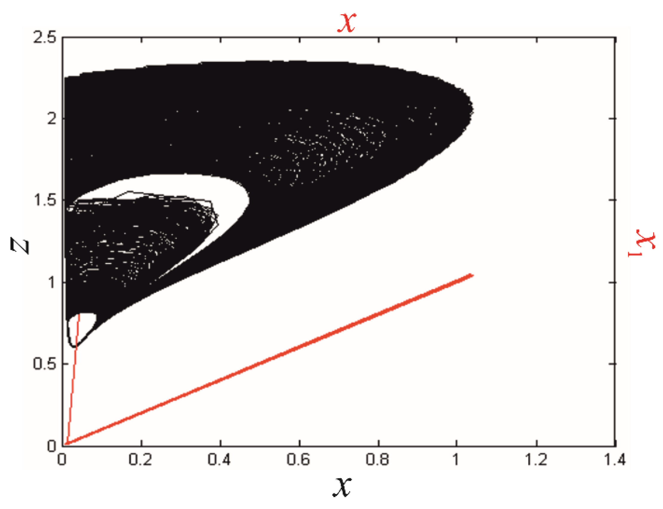
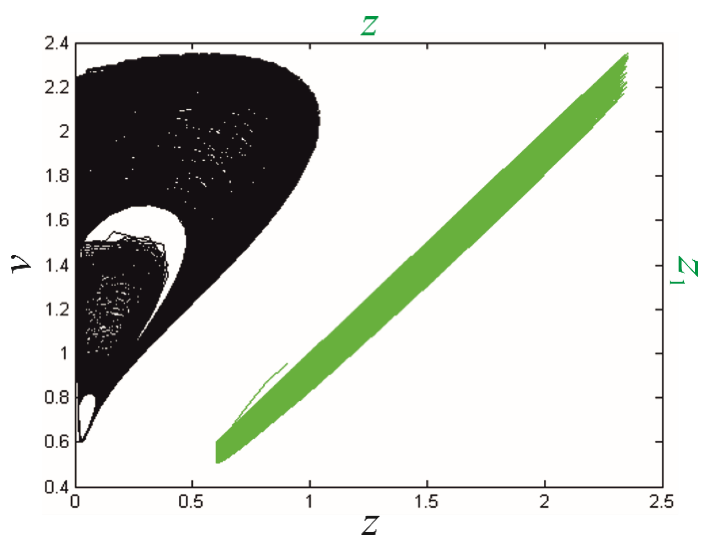
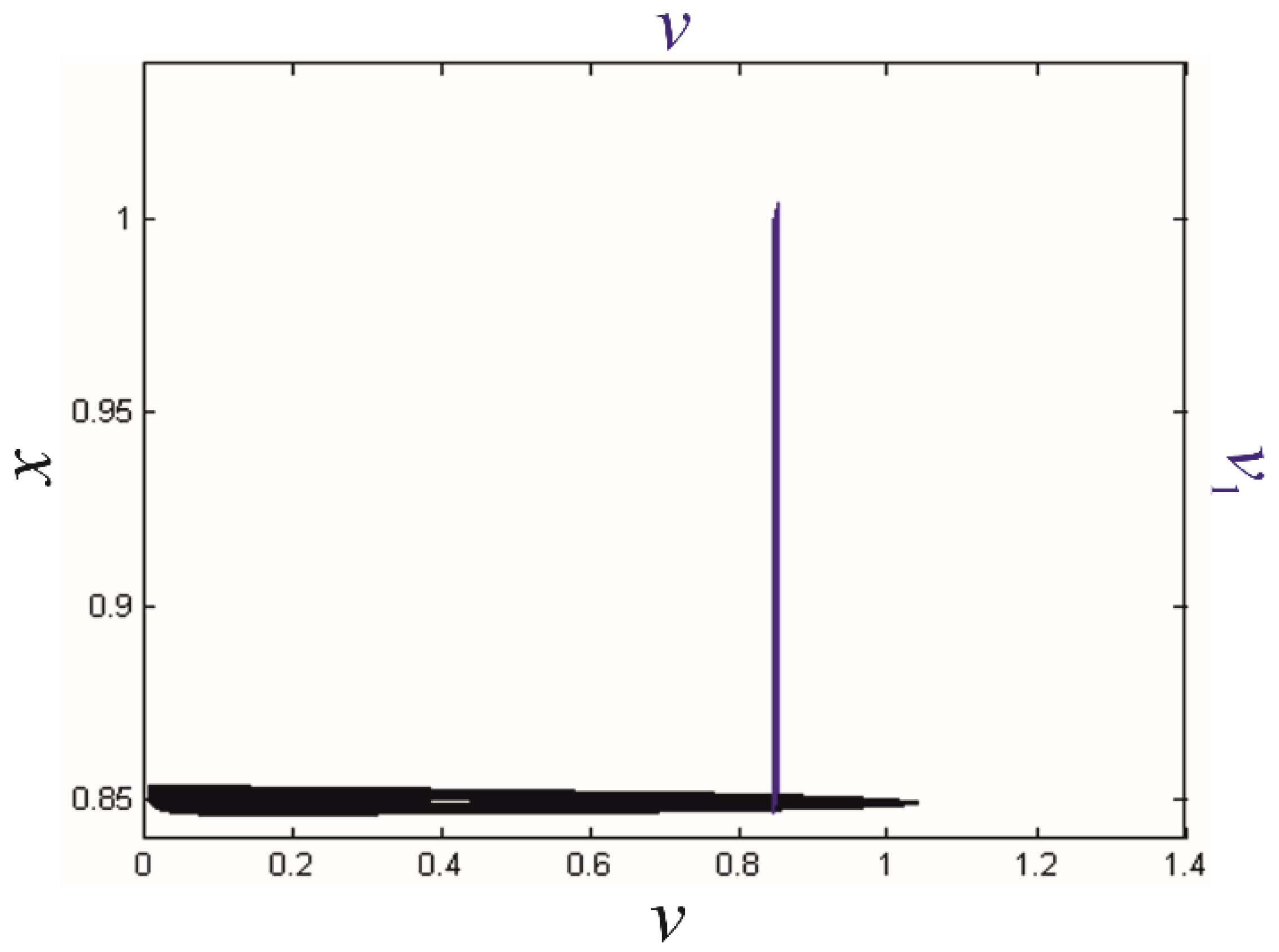
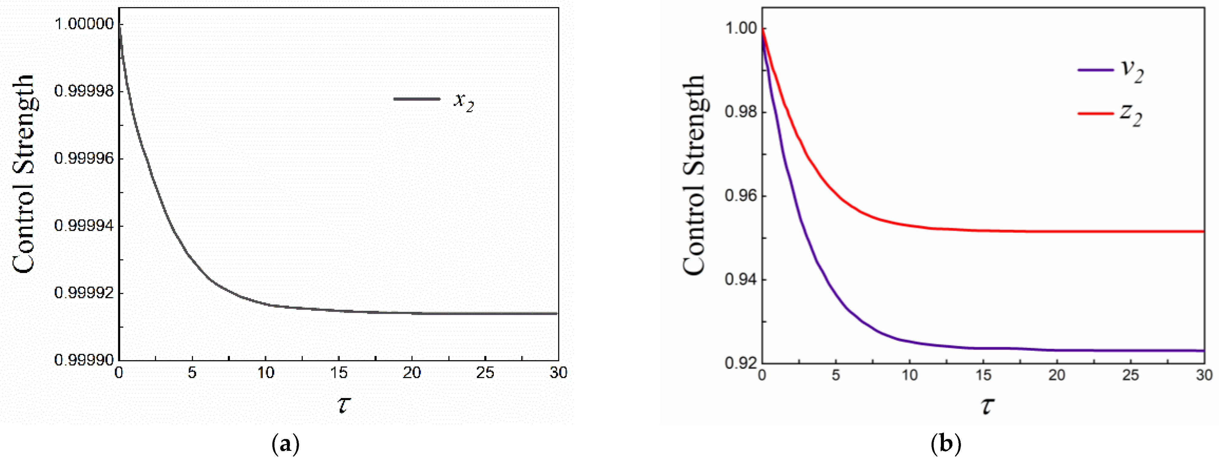
3.2. Synchronization of Two Györgyi–Field Systems

The proposed method can be used to determine the synchronization time for the two identical systems. In time, the differences between masters and slaves reduce to zero (Figure 13), demonstrating the synchronization of the two Györgyi–Field systems. The value of normalized time variable (τ) is almost the same value (τ = 25) in all cases (Figure 13).

Comparing the phase portraits of masters [(x, z), (z, v), (v, x)] and the phase portraits of master–slave systems [(x, x₁), (z, z₁), (v, v₁)] we observe that the last phase portraits become straight lines (Figure 14, Figure 15 and Figure 16), which is proof that synchronization is achieved.

Figure 17a,b show that the values of controllers became constants in time further proof that synchronization is achieved.

4. Conclusions

In this study, we analyzed the Belousov–Zhabotinsky chemical reaction using two dynamic Györgyi–Field systems which can offer information about the behavior of the reaction in time. The results highlighted that in specific reaction conditions at a low flow of chemical compounds through the reaction tank a chaotic state can be obtained, whereas for high flow only an oscillatory behavior can be achieved. The method used for synchronization of the two Györgyi–Field systems based on controllers has the advantage that can be easily applied for this type of systems and can also be extended to the other chemical reactions or biological structures with oscillatory behavior.

The synchronization technique is not the fastest method but for the GF model it proved to be a relatively simple and effective method.

At continuous high flux, the cycle periods of oscillations (τ = 0.0476) and the synchronization periods for all control strengths (τ = 25) are the same for all intermediate species. These denote that the reaction conditions are met. The transient time until synchronization depends on initial conditions of the two systems, the concentrations of chemical compounds from reaction tank and on the strength of the controllers.

Establishing the initial conditions, the concentrations of the chemical species and the synchronization parameters is necessary to achieve the control of chaotic behavior in future experiments.

References

1. Sagues, F.; Epstein, I. Nonlinear chemical dynamics. Dalton Trans. 2003, 7, 1201–1217. [Google Scholar] [CrossRef]
2. Zhabotinsky, A.M. A history of chemical oscillations and waves. Chaos Interdiscip. J. Nonlinear Sci. 1991, 1, 379–386. [Google Scholar] [CrossRef] [PubMed]
3. Horvath, V.; Epstein, I.R. Pulse-coupled Belousov-Zhabotinsky oscillators with frequency modulation. Chaos 2018, 28, 045108. [Google Scholar] [CrossRef] [PubMed]
4. Field, R.J.; Koros, E.; Noyes, R.M. Oscillations in chemical systems. II. Thorough analysis of temporal oscillation in bromate-cerium-malonic acid system. J. Am. Chem. Soc. 1972, 94, 8649–8664. [Google Scholar] [CrossRef]
5. Field, R.J.; Noyes, R.M. Oscillations in chemical systems. IV. Limit cycle behavior in a model of a real chemical reaction. J. Chem. Phys. 1974, 60, 1877. [Google Scholar] [CrossRef] [Green Version]
6. Györgyi, L.; Rempe, S.L.; Field, R.J. A novel model for the simulation of chaos in low-flow-rate experiments with the Belousov-Zhabotinsky reaction: A chemical mechanism for two-frequency oscillations. J. Phys. Chem. 1991, 95, 3159–3165. [Google Scholar] [CrossRef]
7. Yoshimoto, M.; Kurosawa, S. Pattern dynamics in the Belousov-Zhabotinsky coupled map lattice. Indian J. Phys. 2022, 96, 1489–1500. [Google Scholar] [CrossRef]
8. Kopets, E.; Karimov, A.I.; Khafizova, A.M.; Katser, E.A.; Shchetinina, T.G. Simulation of Chemical Oscillator Network. In Proceedings of the Conference of Russian Young Researchers in Electrical and Electronic Engineering (ElConRus), St. Petersburg, Russia, 25–28 January 2022; pp. 704–707. [Google Scholar] [CrossRef]
9. Kopets, E.; Tatiana, S.; Rybin, V.; Dautov, A.; Karimov, T.; Karimov, A. Simulation of a Small-Scale Chemical Reservoir Computer for Pattern Recognition. In Proceedings of the 11th Mediterranean Conference on Embedded Computing (MECO), Budva, Montenegro, 7–10 June 2022; pp. 1–4. [Google Scholar] [CrossRef]
10. Li, Y.; Lu, J.; Alofi, A.S.; Lou, J. Impulsive cluster synchronization for complex dynamical networks with packet loss and parameters mismatch. Appl. Math. Model. 2022, 112, 215–223. [Google Scholar] [CrossRef]
11. Bao, H.; Zhang, Y.; Liu, W.; Bao, B. Memristor synapse-coupled memristive neuron network: Synchronization transition and occurrence of chimera. Nonlinear Dyn. 2022, 100, 937–950. [Google Scholar] [CrossRef]
12. Shepelev, I.A.; Vadivasova, T.E. Synchronization in multiplex networks of chaotic oscillators with frequency mismatch. Chao Solitons Fractals 2021, 147, 110882. [Google Scholar] [CrossRef]
13. Eroglu, D.; Lamb, J.S.W.; Pereira, T. Synchronisation of chaos and its applications. Contemp. Phys. 2017, 58, 207–243. [Google Scholar] [CrossRef]
14. Wang, C.C.; Su, J. A new adaptive variable structure control for chaotic synchronization and secure communication. Chaos Solitons Fractals 2004, 20, 967–977. [Google Scholar] [CrossRef]
15. Vaseghi, B.; Pourmina, M.A.; Mobayen, S. Finite-time chaos synchronization and its application in wireless sensor networks. Trans. Inst. Meas. Control 2018, 40, 3788–3799. [Google Scholar] [CrossRef]
16. Chen, G.; Dong, X. From Chaos to Order: Methodologies, Perspectives and Applications; Series A; World Scientific Series on Nonlinear Science: Singapore, 1998; Volume 24. [Google Scholar] [CrossRef]
17. Grosu, I. Robust Synchronization. Phys. Rev. E 1997, 56, 3709–3712. [Google Scholar] [CrossRef]
18. Lerescu, A.I.; Constandache, N.; Oancea, S.; Grosu, I. Collection of master-slave synchronized chaotic systems. Chaos Solitons Fractals 2004, 22, 599–604. [Google Scholar] [CrossRef] [Green Version]
19. Lerescu, A.I.; Oancea, S.; Grosu, I. Collection of mutually synchronized chaotic systems. Phys. Lett. A 2006, 352, 222–228. [Google Scholar] [CrossRef] [Green Version]
20. Oancea, S.; Grosu, F.; Lazar, A.; Grosu, I. Master–slave synchronization of Lorenz systems using a single controller. Chaos Solitons Fractals 2009, 41, 2575–2580. [Google Scholar] [CrossRef]
21. Oancea, S.; Grosu, I.; Oancea, A.V. Synchronization and antisynchronization for dissipative chaotic flows. J. Adv. Res. Phys. 2010, 1, 021009. [Google Scholar]
22. Bodale, I.; Oancea, A.V. Chaos control for Willamowski-Rössler model of chemical reactions. Chaos Solitons Fractals 2015, 78, 1–9. [Google Scholar] [CrossRef]
23. Lei, A.; Ji, L.; Xu, W. Delayed feedback control of a chemical chaotic model. Appl. Math. Model. 2009, 33, 677–682. [Google Scholar] [CrossRef]
24. Rybin, V.; Tutueva, A.; Karimov, T.; Kolev, G.; Butusov, D.; Rodionova, E. Optimizing the Synchronization Parameters in Adaptive Models of Rössler system. In Proceedings of the 10th Mediterranean Conference on Embedded Computing (MECO), Budva, Montenegro, 7–10 June 2021; pp. 1–4. [Google Scholar] [CrossRef]
25. Huang, D. Simple adaptive-feedback controller for identical chaos synchronization. Phys. Rev. E 2005, 71, 037203. [Google Scholar] [CrossRef] [Green Version]
26. Guo, W.; Chen, S.; Zhou, H. A simple adaptive-feedback controller for chaos Synchronization. Chaos Solitons Fractals 2009, 39, 316–321. [Google Scholar] [CrossRef]
27. Györgyi, L.; Field, R.J. A three-variable model of deterministic chaos in the Belousov-Zhabotinsky reaction. Nature 1992, 355, 808–810. [Google Scholar] [CrossRef]
28. Zhang, D.; Gyorgyi, L.; Peltier, W.R. Deterministic chaos in the Belousov-Zhabotinsky reaction: Experiments and simulations. Chaos Interdiscip. J. Nonlinear Sci. 1993, 3, 723–745. [Google Scholar] [CrossRef]
29. Nagyová, J.B.; Jansík, B.; Lampart, M. Detection of embedded dynamics in the Györgyi-Field model. Sci. Rep. 2020, 10, 21030. [Google Scholar] [CrossRef]
30. Bao, H.; Ding, R.; Hua, M.; Wu, H.; Chen, B. Initial-Condition Effects on a Two-Memristor-Based Jerk System. Mathematics 2022, 10, 411. [Google Scholar] [CrossRef]
31. Chen, B.; Cheng, X.; Bao, H.; Chen, M.; Xu, Q. Extreme Multistability and Its Incremental Integral Reconstruction in a Non-Autonomous Memcapacitive Oscillator. Mathematics 2022, 10, 754. [Google Scholar] [CrossRef]
32. Cassani, A.; Monteverde, A.; Piumetti, M. Belousov-Zhabotinsky type reactions: The non-linear behavior of chemical systems. J. Math. Chem. 2021, 59, 792–826. [Google Scholar] [CrossRef]
33. Kabziński, J.; Mosiołek, P. Adaptive, Observer-Based Synchronization of Different Chaotic Systems. Appl. Sci. 2022, 12, 3394. [Google Scholar] [CrossRef]
Figure 1. The evolution of the x(τ) concentration at low flux (α = 6000/9; β = 8/23; A = 0.1 mol; C = 8.33 × 10⁻⁴ mol; M = 0.25 mol; H = 0.26 mol and kf = 3.9 × 10⁻⁴) and initial values: x(0) = 0.045, z(0) = 0.9 and v(0) = 0.85.
Mathematics 10 03947 g001
Figure 2. The evolution of the z(τ) concentration at low flux (α = 6000/9; β = 8/23; A = 0.1 mol; C = 8.33 × 10⁻⁴ mol; M = 0.25 mol; H = 0.26 mol and kf = 3.9 × 10⁻⁴) and initial values: x(0) = 0.045, z(0) = 0.9 and v(0) = 0.85.
Mathematics 10 03947 g002
Figure 3. The evolution of the v(τ) concentration at low flux (α = 6000/9; β = 8/23; A = 0.1 mol; C = 8.33 × 10⁻⁴ mol; M = 0.25 mol; H = 0.26 mol and kf = 3.9 × 10⁻⁴) and initial values: x(0) = 0.045, z(0) = 0.9 and v(0) = 0.85.
Mathematics 10 03947 g003
Figure 4. Bidimensional attractor (x, z) with open cycle obtained for low flux in Györgyi–Field system: α = 6000/9; β = 8/23; A = 0.1 mol; C = 8.33 × 10⁻⁴ mol; M = 0.25 mol; H = 0.26 mol and kf = 3.9 × 10⁻⁴.
Mathematics 10 03947 g004
Figure 5. Bidimensional attractor (x, v) with open cycle obtained for low flux in dynamic Györgyi–Field system: α = 6000/9; β = 8/23; A = 0.1 mol; C = 8.33 × 10⁻⁴ mol; M = 0.25 mol; H = 0.26 mol and kf = 3.9 × 10⁻⁴.
Mathematics 10 03947 g005
Figure 6. Bidimensional attractor (z, v) with open cycle obtained for low flux in Györgyi–Field system: α = 6000/9; β = 8/23; A = 0.1 mol; C = 8.33 × 10⁻⁴ mol; M = 0.25 mol; H = 0.26 mol and kf = 3.9 × 10⁻⁴.
Mathematics 10 03947 g006
Figure 7. The evolution of the x(τ) concentration at high flux (α = 3000/9; β = 6/23; C = 0.001; A = 0.14 mol; M = 0.3 mol; H = 0.26 mol and kf = 6.18 × 10⁻⁴) and initial values: x(0) = 0.045; z(0) = 0.9; v(0) = 0.85.
Mathematics 10 03947 g007
Figure 8. The evolution of the z(τ) concentration at high flux (α = 3000/9; β = 6/23; C = 0.001; A = 0,14 mol; M = 0.3 mol; H = 0.26 mol and kf = 6.18 × 10⁻⁴) and initial values: x(0) = 0.045; z(0) = 0.9; v(0) = 0.85.
Mathematics 10 03947 g008
Figure 9. The evolution of the v(τ) concentration at high flux (α = 3000/9; β = 6/23; C = 0.001; A = 0.14 mol; M = 0.3 mol; H = 0.26 mol and kf = 6.18 × 10⁻⁴) and initial values: x(0) = 0.045; z(0) = 0.9; v(0) = 0.85.
Mathematics 10 03947 g009
Figure 10. Bidimensional attractor (x, z) for high flux in dynamic Györgyi–Field system (α = 3000/9; β = 6/23; C = 0.001; A = 0.14 mol; M = 0.3 mol; H = 0.26 mol and kf = 6.18 × 10⁻⁴).
Mathematics 10 03947 g010
Figure 11. Bidimensional attractor (x, v) for high flux in dynamic Györgyi–Field system (α = 3000/9; β = 6/23; C = 0.001; A = 0.14 mol; M = 0.3 mol; H = 0.26 mol and kf = 6.18 × 10⁻⁴).
Mathematics 10 03947 g011
Figure 12. The three-dimensional attractor (x, z, v) for high flux in dynamic Györgyi–Field system (α = 3000/9; β = 6/23; C = 0.001; A = 0.14 mol; M = 0.3 mol; H = 0.26 mol and kf = 6.18 × 10⁻⁴).
Mathematics 10 03947 g012
Figure 13. Synchronization errors between master and slave systems for the following initial conditions: x(0) = 0.045; z(0) = 0.9; v(0) = 0.85; x1(0) = 0.8; z1 (0) = 0.95; v1(0) = x2(0) = z2(0) = v2(0) =1. Master–slave systems are colored with red for (z1z), black for (x1x) and purple for (v1v).
Mathematics 10 03947 g013
Figure 14. Master (x, z)—black color, and master–slave (x, x1)—red color phase portraits.
Mathematics 10 03947 g014
Figure 15. Master (z, v)—black color, and master–slave (z, z1)—green color phase portraits.
Mathematics 10 03947 g015
Figure 16. Master (v, x)—black color, and master–slave (v, v1)—purple color phase portraits.
Mathematics 10 03947 g016
Figure 17. The evolution of the control strengths in time: (a) The variation of the x2(τ) control strength; (b) the stabilization values of the v2(τ) and z2(τ).
Mathematics 10 03947 g017