Article

Global Dynamics of the Vibrating System of a Tristable Piezoelectric Energy Harvester

School of Mechanical Engineering, Shanghai Institute of Technology, Shanghai 201418, China
*
Author to whom correspondence should be addressed.
Mathematics 2022, 10(16), 2894; https://doi.org/10.3390/math10162894
Submission received: 27 July 2022 / Revised: 9 August 2022 / Accepted: 10 August 2022 / Published: 12 August 2022
(This article belongs to the Special Issue Nonlinear Dynamics and Chaos Theory)

Abstract

:
Global dynamics of a piezoelectric energy harvester with tristable potential is investigated. The dynamical model of a cantilever beam energy harvester is considered; its static bifurcation is also discussed. Multiple intra-well attractors and their basins of attraction are presented to discuss the mechanism of multistability and its initial sensitivity. Moreover, the Melnikov method is applied to present the conditions for global bifurcations and the induced complex dynamics. The results show that the variation of coefficients of the polynomial may affect the number and shapes of potential wells, while the increase of the excitation amplitude may trigger multistability around one equilibrium, initial-sensitive jump, inter-well attractor and chaos. The results may provide some theoretical reference for increasing the working performance of energy harvesters.

1. Introduction

Piezoelectricity is an attractive physical conversion generated by converting mechanical strain to electrical potential [1,2]. Most piezoelectric materials have fast piezoelectric reactions, meaning that they can do mechanical–electrical energy conversion thus harvesting energy from dynamical structures conveniently [3,4]. Owing to this advantage, the profile design of piezoelectric energy harvesters has been paid great attention during these decades. Various structures have been designed for piezoelectric energy harvesters, possessing monostable [5], bistable [6], tristable [7], qua-stable [8] or even quinstable [9] characteristics. Zhou et al. [10] proposed a broadband piezoelectric-based vibration energy harvester with a triple-well potential induced by a magnetic field and presented an experimental investigation, showing that the tristable configuration easily attained higher energy intra-well oscillations. Li et al. [11] considered a multistable piezoelectric energy harvester with a nonlinear spring subjected to wake-galloping and observed that intra-well motion and chaos occurred within a certain range of fluid velocity. Naseer et al. [12] constructed a piezoelectric cantilever-cylinder structure for the sake of energy harvesting from vortex-induced vibration (VIV) and found the energy harvester in the monostable configuration displayed a hardening behavior with higher amplitudes thus a larger output voltage, while in the bistable configuration, it had a wider synchronization region with period or non-period responses but produced a lower output power. Yang et al. [13] designed a magnetic levitation-based hybrid energy harvester and found via quantitative investigation that the tristable system required less kinetic energy to excite a large displacement motion, compared with monostable systems. Wang et al. [14] proposed an ultra-low-frequency energy harvester to harness structural vibration energy and displayed the benefits of multistability for energy harvesting.
It is evident that multistability and chaos show great potential in vibration energy harvesting techniques. The idea is that these two initial-sensitive phenomena, i.e., chaos and jump among intra-well motions and inter-well ones, can easily make a big deformation of the piezoelectric structure, thus collecting much electrical potential. Hence, many researchers have been devoted to investigating these complex phenomena of energy harvesters and their mechanisms. Rezaei et al. [15] exploited the Method of Multiple Scales to provide an approximate-analytical solution for the vibrating system of a nonlinear piezoelectric energy harvester under a hard harmonic excitation. Chen et al. [16] considered an arch-linear-composed-beam piezoelectric energy harvester with magnetic coupling and investigated numerically and experimentally the large-amplitude intra-well motion and chaos. Ju et al. [17] presented numerical results and experiments for a multistable piezoelectric vibration energy harvester with four potential wells, showing that the jump from the inter-well motion to the intra-well motion can be easily triggered under a low acceleration. Cao et al. [18] introduced the fractional model for magnetically coupling broadband energy harvesters under low-frequency excitation and presented the chaotic behavior clearly via numerical simulations and experiments. Lallart et al. [19] exposed the analytical results and numerical ones to provide conditions for the occurrence of multistability in the framework of energy harvesting. Tékam et al. [20] focused on a tristable energy harvesting system having fractional order viscoelastic material and computed its periodic responses by the Krylov–Bogoliubov averaging method. In the dynamical system of a parametrically amplified Mathieu–Duffing nonlinear energy harvester, Karličić et al. [21] obtained an approximation of the periodic response by using the incremental harmonic balance method and exhibited the coexistence of bistable periodic attractors via numerical results. Considering a bistable piezo-magnetoelastic structure for energy harvesting, Barbosa et al. [22] proposed a semi-continuous method to control chaos and presented the control effect by numerical results. Chen et al. [23] proposed Melnikov function-based necessary conditions of chaos in a bistable piezoelectric vibration energy harvesting system and verified their validations numerically. For a novel electromagnetic bistable vibration energy harvester with an elastic boundary, Zhang et al. [24] classified basins of attraction of different attractors and found that multistability will increase the occurring probability of the large-amplitude intra-well responses. Fu et al. [25] modeled a new sliding-mode triboelectric energy harvester in the form of a cantilever beam with a tip mass loaded by both magnetic and friction forces and found three types of multistability in its dynamical system. Sufficient works have studied the complex dynamics of energy harvesting systems in detail, but the mechanism behind multistability, jump and chaos is still not clear yet.
To this end, we consider a type of tristable piezoelectric energy harvester and study the mechanism behind its complex dynamics. The remaining contents are organized as follows: In the next section, the dynamical model is constructed, and its equilibria are discussed. In Section 3, the coexistence of multiple attractors and their mechanisms are discussed in detail. In Section 4, necessary conditions for global bifurcations are proposed and verified by numerical results. Finally, conclusions are discussed in Section 5.

2. Dynamical Model and Its Static Bifurcation

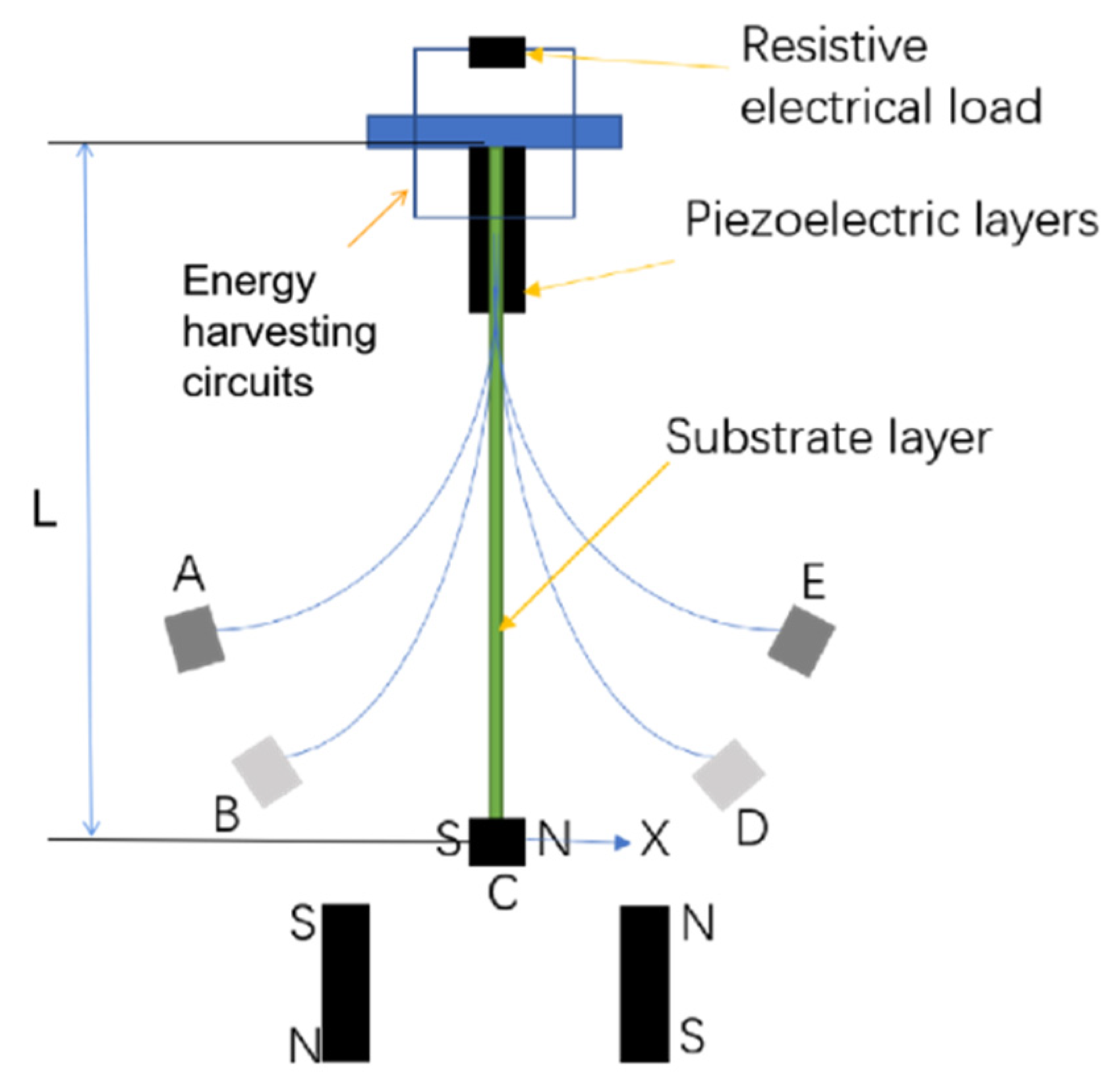
The simplified diagram of the considered tristable piezoelectric energy harvester [10] is shown in Figure 1 where X is the horizontal displacement of the end of the substrate layer at moment t, L the length of the substrate layer. In Figure 1, the magnet at the end of the substrate layer provides nonlinear forces via interacting with the other two magnets; B and D are unstable positions of the vibrating system, A, C and E are stable ones. The energy is stored by the energy harvesting circuits based on the piezoelectric effect of the piezoelectric layers driven by the substrate layer. According to the Second Law of Newton and Kirchhoff’s law, the vibrating system of the energy harvester can be expressed as
m X ¨ ( t ) + c X ˙ ( t ) + k ( X ) k e m V ( t ) = F cos ( Ω t ) , c p V ˙ ( t ) + V ( t ) r l + k e m X ˙ ( t ) = 0
where m, c, kem are the equivalent mass, the equivalent damping and equivalent electromechanical coupling coefficient, respectively; cp is the equivalent capacitance of the piezoelectric materials, r l the load resistance, V(t) the voltage across the electrical load, X(t) is the tip displacement of the harvester in the transverse direction, k(X) the magnetic force whose nonlinearity due to the effect of magnetic force, and F and Ω are the amplitude and frequency of the external excitation, respectively. The polynomial form for nonlinear magnetic force [15,17] is introduced in order to characterize the relationship between the tip displacement of the cantilever and it below:
k ( X ) = a 1 X a 2 X 3 + a 3 X 5
where a 1 , a 2 and a 3 are positive and the coefficients of the polynomial. By introducing the dimensionless time T = ω 0 t where ω 0 = a 1 m , and the variables x ( T ) = X ( t ) L , v ( T ) = V ( t ) V 0 , the dimensionless form of Equation (1) can be expressed by
x ( T ) + μ x ( T ) + x ( T ) k 1 x 3 ( T ) + k 2 x 5 ( T ) η v ( T ) = f 0 cos ω T , v ( T ) + γ v ( T ) + β x ( T ) = 0 ,
where
ω = Ω ω 0 , k 1 = a 2 a 1 L 2 , k 2 = a 3 a 1 L 4 , μ = c m ω 0 , η = k e m V 0 L a 1 , f 0 = F L a 1 , γ = 1 c p r l ω 0 , β = k e m L c p V 0 .
By denoting x ( T ) x ,   v ( T ) v ,   x ( T ) x ˙ ,   x ( T ) x ¨ ,   v ( T ) v ˙ in Equation (3), the dimensionless state-space model of the piezoelectric vibration energy harvesting system can be obtained as follows:
x ¨ + μ x ˙ + x k 1 x 3 + k 2 x 5 η v = f 0 cos ( ω T ) , v ˙ + γ v + β x ˙ = 0 .
Note that all non-dimensional parameters in the above equation are positive. The nomenclatures of the system parameters are presented in Table 1.
Assuming μ = 0, η = 0, and f0 = 0 in Equation (5) yields its unperturbed system
x ˙ = y , y ˙ = x + k 1 x 3 k 2 x 5 .
which is a Hamilton system. Letting the right side of Equation (6) be zero, one obtains its equilibria whose vertical coordinate y is zero and horizontal coordinates satisfy
x ( 1 k 1 x 2 + k 2 x 4 ) = 0 .
Their stability is determined by the roots of the following characteristic equation
λ 2 + ( 1 3 k 1 x 2 + 5 k 2 x 4 ) = 0 .
Obviously, the origin O(0, 0) is the equilibrium of the system (6) whose eigenvalue is λ = ± i , implying that O(0, 0) is a center. The number of the nontrivial equilibria and the shapes of possible potential wells of the unperturbed system (6) depend on the non-dimensional parameters k1 and k2. For example, for k 1 2 < 4 k 2 , there is no nontrivial equilibria in Equation (7), because according to Weda’s Theorem, apart from zero, there are no real roots of x 2 in Equation (7). For k 1 2 > 4 k 2 , We have the following theorem.
Theorem 1.
If  k 1 2 > 4 k 2 , there will be four nontrivial equilibria of Equation (7), i.e., two centers and two saddles.
Proof of Theorem 1.
If k 1 2 > 4 k 2 , according to Weda’s Theorem, there are two pairs of positive roots of x 2 in Equation (7) expressed by k 1 ± Δ 2 k 2 where Δ = k 1 2 4 k 2 > 0 ; thus, there are four real solutions of x in Equation (7), namely, ± k 1 + Δ 2 k 2 and ± k 1 Δ 2 k 2 .
In the neighborhood of the two equilibria S ± ( ± k 1 Δ 2 k 2 , 0 ) , the two eigenvalues solved from Equation (8) are a positive one and a negative one, expressed by λ = ± Δ ( k 1 Δ ) k 2 , respectively. It means that S ± ( ± k 1 Δ 2 k 2 , 0 ) are saddles. In the neighborhood of the other two nontrivial equilibria C ± ( ± k 1 + Δ 2 k 2 , 0 ) , the characteristic equation becomes
λ 2 + Δ ( k 1 + Δ ) k 2 = 0 .
As Δ ( k 1 + Δ ) k 2 > 0 , there are two pure imaginary roots in the above equation, illustrating that the equilibria C ± ( ± k 1 + Δ 2 k 2 , 0 ) are centers. □
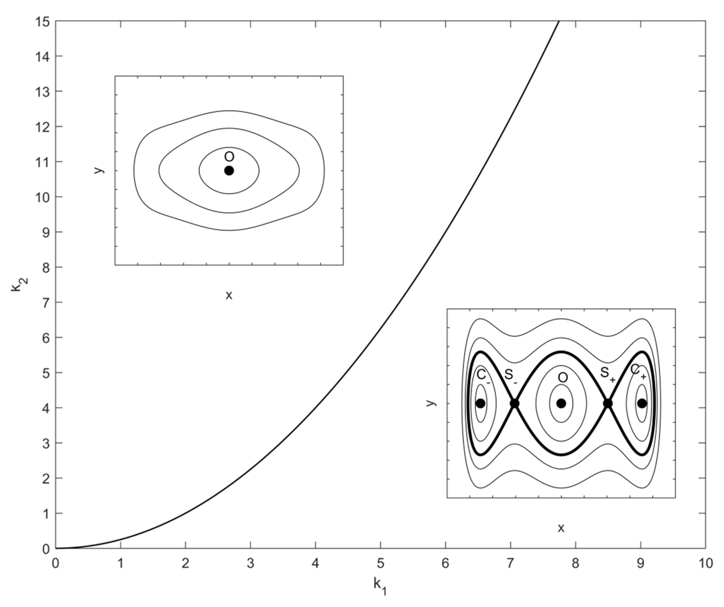
Accordingly, the critical condition for static bifurcation of the equilibria is k 1 2 = 4 k 2 . The different types of orbits of the unperturbed system (6) are classified in k1-k2 plane, as shown in Figure 2. It follows that for a given value of the dimensionless cubic stiffness term k1, the lower the dimensionless penta power stiffness term k2 is, the higher the probability of a triple well the system will have. Based on the relationship between the dimensionless parameters and the original parameters shown in Equation (4), it indicates that the lower the penta power stiffness coefficient of polynomial magnetic force a 3 is, the higher possibility for the occurrence of a triple potential well will be. For the case of multiple equilibria, two nontrivial equilibria C ± ( ± k 1 + Δ 2 k 2 , 0 ) are the centers of two potential wells surrounded by homoclinic orbits, the origin is the center of a well surrounded by heteroclinic orbits crossing the other two nontrivial saddles S ± ( ± k 1 Δ 2 k 2 , 0 ) . As well known, multiple wells may induce multistability [25,26]. In the following sections, we consider the case of three potential energy wells, and focus on how to make use of the external excitation and initial conditions to induce complex dynamics such as jump phenomena among periodic attractors, inter-well oscillation or even chaos, thus harvesting vibration energy effectively. All the values of system parameters are dimensionless for analysis. Based on the physical properties of the energy harvester in reference [10], some invariable parameters can be set as:
k 1 = 8 , k 2 = 12 , μ = 0.1 , η = 0.1 , γ = 0.1 , β = 0.1 .
The parameters f 0 and ω will be changed to study the influence mechanism of dynamical response characteristics. It can be calculated that the horizontal coordinates for the two nontrivial centers C ± ( ± x c , 0 ) and saddles S ± ( ± x s , 0 ) are x c = ± 2 2 and x s = ± 6 6 , respectively.

3. Periodic Responses

3.1. Periodic Solutions near the Origin (0, 0)

In this subsection, we consider the periodic solutions near the equilibrium (0, 0). First, by introducing a small parameter ε satisfying 0 < ε≪1 and rescaling the parameters μ , γ , η and f 0 in Equation (5) as
μ = ε μ ˜ , γ = ε γ ˜ , η = ε η ˜ , f 0 = ε 2 f ˜ ,
one can rewrite the system (5) as
x ¨ + x = ε μ ˜ x ˙ + ε 2 f ˜ cos ω T + ε η ˜ v + k 1 x 3 k 2 x 5 , v ˙ + ε γ ˜ v = β x ˙ .
The Method of Multiple Scales (MMS) [15] is employed to obtain the approximate-analytical solution of Equation (12). To this end, the displacement x and voltage response v are expanded as
x = ε x 1 + ε 2 x 2 + ε 3 x 3 + ,   v = ε v 1 + ε 2 v 2 + ε 3 v 3 + .
The time derivatives can be rewritten as
T i = ε i T , D i = T i , d d T = i = 0 n ε i D i ( i = 0 , 1 , ) .
Considering harmonic resonance, it is assumed that
ω = 1 + ε σ
where the detuning parameter σ = O ( 1 ) . Introducing Equations (13)–(15) into Equation (12) and separating the coefficients of ε1, ε2 and ε3 leads to
ε 1 : D 0 2 x 1 + ω 2 x 1 = 0 , D 0 v 1 = β D 0 x 1 ,
ε 2 : D 0 2 x 2 + ω 2 x 2 = 2 D 0 D 1 x 1 μ ˜ D 0 x 1 + f ˜ cos ω T 0 + η ˜ v 1 + 2 σ ω x 1 , D 0 v 2 = γ ˜ v 1 β ( D 1 x 1 + D 0 x 2 ) D 1 v 1 ,
and
ε 3 : D 0 2 x 3 + ω 2 x 3 = D 1 2 x 1 2 D 2 D 0 x 1 2 D 1 D 0 x 2 μ ˜ ( D 1 x 1 + D 0 x 2 ) + η ˜ v 2 + 2 σ ω x 2 x 1 σ 2 + k 1 x 1 3 .
The solution of Equation (16) can be assumed as
x 1 = A ( T 1 , T 2 ) e i ω T 0 + c c , v 1 = β A e i ω T 0 + c c
where cc represents the complex conjugate of the preceding terms, and the complex slow-times dependent amplitude A ( T 1 , T 2 ) is expressed as A = a ( T 1 , T 2 ) 2 e i θ . Here, the a ( T 1 , T 2 ) and θ are real, representing the real amplitude and the phase difference of the periodic solution x 1 , respectively. By substituting the solution (19) into Equation (17) and separating the secular terms, one has
D 1 A = μ ˜ A 2 i f ˜ 4 ω + η ˜ β A i 2 ω i σ A .
Since A is the function of T 1 and T 2 , it can be solved from Equation (17) that
x 2 = 0 ,   v 2 = β γ ˜ A i ω + c c .
Submitting Equations (19) and (21) into Equation (13), one can approximately express the periodic solution x as x = ε a cos ( ω T 0 + θ ) . Substituting Equations (19)–(21) into Equation (18) and separating its secular terms yields
D 2 A = f ˜ β η ˜ i 16 ω 3 A β 2 η ˜ 2 i 8 ω 3 A β η ˜ γ ˜ 2 ω 2 + f ˜ μ ˜ 16 ω 2 f ˜ σ i 8 ω 2 + A β η ˜ σ i 2 ω 2 3 k 1 A 2 A ¯ 2 ω A μ ˜ 2 i 8 ω .
Letting the amplitude of x be a ^ = ε a , considering A ˙ D 0 A + ε D 1 A + ε 2 D 2 A , substituting Equations (20) and (22) into it and returning its parameters to the original dimensionless parameters of Equation (5), one obtains
a ^ ˙ = μ 2 a ^ η β γ a ^ 2 ω 2 + f 0 μ cos θ 8 ω 2 + ( β η 6 ω 2 + 2 ω ) f 0 sin θ 8 ω 3 , a ^ θ ˙ = ( ω 1 ) a ^ η 2 β 2 a ^ 8 ω 3 + η β ( ω 1 ) a ^ 2 ω 2 3 k 1 a ^ 3 8 ω + η β a ^ 2 ω μ 2 a ^ 8 ω f 0 μ sin θ 8 ω 2 + ( β η 6 ω 2 + 2 ω ) f 0 cos θ 8 ω 3
Letting the right side of Equation (23) be zero leads to
μ 2 a ^ + η β γ a ^ 2 ω 2 = f 0 μ cos θ 8 ω 2 + ( β η 6 ω 2 + 2 ω ) f 0 sin θ 8 ω 3 , ( ω 1 ) a ^ + η 2 β 2 a ^ 8 ω 3 η β ( ω 1 ) a ^ 2 ω 2 + 3 k 1 a ^ 3 8 ω η β a ^ 2 ω + μ 2 a ^ 8 ω = f 0 μ sin θ 8 ω 2 + ( β η 6 ω 2 + 2 ω ) f 0 cos θ 8 ω 3 .
Eliminating the triangulation function of Equation (24), one can get
f 0 2 μ 2 64 ω 4 + ( β η 6 ω 2 + 2 ω ) 2 f 0 2 64 ω 6 = ( μ 2 + η β γ 2 ω 2 ) 2 a ^ 2 + ( ω 1 + η 2 β 2 8 ω 3 η β ( ω 1 ) 2 ω 2 + 3 k 1 a ^ 2 8 ω η β 2 ω + μ 2 8 ω ) 2 a ^ 2 .
To determine the stability of the periodic solution, one can get its characteristic equation. Based on Equations (23)–(25), the characteristic equation can be written as
λ 2 + ( μ + η β γ ω 2 ) λ + f 0 2 μ 2 64 ω 4 + ( β η 6 ω 2 + 2 ω ) 2 f 0 2 64 ω 6 + ( ( ω 1 ) a ^ + η 2 β 2 a ^ 8 ω 3 η β ( ω 1 ) a ^ 2 ω 2 + 3 k 1 a ^ 3 8 ω η β a ^ 2 ω + μ 2 a ^ 8 ω ) 3 k 1 a ^ 4 ω = 0
According to the equation above, the stability of the periodic solution in the neighborhood of the origin will be changed when λ = 0, namely
f 0 2 μ 2 64 ω 4 + ( β η 6 ω 2 + 2 ω ) 2 f 0 2 64 ω 6 + ( ( ω 1 ) a ^ + η 2 β 2 a ^ 8 ω 3 η β ( ω 1 ) a ^ 2 ω 2 + 3 k 1 a ^ 3 8 ω η β a ^ 2 ω + μ 2 a ^ 8 ω ) 3 k 1 a ^ 4 ω = 0 .
The frequency response curves in the neighborhood of the origin are plotted in Figure 3. In Figure 3, the branches of analytical amplitude a ^ for f0 = 0.002, 0.01 and 0.05 are obtained from Equation (25). The solid curves and the dashing ones represent the stable and unstable periodic solutions, respectively. Their stability is determined by the positive-negative sign of the real parts of eigenvalues solved from Equation (26). Based on Equation (27), one gets the saddle-node point separating the solid curve and dashing curve. The numerical results for the amplitudes of periodic responses are presented by applying the 4th Runge-Kutta approach to simulate the numerical solutions of the dimensionless system (5) via MATLAB. Definitely, the numerical approach will only produce stable solutions. As illustrated in Figure 3, there is a good agreement between the theoretical and numerical response results, implying the approximate-analytical solutions are valid. Furthermore, it follows from Figure 3 that for f0 = 0.05 and ω in the range (0.50, 0.76), the frequency response curves bend to the left and yield multivalued solutions. It means that the saddle-node bifurcation of the periodic solution around the origin O(0, 0), hence the coexistence of two intra-well attractors, can be triggered by the increase of f0 and the variation of ω in a low-frequency range.
When two intra-well attractors around the well center O(0, 0) or C ± ( ± x c , 0 ) is induced in the vicinity of the saddle-node bifurcation point, the initial conditions will determine the branch to which the response attracts. For the purpose of energy harvesting, the initial conditions should be chosen to follow the high-amplitude one in order to output high voltage consequently. That is why we present the sequences of the attractors and their basins of attraction for the variation of the dimensionless external excitation. Basin of attraction means the union of initial conditions leading to the same attractor [20,21]. If the boundary of the basin of attraction of one attractor is fractal and intermingled with another, a jump among multiple attractors may easily occur. In this study, the 4th Runge–Kutta approach and the point-mapping method [26] are employed to describe the basin of attraction. The basins of attraction are drawn in the initial-condition plane −1.0 ≤ x(0) ≤ 1.0, −1.0 ≤ y(0) ≤ 1.0 by generating a 600 × 600 array of starting conditions, for each of the initial points. The time step is taken as 0.01. For each figure of sequences of attractors and their basins of attraction, there are pairs of pictures on each line of which the left one is the phase map of the attractors, while the right one shows their basins of attraction. For each attractor, its basin of attraction is marked in the same color as its phase map.
Given f 0 = 0.05 , the sequences of attractors and their basins of attraction with the variation of the dimensionless excitation frequency ω are depicted in Figure 4. For ω = 0.3 (see Figure 4(a1)), there coexist three intra-well attractors around three different well centers O(0, 0) and C ± ( ± x c , 0 ) , respectively. Even though their basins of attraction in some areas entangle each other (see Figure 4(a2)), the vicinity of three potential-well centers is single-colored with clear basin boundaries, meaning that near the potential-well centers, the phenomenon jump will not occur. Only if the initial condition of the structure changes dramatically from the neighborhood of one center to another, there will be a jump between two intra-well attractors. It is worth mentioning that the attractors are around different potential-well centers, thus jump is an inter-well jump. The amplitudes of the three attractors are very low, contributing little to harvest energy. Comparatively, the inter-well jump caused by the change of initial conditions contributes more to energy harvesting. As ω increases to 0.55, there are four intra-well attractors coexisting (see Figure 4(b1)). Apart from the three intra-well attractors, a new intra-well attractor around O(0, 0) with a much higher amplitude appears. However, as can be observed in Figure 4(b2), its basin of attraction is fractal and hard to be detected. Hence, it is a so-called rare attractor [27] whose occurring probability is very low. Compared with the basin map in Figure 4(a2), a better point is that outside of the vicinity of the three well centers, the fractality extent of the basins of attraction becomes more severe, meaning that jump can be triggered more easily in this region. When ω grows to 0.75, the occurrence probability of the higher-amplitude intra-well attractor around O(0, 0) is much higher, because its basin of attraction grows larger, especially in the neighborhood of O(0, 0) (see Figure 4(c2)). Note that the phenomenon of jump between the two intra-well attractors around O(0, 0), namely the intra-well jump, more easily occurs than the inter-well jump, which will be beneficial for energy harvesting. As ω increases to 1.0, the lower-amplitude intra-well attractor around O(0, 0) disappears; still there coexist three attractors, as shown in Figure 4(d1). Based on their basins of attraction in Figure 4(d2), it is obvious that a better energy harvesting performance can be given by the higher-amplitude intra-well oscillation around O(0, 0) or the inter-well jump led by the dramatic change of initial conditions.

3.2. Periodic Solutions near the Nontrivial Equilibria ( ± x c , 0)

Around the nontrivial equilibria ( ± x c , 0), the periodic vibration of the cantilever beam structure can be induced by the perturbation of the two nontrivial centers of the unperturbed system (6) (see C and C+ in Figure 2). To begin with, supposing x = ± x c + x ^ , and rescaling the system parameters by Equation (11) yields
x ^ ¨ + ω ^ 2 x ^ = ε μ ˜ x ^ ˙ + ε 2 f ˜ cos ω T + ε η ˜ v Q 1 x ^ 2 Q 2 x ^ 3 k 2 ( ± 5 x c x ^ 4 + x ^ 5 ) , v ˙ + ε γ ˜ v = β x ^ ˙ .
where
ω ^ 2 = 1 3 k 1 x c 2 + 5 k 2 x c 4 ,   Q 1 = 10 k 2 x c 3 3 k 1 x c ,   Q 2 = 10 k 2 x c 2 k 1 .
It can be calculated that ω ^ = 2 , Q 1 = 25.46 and Q 2 = 52 , all positive. To apply the Method of Multiple Scales, assuming harmonic resonance in the system (28) that
ω = ω ^ + ε σ ^ ,
where σ ^ is the detuning parameter, rescaling x ^ and voltage response v in Equation (28) as
x ^ = ε x ^ 1 + ε 2 x ^ 2 + + ε 3 x ^ 3 , v = ε v ^ 1 + ε 2 v ^ 2 + ε 3 v ^ 3 ,
and comparing the coefficients of ε1, ε2 and ε3 in the system (28), respectively, one has
ε 1 : D 0 2 x ^ 1 + ω 2 x ^ 1 = 0 , D 0 v ^ 1 = β D 0 x ^ 1 ,
ε 2 : D 0 2 x ^ 2 + ω 2 x ^ 2 = 2 D 0 D 1 x ^ 1 μ ˜ D 0 x ^ 1 + f ˜ cos ω T 0 + η ˜ v ^ 1 + 2 σ ω x ^ 1 Q 1 x ^ 1 2 , D 0 v ^ 2 = γ ˜ v ^ 1 β ( D 1 x ^ 1 + D 0 x ^ 2 ) D 1 v ^ 1 ,
and
ε 3 : D 0 2 x ^ 3 + ω 2 x ^ 3 = D 1 2 x ^ 1 2 D 2 D 0 x ^ 1 2 D 1 D 0 x ^ 2 μ ˜ ( D 1 x ^ 1 + D 0 x ^ 2 ) + η ˜ v ^ 2 + 2 σ ω x ^ 2 x ^ 1 σ 2 2 Q 1 x ^ 1 x ^ 2 Q 2 x ^ 1 3 .
The solution of Equation (32) can be written as
x ^ 1 = B ( T 1 , T 2 ) e i ω T 0 + c c , v ^ 1 = β B e i ω T 0 + c c ,
where the complex slow-times dependent amplitude B ( T 1 , T 2 ) is given by
B = b ( T 1 , T 2 ) 2 e i φ ( T 1 , T 2 ) .
In Equation (36), b ( T 1 , T 2 ) and φ ( T 1 , T 2 ) are real, representing the real amplitude and the phase difference of the periodic solution x ^ 1 , respectively. Substituting Equation (35) into Equation (33) and separating its secular terms leads to
D 1 B = μ ˜ B 2 i f ˜ 4 ω + η ˜ β B i 2 ω i σ B ,
and
x ^ 2 = ± ( 2 Q 1 B B ¯ ω 2 + Q 1 B 2 3 ω 2 e 2 i ω T 0 + Q 1 B ¯ 2 3 ω 2 e 2 i ω T 0 ) , v ^ 2 = β Q 1 B 2 3 ω 2 e 2 i ω T 0 γ ˜ β B i ω e i ω T 0 + c c ,
substituting Equations (35), (37) and (38) into Equation (34) and separating the secular terms there yields
D 2 B = f ˜ β η ˜ i 16 ω 3 B β 2 η ˜ 2 i 8 ω 3 B β η ˜ γ ˜ 2 ω 2 + f ˜ μ ˜ 16 ω 2 f ˜ σ i 8 ω 2 + B β η ˜ σ i 2 ω 2 + 3 Q 2 B 2 B ¯ i 2 ω 5 Q 1 2 B 2 B ¯ i 3 ω 3 B μ ˜ 2 i 8 ω .
Considering B ˙ D 0 B + ε D 1 B + ε 2 D 2 B and b ^ = ε b , substituting Equations (36), (37) and (39) into it and expressing it by the original dimensionless parameters of Equation (5), one has:
b ^ ˙ = μ 2 b ^ η β γ b ^ 2 ω 2 + f 0 μ cos φ 8 ω 2 + ( β η 6 ω 2 + 2 ω ω ^ ) f 0 sin φ 8 ω 3 , b ^ φ ˙ = ( ω ω ^ ) b ^ η 2 β 2 b ^ 8 ω 3 + η β ( ω ω ^ ) b ^ 2 ω 2 + 3 Q 2 b ^ 3 8 ω 5 Q 1 2 b ^ 3 12 ω 3 + η β b ^ 2 ω μ 2 b ^ 8 ω f 0 μ sin φ 8 ω 2 + ( β η 6 ω 2 + 2 ω ω ^ ) f 0 cos φ 8 ω 3
For the periodic solution around C or C+, the right side of Equation (40) is zero, i.e.,
μ 2 b ^ + η β γ b ^ 2 ω 2 = f 0 μ cos θ 8 ω 2 + ( β η 6 ω 2 + 2 ω ω ^ ) f 0 sin θ 8 ω 3 , ( ω ω ^ ) b ^ + η 2 β 2 b ^ 8 ω 3 η β ( ω ω ^ ) b ^ 2 ω 2 3 Q 2 b ^ 3 8 ω + 5 Q 1 2 b ^ 3 12 ω 3 η β b ^ 2 ω + μ 2 b ^ 8 ω = f 0 μ sin θ 8 ω 2 + ( β η 6 ω 2 + 2 ω ω ^ ) f 0 cos θ 8 ω 3 .
Eliminating the triangulation function of Equation (41), one obtains
f 0 2 μ 2 64 ω 4 + ( β η 6 ω 2 + 2 ω ω ^ ) 2 f 0 2 64 ω 6 = ( μ 2 + η β γ 2 ω 2 ) 2 b ^ 2 + ( ω ω ^ + η 2 β 2 8 ω 3 η β ( ω ω ^ ) 2 ω 2 3 Q 2 b ^ 2 8 ω + 5 Q 1 2 b ^ 2 12 ω 3 η β 2 ω + μ 2 8 ω ) 2 b ^ 2 .
The periodic solution near the nontrivial equilibria ( ± x c , 0) can be expressed as
x = ± x c 2 Q 1 b ^ 2 3 ω 2 + b ^ cos ( ω T + φ ) ± Q 1 b ^ 2 3 ω 2 cos 2 ( ω T + φ ) ) .
As in Section 3.1, the stability of the periodic solutions can be determined by the following characteristic equation
λ 2 + ( μ + η β γ ω 2 ) λ + f 0 2 μ 2 64 ω 4 + ( β η 6 ω 2 + 2 ω ω ^ ) 2 f 0 2 64 ω 6 + ( ( ω ω ^ ) b ^ + η 2 β 2 b ^ 8 ω 3 η β ( ω ω ^ ) b ^ 2 ω 2 3 Q 2 b ^ 3 8 ω + 5 Q 1 2 b ^ 3 12 ω 3 η β b ^ 2 ω + μ 2 b ^ 8 ω ) ( 5 Q 1 2 b ^ 6 ω 3 3 Q 2 b ^ 4 ω ) = 0 .
Hence, saddle-node bifurcation will occur when
f 0 2 μ 2 64 ω 4 + ( β η 6 ω 2 + 2 ω ω ^ ) 2 f 0 2 64 ω 6 + ( ( ω ω ^ ) b ^ + η 2 β 2 b ^ 8 ω 3 η β ( ω ω ^ ) b ^ 2 ω 2 3 Q 2 b ^ 3 8 ω + 5 Q 1 2 b ^ 3 12 ω 3 η β b ^ 2 ω + μ 2 b ^ 8 ω ) ( 5 Q 1 2 b ^ 6 ω 3 3 Q 2 b ^ 4 ω ) = 0
According to Equations (42)–(45), the frequency response curves in the neighborhood of the nontrivial equilibria are presented in Figure 5 where the branches of analytical amplitude b ^ for f0 = 0.002, 0.01 and 0.05 are obtained from Equation (42). The solid curves and the dashed ones show the stable and unstable periodic solutions, respectively. Their stability is determined by the positive-negative sign of the real parts of eigenvalues solved from Equation (44). The saddle-node point separating the solid curve and dashing curve is determined by Equation (45). By applying 4th Runge–Kutta approach to simulate the numerical solutions of the dimensionless system (5), the numerical results are presented. As shown in Figure 5, theoretical results totally agree with the numerical ones. Similar to Figure 3, it also can be observed in Figure 5 that for f0 = 0.05, the frequency response curves bend to the left and yield bistability, indicating that due to saddle-node bifurcation of the periodic solution, in the vicinity of the saddle-node bifurcation point, there are two intra-well periodic attractors around each nontrivial equilibrium.
Based on the analysis of the periodic responses near the origin and the nontrivial equilibria, the evolution of the periodic solutions of system (5) with the amplitude of f0 for ω = 1.5 is illustrated in Figure 6. Obviously, when f0 increases from 0, the nontrivial equilibria and the origin lose their stability; instead, three periodic attractors coexist, attributed to the disturbance of the tristable equilibria. When f0 varies from 0 to 0.02, the numerical simulation is in great agreement with the theoretical solution. However, when f0 continues to increase, the theoretical prediction of the periodic responses does not match the numerical results well, which may be due to the limitation of the Method of Multiple Scale, namely the value of the excitation frequency ω should be closed to the inherent frequency of the perturbed systems (12) and (28) near the origin and the nontrivial equilibria ( ± x c , 0). Actually, the given value of the excitation frequency is ω = 1.5, while the inherent frequencies of the systems (12) and (28) are 1 and 2, respectively. It means that the derivations of ω from the two inherent frequencies are not that small. Although the prediction is not that quantitatively accurate, the theoretical results and numerical simulation both show that the increase of the excitation amplitude triggers bistability around each nontrivial well center ( ± x c , 0). According to the theoretical analysis, it can be ascribed to the saddle-node bifurcation of the periodic solutions. For instance, for f0 = 0.05, there coexist five intra-well periodic attractors, i.e., two around each nontrivial potential-well center and one around O(0, 0).
Fixing ω = 1.5, the evolution of periodic responses and their basins of attraction with the increase of the dimensionless excitation amplitude f0 is shown in Figure 7. For f0 = 0, the coexisting triple attractors are the three well centers whose basin boundaries are smooth, as shown in Figure 7(a1,a2). For f0 = 0.045, the three point attractors are perturbed and replaced by three intra-well periodic attractors around them (see Figure 7(b1)). Although the single-colored neighborhood of each well center in Figure 7(b2) implies that the initial conditions chosen there must attract to the intra-well attractor around it, the inter-well jump may be triggered when the initial conditions are disturbed dramatically. As f0 increases a bit to reach 0.046, two new intra-well periodic attractors with higher amplitudes suddenly appear in the neighborhood of the nontrivial well centers. As predicted in Figure 6, this can be attributed to the saddle-node bifurcation. Now, there are five intra-well attractors in Figure 7(c1). However, as shown in Figure 4(c2), the basins of attraction of the new attractors are fractal and scattered. Thus, the occurring probability for these two high-amplitude intra-well responses is very low. As f0 continues to increase, the basins of attraction of the two new periodic attractors are enlarged (see Figure 7(d2)). It means that the occurrence probability of the higher-amplitude intra-well attractors around the well centers C and C+ is much higher. Moreover, the jump between the two intra-well attractors around each nontrivial well center, namely the intra-well jump, is of higher probability to occur. Therefore, not only the intra-well jump due to saddle-node bifurcation of the periodic solution around the nontrivial well centers and a small perturbation of the initial condition but also the inter-well jump among attractors around different wells that is led by dramatic disturbance of the initial condition can make the structure harvest vibration energy more conveniently.

4. Global Bifurcation

In this section, we discuss the necessary conditions for heteroclinic and homoclinic bifurcation and the complex dynamics that these global bifurcations induce. To begin with, the heteroclinic orbits and homoclinic orbits are written as [20]:
x h e t e r o = ± 2 x s sinh ( χ T 2 ) ( κ + cosh ( χ T ) ) 1 2 , y h e t e r o = ± 2 x s χ ( 1 + κ ) cosh ( χ T 2 ) 2 ( κ + cosh ( χ T ) ) 3 2 .
and
x homo = ± 2 x s cosh ( χ T 2 ) ( κ + cosh ( χ T ) ) 1 2 , y homo = 2 x s χ ( κ + 1 ) sinh ( χ T 2 ) 2 ( κ + cosh ( χ T ) ) 3 2 .
where
χ = x s 2 2 k 2 ( x c 2 x s 2 1 ) , κ = 3 x c 2 5 x s 2 3 x c 2 x s 2 > 0 .
The expression of the component v h e t e r o and v homo of the heteroclinic orbits and homoclinic ones obtained by solving Equation (5) is presented as follows
v h e t e r o ( T ) = β e γ T 0 T e γ T ˜ y h e t e r o ( T ˜ ) d T ˜ , v homo ( T ) = β e γ T 0 T e γ T ˜ y homo ( T ˜ ) d T ˜ .
The dimensionless Equation (5) is approximated to
x ˙ = y , y ˙ = x + k 1 x 3 k 2 x 5 + ε ( μ ˜ y + f ^ cos ω T + η ˜ v ) , v ˙ = γ v β y .
Since the system (50) is a time-periodic perturbation of a Hamiltonian system, the Melnikov method can be used to describe how the heteroclinic/homoclinic orbits break up in the presence of the perturbation [28]. According to the Melnikov method, the Melnikov function is a signed measure of the distance between the stable and unstable manifolds for the perturbed system [29,30]. If it has simple zeros, there will be intersection of heteroclinic orbits or homoclinic orbits, corresponding to heteroclinic bifurcation or homoclinic bifurcation, respectively. Submitting Equations (46)–(49) to its Melnikov functions under the two types of orbits yield
M h e t e r o ± ( T 0 ) = ε + y h e t e r o ( T ) ( μ ˜ y h e t e r o ( T ) + f ^ cos ( ω ( T T 0 ) ) + η ˜ v h e t e r o ( T ) ) d T = μ x s 2 χ 4 ( 1 κ ) 1 κ 2 I 1 h e t e r o η β x s 2 χ 2 ( 1 + κ ) 2 2 I 2 h e t e r o + 2 π ω χ f 0 x s csch π ω χ cos ( ω T 0 )
and
M homo ± ( T 0 ) = ε + y homo ( T ) ( μ ˜ y homo ( T ) + f ^ cos ( ω ( T T 0 ) ) + η ˜ v homo ( T ) ) d T = μ x s 2 χ 4 ( 1 κ ) 1 κ 2 I 1 homo η β x s 2 χ 2 ( 1 + κ ) 2 2 I 2 homo 2 f 0 x s sin ( 2 ω χ ) sin ( ω T 0 )
where
I 1 h e t e r o = 2 κ 1 κ 2 + 2 4 κ arctan 1 κ 1 κ 2 ,     I 2 h e t e r o = cos h ( χ T 2 ) e γ T κ + cos h ( χ T ) 3 2 ( 0 T e γ T ˜ cos h ( χ T ˜ 2 ) κ + cos h ( χ T ˜ ) 3 2 d T ˜ ) d T , I 1 homo = 2 κ 1 κ 2 2 4 κ arctan κ + 1 1 κ 2 ,   I 2 homo = sin h ( χ T 2 ) e γ T κ + cos h ( χ T ) 3 2 ( 0 T e γ T ˜ sin h ( χ T ˜ 2 ) κ + cos h ( χ T ˜ ) 3 2 d T ˜ ) d T .
In the above equation, the integrals I 2 h e t e r o and I 2 homo can be evaluated numerically [20]; I 1 h e t e r o , I 1 homo , I 2 h e t e r o and I 2 homo are all positive.
For
f 0 > f 0 h e t e r o = μ x s χ 2 sinh ( π ω χ ) 8 π ω ( 1 κ ) 1 κ 2 I 1 h e t e r o + η β x s χ 3 ( 1 + κ ) 2 sinh ( π ω χ ) 4 π ω I 2 h e t e r o ,
there will be a real number of T 0 satisfying M h e t e r o ± ( T 0 ) = 0 and M h e t e r o ± ( T 0 ) 0 , meaning that the equilibria of Equation M h e t e r o ± ( T 0 ) = 0 are simple, enabling the existence of the transverse heteroclinic orbits. Accordingly, f 0 h e t e r o is the amplitude threshold of heteroclinic bifurcation. Similarly, it follows from the Melnikov function (52) that if
f 0 > f 0 homo = μ x s χ 8 ( 1 κ ) 1 κ 2 csc ( 2 ω χ ) I 1 homo + η β x s χ 2 ( 1 + κ ) 2 4 csc ( 2 ω χ ) I 2 homo ,
the equation M h o m o ± ( T 0 ) = 0 will have simple equilibria, corresponding to an intersection of the stable and unstable manifolds and the occurrence of homoclinic bifurcation. Given ω = 1.5, critical values can be calculated that f 0 homo 0.089 and f 0 h e t e r o 0.27 .
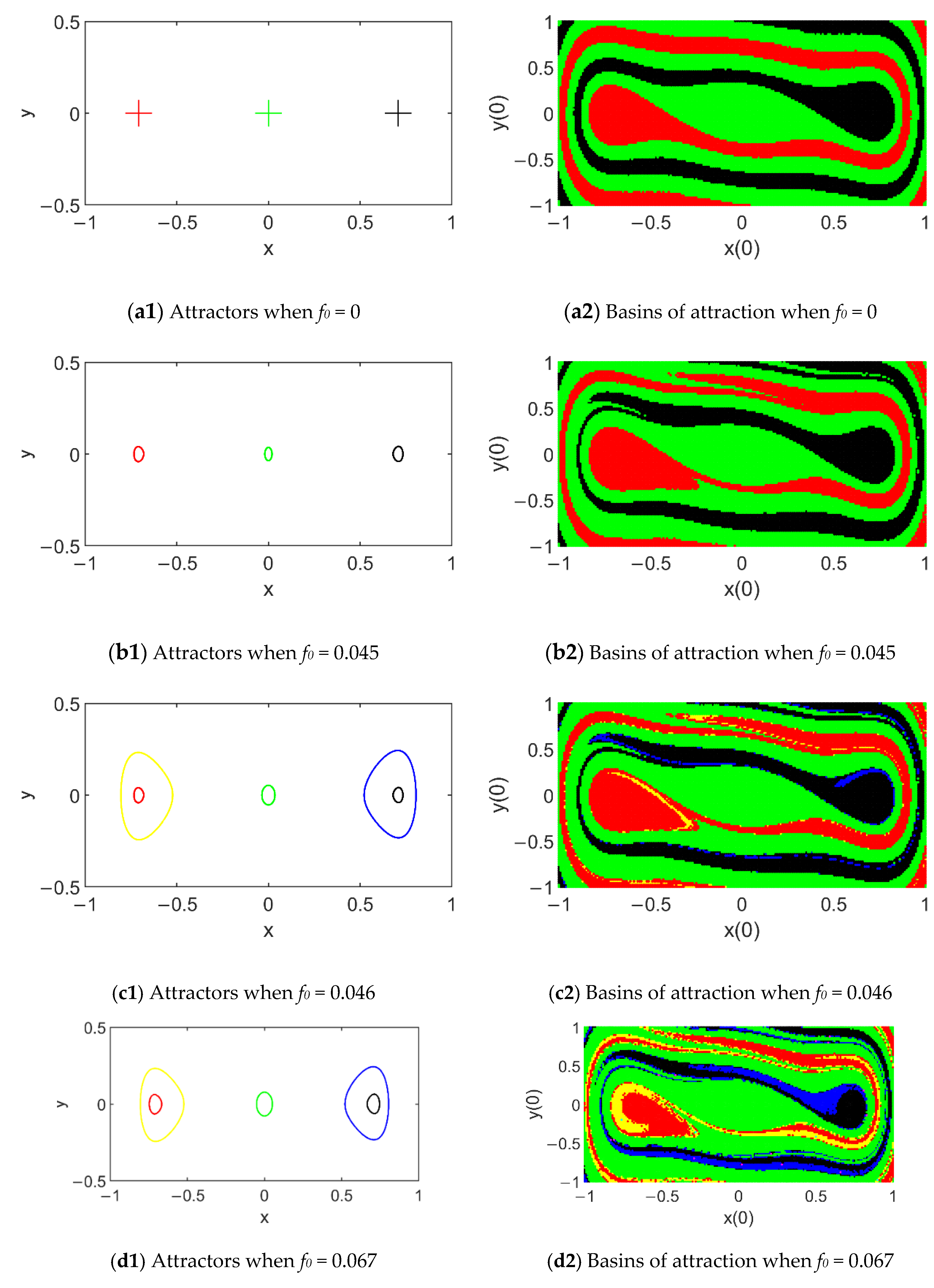
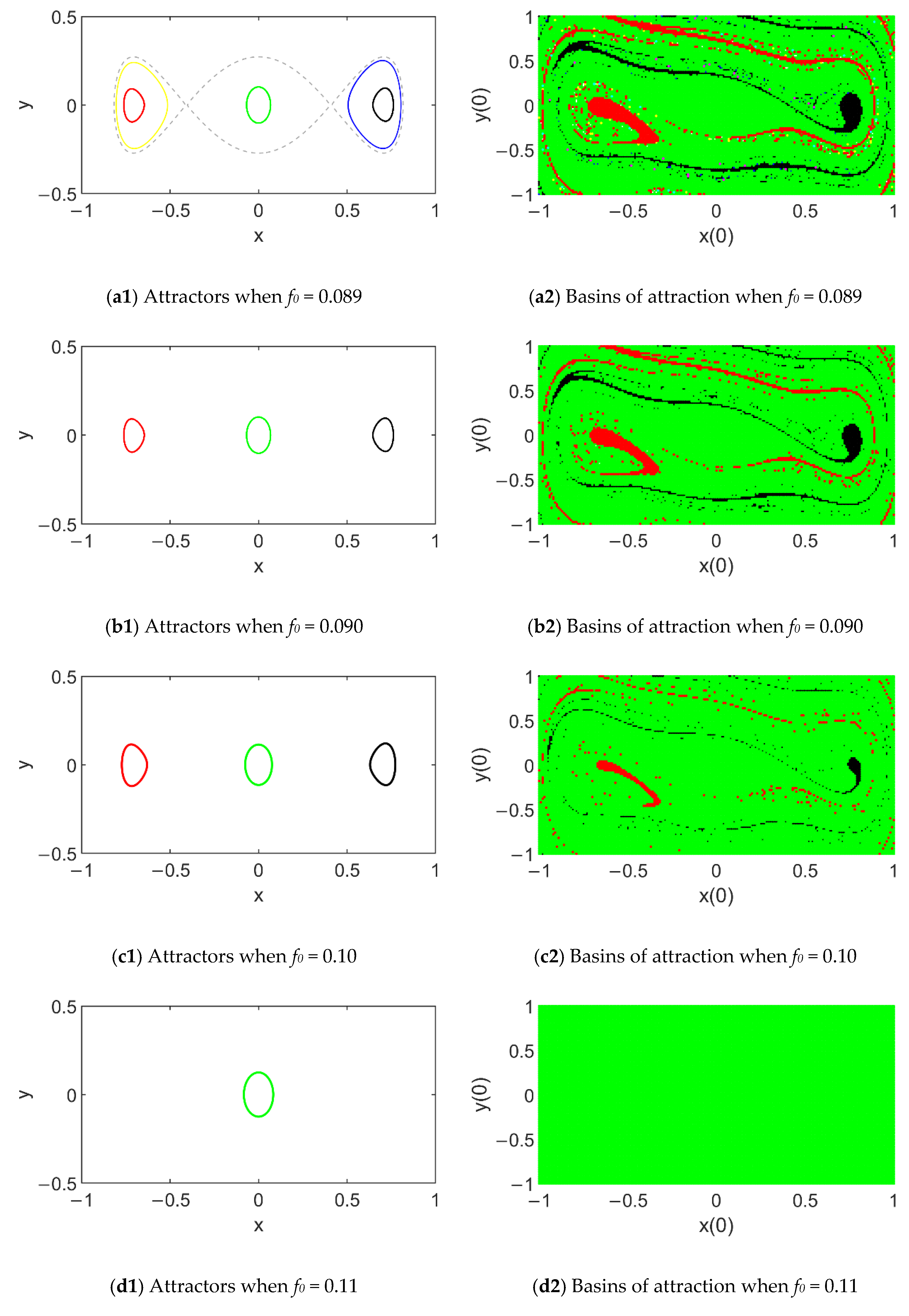
A question is then aroused: what dynamical behaviors will be induced by the global bifurcations? To get the answer, we continue to depict the evolution of attractors and their basins of attraction with the excitation amplitude f 0 for ω = 1.5 (see Figure 8). For f 0 = 0.089 (see Figure 8(a1)), the same as the case of f 0 = 0.067 (see Figure 7(d1)), there are still five periodic attractors. To be different, the two higher-amplitude intra-well attractors, i.e., the periodic attractors in yellow and blue, are expanded so that their phases nearly touch the homoclinic obits (see the light grey dashing curves in Figure 8(a1)); meanwhile, it is hard to observe their basins of attraction in Figure 8(a2), as they are eroded seriously. It indicates that for f 0 = 0.089, i.e., the theoretical threshold for homoclinic bifurcation, the two higher-amplitude intra-well attractors around two nontrivial well centers become rare attractors. When f 0 increase a bit to 0.090, it can be observed in Figure 8(b1) that these two attractors disappear; three lower-amplitude intra-well attractors are left; the intra-well attractor around the origin becomes dominant, as the most area is its basin of attraction (see the green region in Figure 8(b2)). It follows from the comparison of Figure 8(a1,b1) that the homoclinic bifurcation leads to the disappearance of two higher-amplitude intra-well attractors around nontrivial well centers.
When f 0 continues to increase, the intra-well attractor around O(0, 0) will be enlarged, and its basin of attraction will erode the basins of attraction of the other two attractors seriously (see Figure 8(c2)). For f 0 = 0.11, two intra-well attractors around the nontrivial equilibria disappear (see Figure 8(d1)), and the whole initial-condition plane of 
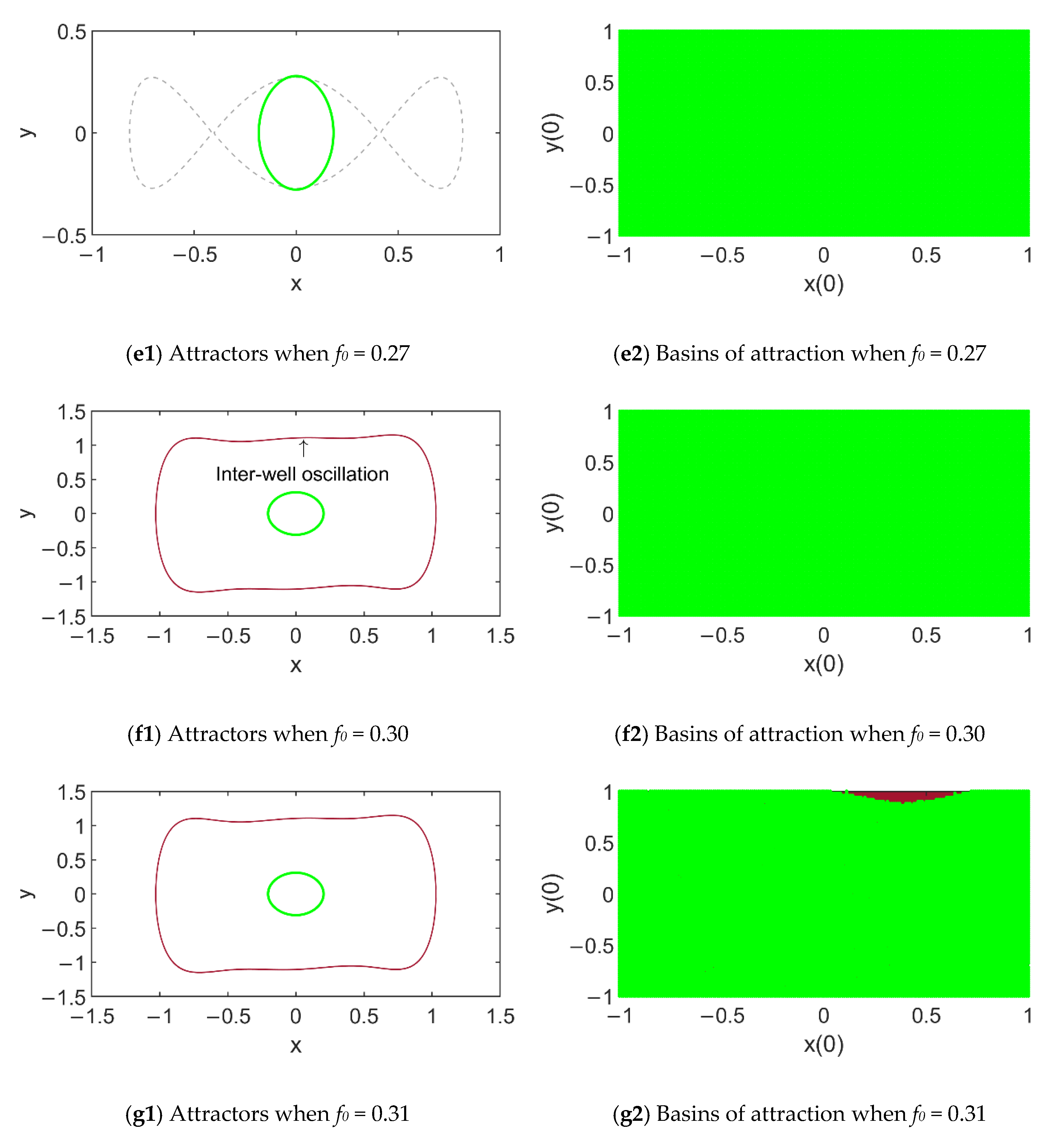
Figure 8(d2) is green, showing the global stability of the intra-well attractor around O(0, 0). There is no jump now, unfavorable for energy harvesting. As f 0 continues to increase, the situation still maintains. For f 0 = 0.27, i.e., the theoretical threshold for heteroclinic bifurcation, the phase orbit of the only attractor is enlarged and nearly touches the heteroclinic obits (see the light grey dashing curves in Figure 8(e1)); still the intra-well attractor is globally attractive, as shown in the green map in Figure 8(e2). Then, for f 0 increasing a bit to 0.30, a new periodic attractor suddenly appears (see Figure 8(f1)). It is an inter-well periodic attractor whose amplitude is much higher than the intra-well one. It can be concluded that the heteroclinic bifurcation triggers the occurrence of inter-well response. Due to the large amplitude of the inter-well attractor in Figure 8(f1), we have to expand the phase map plane to display it. Note that we still keep the initial plane −1.0 ≤ x(0) ≤ 1.0, −1.0 ≤ y(0) ≤ 1.0 which is totally green, meaning that initial conditions in this region cannot lead to this attractor (see Figure 8(f2)). As f 0 grows to 0.31, one can observe its basin of attraction in the initial plane (see Figure 8(g2)). Of course, the occurrence of inter-well oscillation is advantageous for energy harvesting.
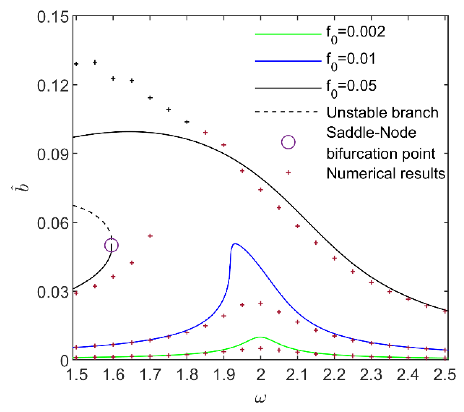
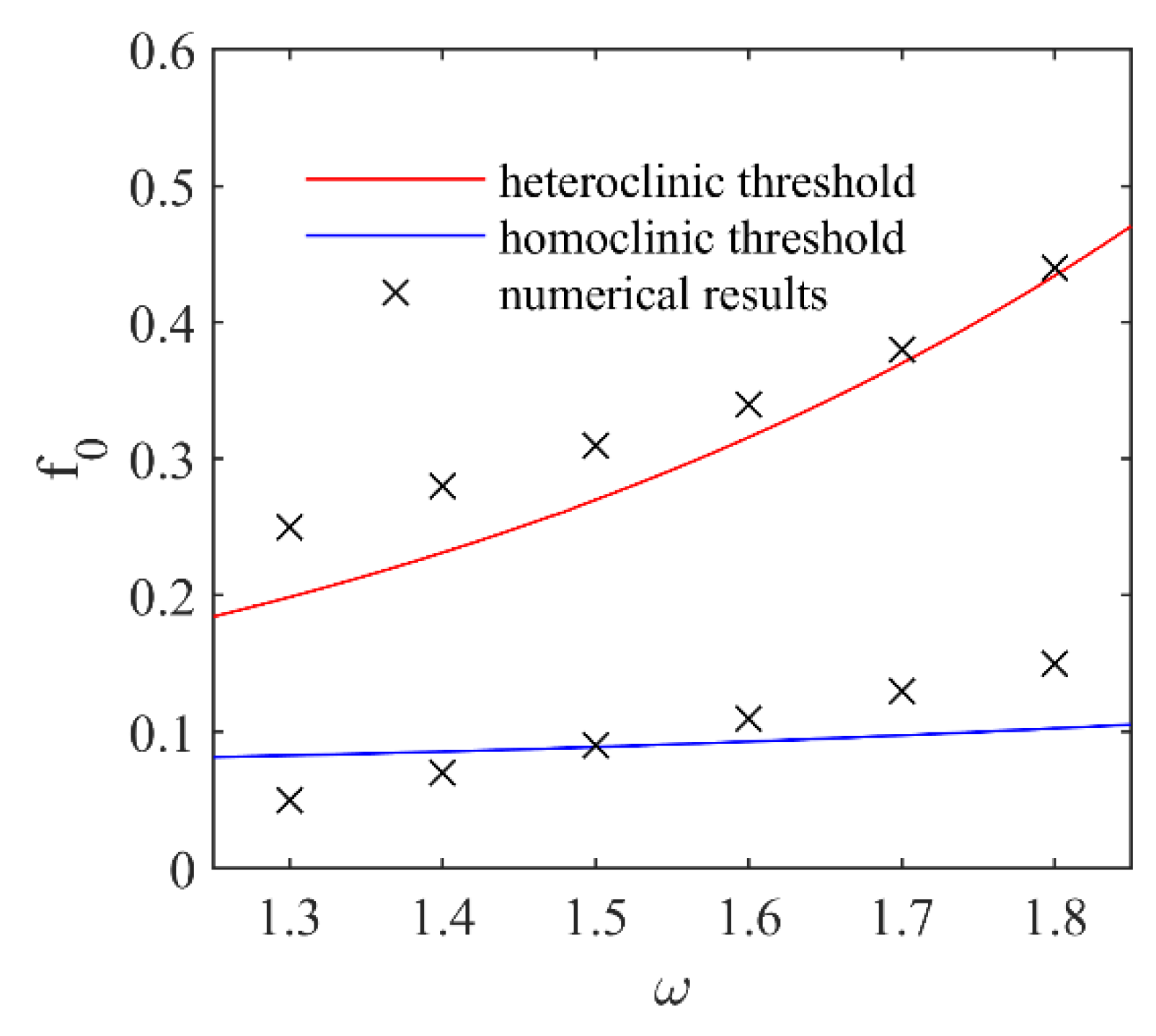
Based on Equations (54) and (55), i.e., the theoretical threshold of the dimensionless amplitude f 0 for homoclinic bifurcation and heteroclinic bifurcation, we present Figure 9 to show the variation of f 0 with the increase of excitation frequency ω. The blue curve and the red one represent the thresholds for homoclinic bifurcation and heteroclinic one, respectively. The numerical values of f 0 homo and f 0 h e t e r o are obtained at the points for the disappearance of two higher-amplitude intra-well attractors around nontrivial well centers and the occurrence of the inter-well attractor, respectively. For the purpose of energy harvesting, the former is unwanted for reducing jump, while the latter is desirable for inducing high-amplitude inter-well oscillation. Each numerical critical value of f 0 homo and f 0 h e t e r o is kept to two decimal places. We make sure that if f 0 is less than the numerical results f 0 homo or f 0 h e t e r o , the mentioned intra-well attractors will not disappear, or the inter-well periodic attractor will not appear, respectively. In Figure 9, the numerical results for the critical values of f 0 are in agreement with analytical ones, verifying the validity of the analysis. Figure 9 also demonstrates that the thresholds of the amplitude f 0 for homoclinic bifurcation and heteroclinic bifurcation will increase monotonically with ω. Comparatively, f 0 h e t e r o increases more rapidly than f 0 homo . In addition, Figure 9 shows that the lower the excitation frequency is, the lower threshold of the excitation amplitude to trigger inter-well oscillation will be, which will be helpful to harvest vibration energy.
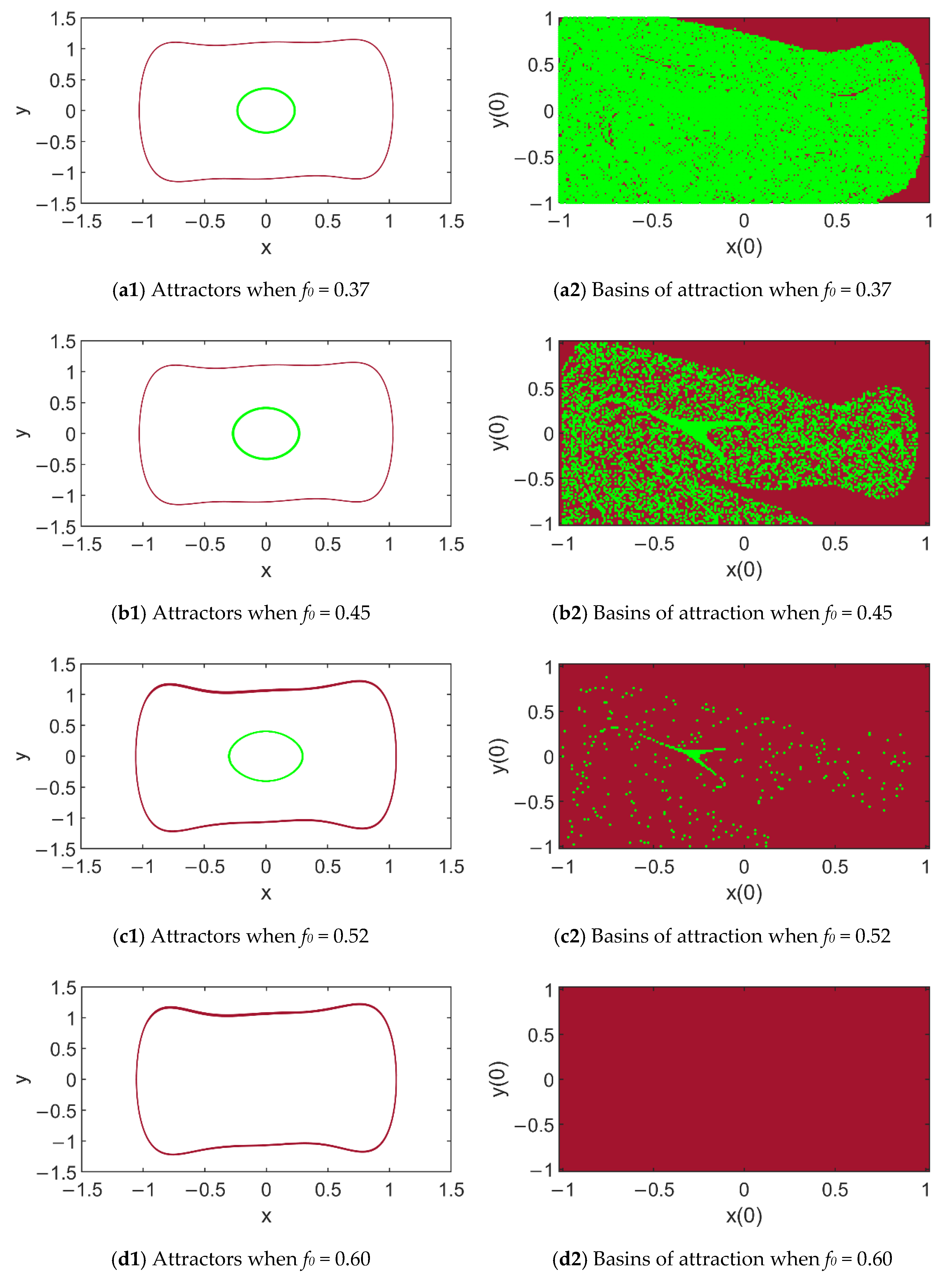
As f 0 continues to increase, the variation of the dynamical behaviors and their basins of attraction can be observed in Figure 10. For f 0 = 0.37, the basins of attraction of the inter-well attractor are enlarged and intermingled with the intra-well one, as can be observed from the grey region and grey dots scattered in the green region of Figure 10(a2). That means that the occurrence probability of inter-well oscillation and inter-well jump between the two attractors increases, which is surely good for energy harvesting. When f 0 increases to 0.45, the fractality of basins of attraction becomes more obvious, and the basins of attraction of the intra-well attractor are seriously eroded by the basin of the inter-well attractor (see the intermingled green and brown regions in Figure 10(b2)). For f 0 = 0.52, there is very little basin of attraction of the intra-well attractor left, showing that the intra-well attractor becomes a rare attractor. As f 0 reaches 0.60, the whole initial-condition plane is brown, illustrating that the inter-well response becomes globally attractive, and favorable for the structure to harvest energy.
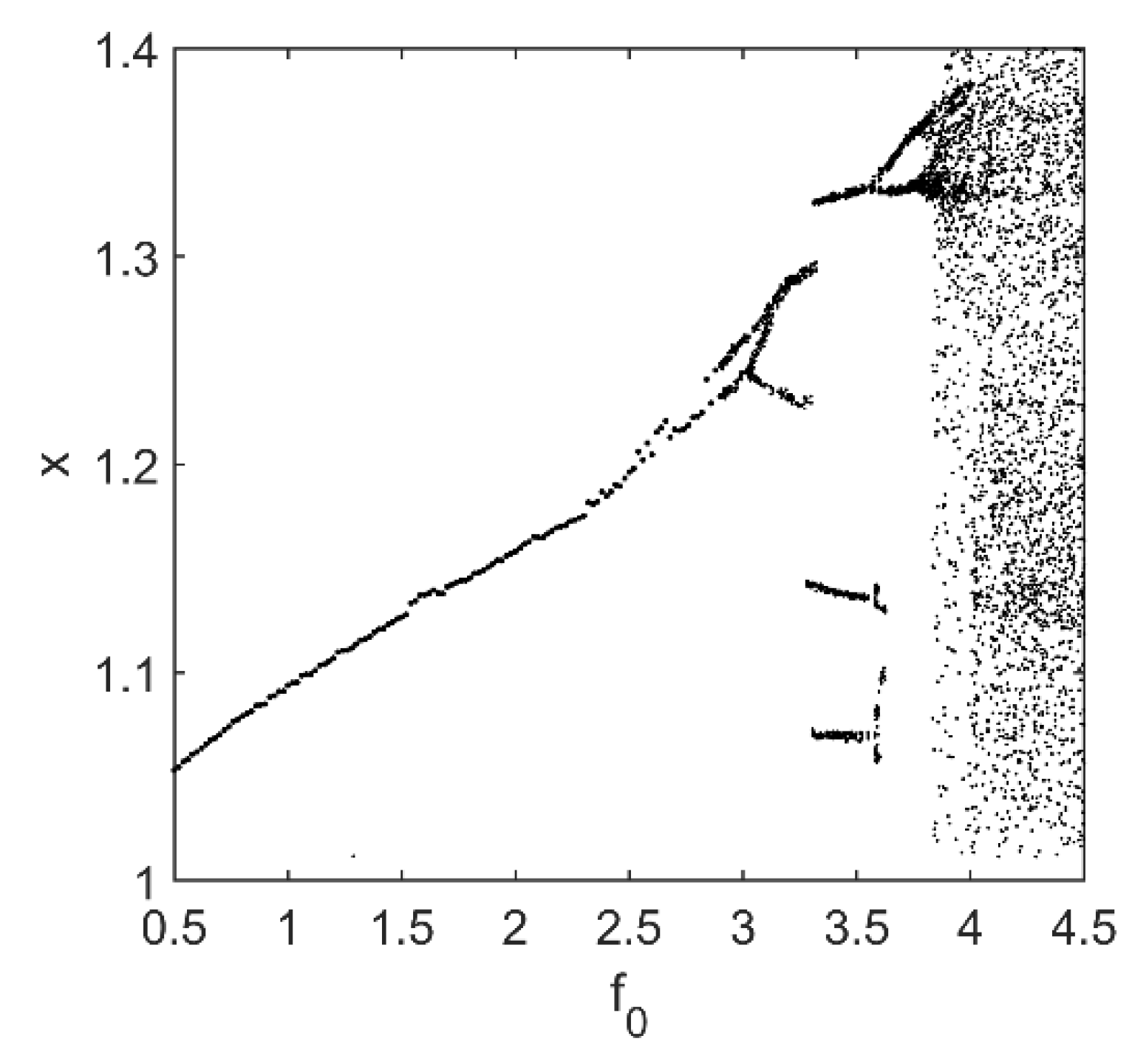
It is known that the Poincaré map is one of the most useful methods of investigating continuous-time nonlinear systems that involves a discretization technique [30]. For f0 continuing to increase, we present the bifurcation of the system (5) in the Poincaré map in Figure 11. Here, the points on the Poincaré map are collected from a cross-section at y = 0 and x > 0 in a sufficiently large time interval 5000 T 8000 to ensure that the response is stable. As can be observed, when f 0 
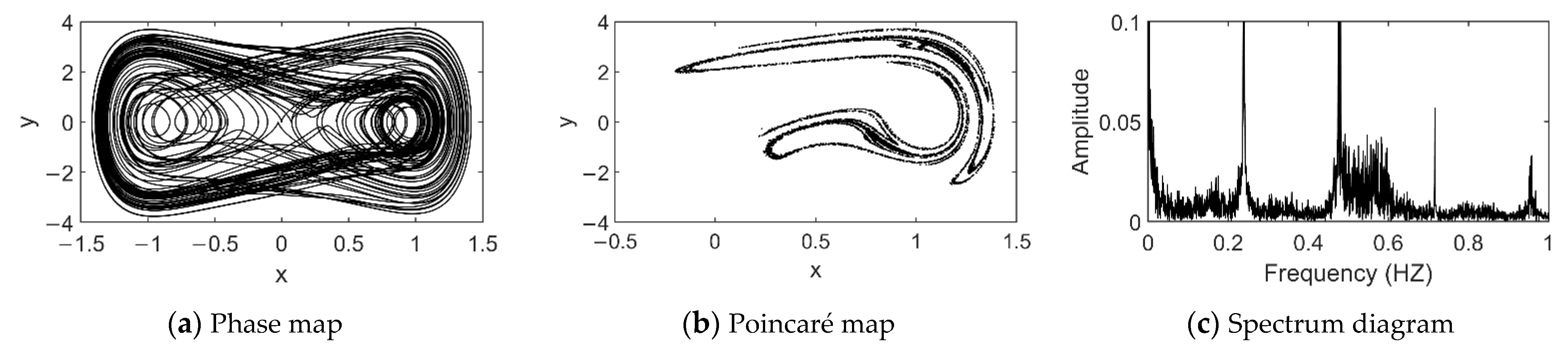
is more than 3.0, the system (5) evolves large-range inter-well chaotic motion through the routine of the period-doubling bifurcation. The chaotic vibration for f 0 = 4.2 is displayed via its phase map, Poincaré map and spectrum diagram in Figure 12. Note that points of the Poincaré map in Figure 12b are obtained from the cross-section at T = 2 n π satisfying 5000 T 8000 ; here n represents integers. It follows from Figure 11 and Figure 12 that global bifurcations finally lead to this large-range inter-well chaotic motion, which is unquestionably useful for energy harvesting.

5. Conclusions

It is well known that energy harvesters favor the appearance of complex dynamics. In this paper, bifurcations and complex dynamics of the electromechanical system of a piezoelectric energy harvester comprising a cantilever piezoelectric beam with an attached tip mass exposed to a harmonic tip force are investigated analytically and numerically.
First, the dimensionless ordinary differential equations governing the electromechanical system are obtained. The equilibrium bifurcation and stability have been investigated for the unperturbed system. The bifurcation sets of the equilibrium in parameter space have been constructed to demonstrate that the number and shapes of potential well depend on the coefficients of the polynomial form of the magnetic force: the smaller the penta power stiffness coefficient of nonlinear magnetic force is, the higher possibility for the occurrence of a triple potential well will be.
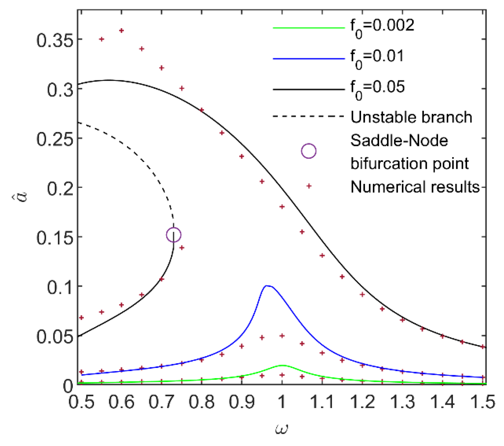
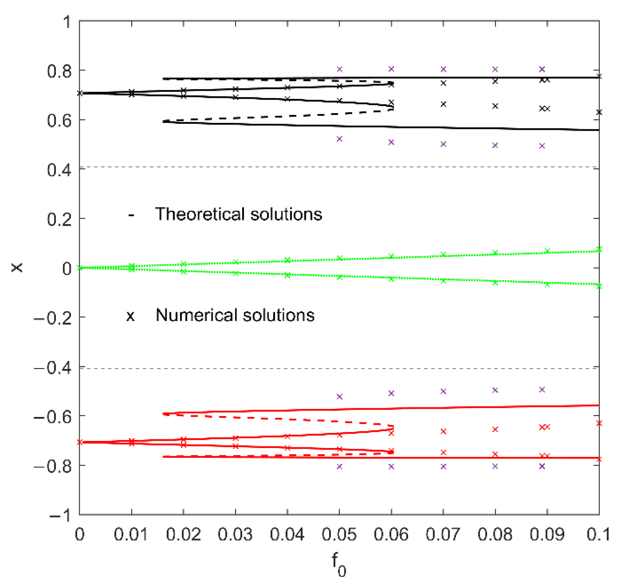
Then, fixing the physical parameters of the structure and varying the excitation amplitude and frequency, the case of a triple potential well is discussed. The Method of Multiple Scales is applied to provide analytical intra-well solutions. The oscillator is found to exhibit saddle-node bifurcation leading to bistable intra-well attractors around the same well center. Thus, the system may undergo four intra-well attractors or five intra-well attractors. The numerical integration method was then utilized to verify the solutions.
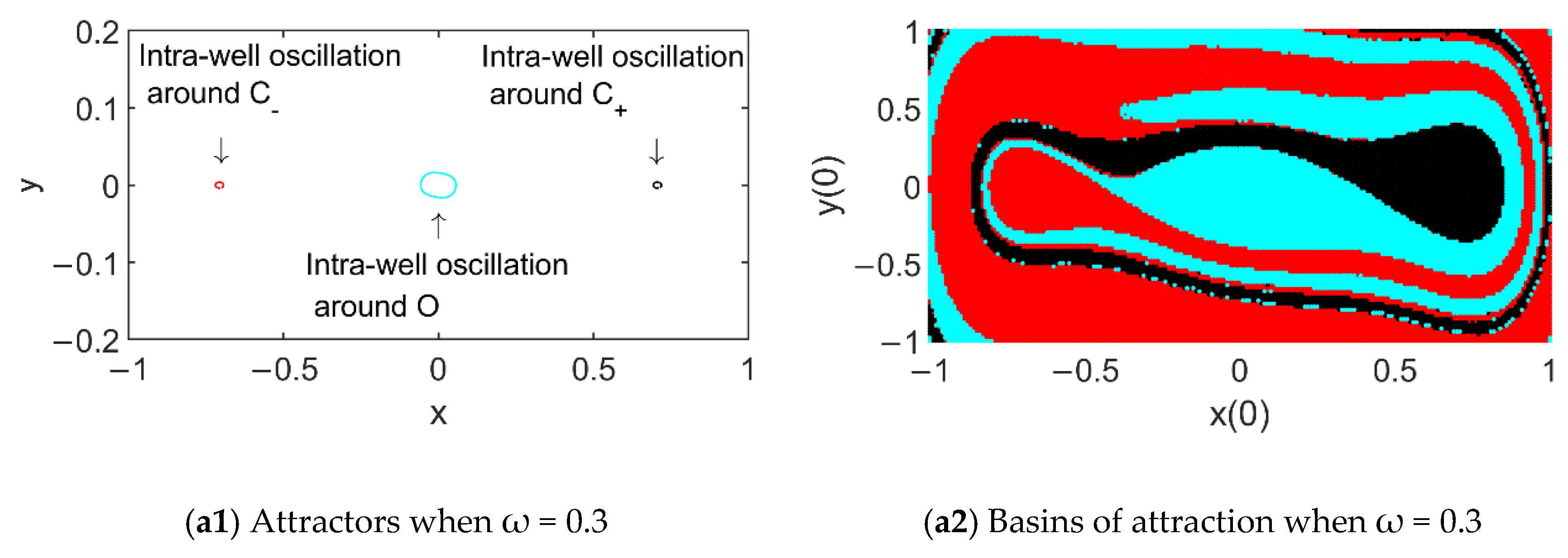
Consequently, we perform a detailed investigation of basins of attraction of multiple attractors that had still relatively little consideration in the literature. The basins of attraction are obtained by the point-mapping method. The numerical results further confirm the coexistence of these attractors, in good agreement with the theoretical ones, showing the validity of the analysis. It is found that in the regions with evidence of multistability basins of attraction with fractal structures occur quite frequently. We have also found extremely intermingled basins and rare attractors. It also reveals that for the excitation amplitude and frequency varying in the vicinity of saddle-node bifurcation points, the intra-well jump between the two intra-well attractors around the same well center is much easier to trigger than the inter-well jump among intra-well attractors around different well centers. The latter can be induced by a dramatic change of initial position or velocity. Both the two jumps are beneficial for energy harvesting.
Furthermore, analytical expressions for homoclinic orbits and heteroclinic orbits of the unperturbed system are derived. The Melnikov method is successfully employed to detect the analytical criteria for homoclinic bifurcation and heteroclinic bifurcation successively. These results obtained are verified by the numerical simulations in the form of phase maps, basins of attraction, bifurcation diagrams and Poincaré maps where fine agreement is achieved. It is found that the increase of the excitation amplitude can induce homoclinic bifurcation and heteroclinic bifurcation successively; the thresholds of the excitation amplitude for homoclinic bifurcation and heteroclinic bifurcation both increase monopoly with the increase of the excitation frequency. Homoclinic bifurcation induces the disappearance of the intra-well attractors around the nontrivial equilibria. An increase in the excitation amplitude can break the basins into discrete pieces or points. In contrast, heteroclinic bifurcation leads to the occurrence of a large-range jump between inter-well attractor and intra-well one, the globally attractive large-amplitude inter-well attractor, and eventually inter-well chaos through the routine of the period-doubling bifurcation. It implies that for the purpose of energy harvesting, homoclinic bifurcation is undesirable, while heteroclinic bifurcation is favorable.
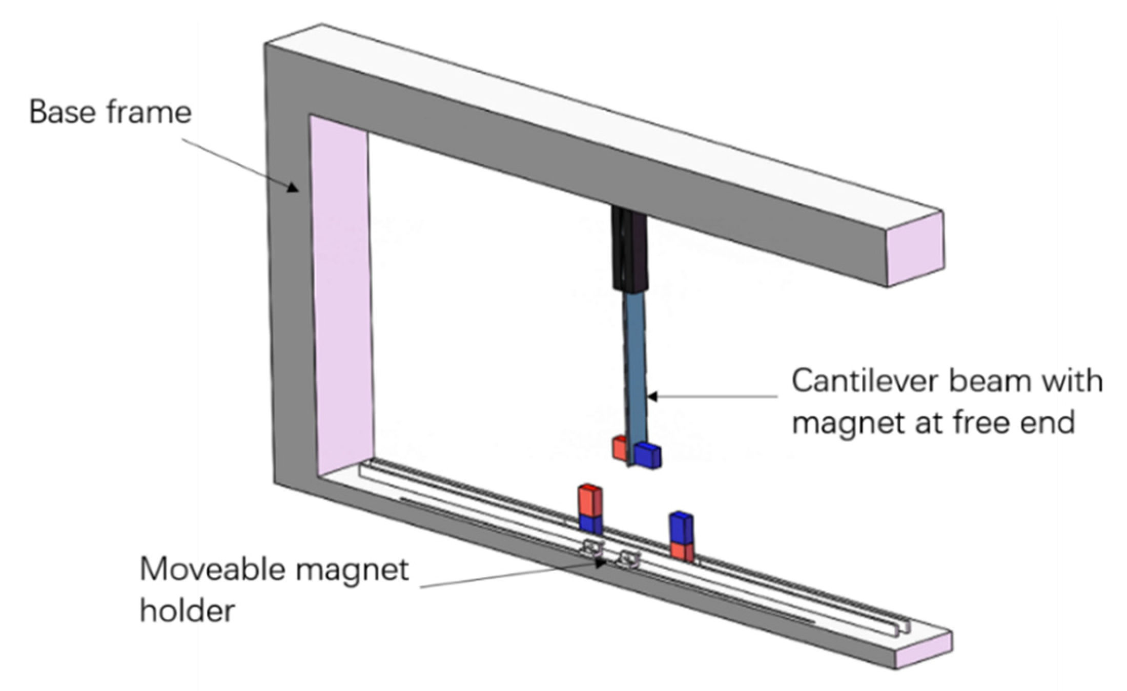
In this paper, the effect of the excitation amplitude, the excitation frequency as well as initial conditions on the nonlinear behavior of this triple-well piezoelectric energy harvester has been studied. Based on these investigations, the next steps will consist of designing an actual energy harvesting system featuring the calculated position of the equilibria, assessing the performance and optimizing the device. Hence, nonlinear magnetic interactions through the use of two magnets on a base interacting with a magnet at the free end of a cantilever beam can be considered. From an applicative point of view, a comparative analysis with moveable magnets on the base can be considered (see the structure in Figure 13).
It should be pointed out that the results in this paper are limited to the fixed physical properties of the structure. We have not considered the effect of physical properties on inducing the large-scale complex responses which can be beneficial for further optimization of triple-well energy harvesters. Jump phenomena, inter-well oscillation and large-range chaos that we have discussed in detail can make the structure under frequent strain. Considering the material characteristics of the piezoelectric generators, there may be brittles in piezo layers, leading to a challenge for the working lifespan of the devices. For better energy harvesting performance and reliability, these should be taken into account in theoretical study as well as experiments in practical application, which will be included in our future work.

Author Contributions

Conceptualization, H.S.; methodology, H.S.; software, Y.Z.; validation, H.S.; formal analysis, H.S.; investigation, Y.Z.; Writing-original draft preparation, Y.Z. and H.S.; writing-review and editing, H.S.; visualization, Y.Z.; supervision, H.S.; project administration, H.S.; funding acquisition, H.S. All authors have read and agreed to the published version of the manuscript.

Funding

This research was funded by the National Natural Science Foundation of China, grant number 11472176.

Institutional Review Board Statement

Not applicable.

Informed Consent Statement

Not applicable.

Data Availability Statement

Not applicable.

Acknowledgments

Huilin Shang acknowledges the support from the National Natural Science Foundation of China under grant number 11472176. The authors show their appreciation for the valuable comments from the reviewers on the manuscript.

Conflicts of Interest

The authors declare no conflict of interest.

References

  1. Wu, N.; Bao, B.; Wang, Q. Review on engineering structural designs for efficient piezoelectric energy harvesting to obtain high power output. Eng. Struct. 2021, 235, 112068. [Google Scholar] [CrossRef]
  2. Wei, C.; Jing, X. A comprehensive review on vibration energy harvesting: Modelling and realization. Renew. Sustain. Energy Rev. 2017, 74, 1–18. [Google Scholar] [CrossRef]
  3. Yang, T.; Cao, Q. Dynamics and high efficiency of a novel multi-stable energy harvesting system. Chaos Solitons Fractals 2020, 131, 109516. [Google Scholar] [CrossRef]
  4. Zhou, S.; Zuo, L. Nonlinear dynamic analysis of asymmetric tristable energy harvesters for enhanced energy harvesting. Commun. Nonlinear Sci. Numer. Simul. 2018, 61, 271–284. [Google Scholar] [CrossRef]
  5. Kumar, A.; Ali, S.F.; Arockiarajan, A. Exploring the benefits of an asymmetric monostable potential function in broadband vibration energy harvesting. Appl. Phys. Lett. 2018, 112, 233901. [Google Scholar] [CrossRef]
  6. Gu, Y.; Liu, W.; Zhao, C.; Wang, P. A goblet-like non-linear electromagnetic generator for planar multi-directional vibration energy harvesting. Appl. Energy 2020, 266, 114846. [Google Scholar] [CrossRef]
  7. Lallart, M.; Zhou, S.; Yang, Z.; Yan, L.; Li, K.; Chen, Y. Coupling mechanical and electrical nonlinearities: The effect of synchronized discharging on tristable energy harvesters. Appl. Energy 2020, 266, 114516. [Google Scholar] [CrossRef]
  8. Wang, C.; Zhang, Q.; Wang, W.; Feng, J. A low-frequency, wideband quad-stable energy harvester using combined nonlinearity and frequency up-conversion by cantilever-surface contact. Mech. Syst. Sig. Process. 2018, 112, 305–318. [Google Scholar] [CrossRef]
  9. Wang, C.; Zhang, C.; Wang, W. Low-frequency wideband vibration energy harvesting by using frequency up-conversion and quin-stable nonlinearity. J. Sound Vib. 2017, 399, 169–181. [Google Scholar] [CrossRef]
  10. Zhou, S.; Cao, J.; Inman, D.; Lin, J.; Liu, S.; Wang, Z. Broadband tristable energy harvester: Modeling and experiment verification. Appl. Energy 2014, 133, 33–39. [Google Scholar] [CrossRef]
  11. Li, H.; Ding, H.; Chen, L. Chaos threshold of a multistable piezoelectric energy harvester subjected to wake-galloping. Int. J. Bifurc. Chaos 2019, 29, 1950162. [Google Scholar] [CrossRef]
  12. Naseer, R.; Dai, H.; Abdelkefi, A.; Wang, L. Comparative study of piezoelectric vortex-induced vibration-based energy harvesters with multi-stability characteristics. Energies 2019, 13, 71. [Google Scholar] [CrossRef]
  13. Yang, X.; Wang, C.; Lai, S. A magnetic levitation-based tristable hybrid energy harvester for scavenging energy from low-frequency structural vibration. Eng. Struct. 2020, 221, 110789. [Google Scholar] [CrossRef]
  14. Wang, C.; Lai, S.; Wang, J.; Fenf, J.-J.; Ni, Y.-Q. An ultra-low-frequency, broadband and multi-stable tri-hybrid energy harvester for enabling the next-generation sustainable power. Appl. Energy 2021, 291, 116825. [Google Scholar] [CrossRef]
  15. Rezaei, M.; Khadem, E.S.; Friswell, I.M. Energy harvesting from the secondary resonances of a nonlinear piezoelectric beam under hard harmonic excitation. Meccanica 2020, 55, 1463–1479. [Google Scholar] [CrossRef]
  16. Chen, X.; Zhang, X.; Wang, L.; Chen, L. An arch-linear composed beam piezoelectric energy harvester with magnetic coupling: Design, modeling and dynamic analysis. J. Sound Vib. 2021, 513, 116394. [Google Scholar] [CrossRef]
  17. Ju, Y.; Li, Y.; Tan, J.; Zhao, Z.; Wang, G. Transition mechanism and dynamic behaviors of a multi-stable piezoelectric energy harvester with magnetic interaction. J. Sound Vib. 2021, 501, 116074. [Google Scholar] [CrossRef]
  18. Cao, J.; Zhou, S.; Inman, D.J.; Chen, Y. Chaos in the fractionally damped broadband piezoelectric energy generator. Nonlinear Dyn. 2014, 80, 1705–1719. [Google Scholar] [CrossRef]
  19. Lallart, M.; Zhou, S.; Yan, L.; Yang, Z.; Chen, Y. Tailoring multistable vibrational energy harvesters for enhanced performance: Theory and numerical investigation. Nonlinear Dyn. 2019, 96, 1283–1301. [Google Scholar] [CrossRef]
  20. Tékam, G.T.O.; Kuimy, C.K.; Woafo, P. Analysis of tristable energy harvesting system having fractional order viscoelastic material. Chaos 2015, 25, 191–206. [Google Scholar]
  21. Karličić, D.; Chatterjee, T.; Cajić, M.; Adhikari, S. Parametrically amplified Mathieu-Duffing nonlinear energy harvesters. J. Sound Vib. 2020, 488, 115677. [Google Scholar] [CrossRef]
  22. Barbosa, W.; Paula, A.; Savi, M.; Inman, D. Chaos control applied to piezoelectric vibration-based energy harvesting systems. Eur. Phys. J. Spec. Top. 2015, 224, 2787–2801. [Google Scholar] [CrossRef]
  23. Chen, Z.; Guo, B.; Cheng, C.; Shi, H.; Yang, Y. Chaotic dynamics-based analysis of broadband piezoelectric vibration energy harvesting enhanced by using nonlinearity. Shock Vib. 2016, 2016, 3584740. [Google Scholar] [CrossRef]
  24. Zhang, J.; Li, X.; Feng, X.; Li, R.; Dai, L.; Yang, K. A novel electromagnetic bistable vibration energy harvester with an elastic boundary: Numerical and experimental study. Mech. Syst. Signal Process. 2021, 160, 107937. [Google Scholar] [CrossRef]
  25. Fu, Y.; Ouyang, H.; Davis, R. Nonlinear structural dynamics of a new sliding-mode triboelectric energy harvester with multistability. Nonlinear Dyn. 2020, 100, 1941–1962. [Google Scholar] [CrossRef]
  26. Zhu, Y.; Shang, H. Multistability of the vibrating system of a micro resonator. Fractal Fract. 2022, 6, 141. [Google Scholar] [CrossRef]
  27. Chudzik, A.; Perlikowski, P.; Stefanski, A.; Kapitaniak, T. Multistability and rare attractors in Van der Pol-Duffing Oscillator. Int. J. Bifurc. Chaos 2011, 21, 1907–1912. [Google Scholar] [CrossRef]
  28. Ashhab, M.; Salapaka, M.; Dahleh, M.; Mezić, I. Melnikov-based dynamical analysis of microcantilevers in scanning probe microscopy. Nonlinear Dyn. 1999, 20, 197–220. [Google Scholar] [CrossRef]
  29. Shang, H. Pull-in instability of a typical electrostatic MEMS resonator and its control by delayed feedback. Nonlinear Dyn. 2017, 90, 171–183. [Google Scholar] [CrossRef]
  30. Stephen, W.; David, M. Introduction to applied nonlinear dynamical systems and chaos. Comput. Phys. 1990, 4, 563. [Google Scholar]
Figure 1. Simplified diagram of a tristable piezoelectric cantilever energy harvester.
Mathematics 10 02894 g001
Figure 2. Orbits of the unperturbed system (6) under different values of k1 and k2.
Mathematics 10 02894 g002
Figure 3. Variation of the amplitude of periodic solutions near (0, 0) with the change of ω.
Mathematics 10 02894 g003
Figure 4. Evolution of attractors and their basins of attraction with the increase of ω for f0 = 0.05.
Mathematics 10 02894 g004aMathematics 10 02894 g004b
Figure 5. Variation of the amplitude of periodic solution near ( ± x c , 0) with the change of ω.
Mathematics 10 02894 g005
Figure 6. Variation of the periodic solutions with the amplitude of f0 when ω = 1.5.
Mathematics 10 02894 g006
Figure 7. Evolution of attractors and their basins of attraction with the increase of f0 for ω = 1.5.
Mathematics 10 02894 g007
Figure 8. Sequences of attractors and their basins of attraction for f0 ranging from 0.089 to 0.31.
Mathematics 10 02894 g008aMathematics 10 02894 g008b
Figure 9. f 0 homo and f 0 h e t e r o of system (5) versus the excitation frequency ω.
Mathematics 10 02894 g009
Figure 10. Sequences of attractors and their basins of attraction for f0 ranging from 0.37 to 0.60.
Mathematics 10 02894 g010
Figure 11. Bifurcation diagram under different values of f0.
Mathematics 10 02894 g011
Figure 12. Chaos of the system (5) for f0 = 4.2.
Mathematics 10 02894 g012
Figure 13. Possible experimental implementation.
Mathematics 10 02894 g013
Table 1. Parameters of systems (1) and (5).
ParameterSymbol
Equivalent mass of the proof mass (kg)m
Equivalent damping of the piezoelectric beam (N·s/m)c
Linear stiffness (N/m) a 1
Cubic stiffness term (N/m3) a 2
Penta power stiffness term (N/m5) a 3
Electromechanical coupling coefficient (N/V)kem
Amplitude of the external excitation (N)F
Frequency of the external excitation (HZ) Ω
Equivalent capacitance of piezoelectric layers (F)cp
Load resistance (kΩ) r l
Length of substrate layer (mm)L
Initial voltage of energy harvesting circuits (V) V 0
Timet
Tip displacement of the harvester at time t X ( t )
Voltage at time t V ( t )
Natural frequency of the dynamical system ω 0
Dimensionless linear damping term μ
Dimensionless cubic stiffness term k 1
Dimensionless penta power stiffness term k 2
Dimensionless electromechanical coupling term η
Dimensionless excitation amplitude f 0
Dimensionless excitation frequency ω
Dimensionless stiffness term of the coil current system γ
Dimensionless electromechanical damping coefficient term β
Dimensionless timeT
Dimensionless displacement at time Tx
Dimensionless voltage at time Tv
Publisher’s Note: MDPI stays neutral with regard to jurisdictional claims in published maps and institutional affiliations.

