An Unconditionally Stable Integration Method for Structural Nonlinear Dynamic Problems

Abstract

This paper presents an unconditionally stable integration method, which introduces a linearly implicit algorithm featuring an explicit displacement expression. The technique that is being considered integrates one Newton iteration into the mean acceleration method. The stability of the proposed algorithm in solving equations of motion containing nonlinear restoring force and nonlinear damping force is analyzed using the root locus method. The objective of this investigation was to assess the accuracy and consistency of the proposed approach in contrast to the Chang method and the CR method. This is achieved by analyzing the dynamic response of three distinct structures: a three-layer shear structure model outfitted with viscous dampers, a three-layer shear structure model featuring metal dampers, and an eight-story planar frame structure. Empirical evidence indicates that the algorithm in question exhibits a notable degree of precision and robustness when applied to nonlinear dynamic problem-solving.

1. Introduction

With the continuous development of viscous damping materials, viscoelastic materials, and metallic materials, more and more new types of dampers with greater energy dissipation capacity and deformation capacity have emerged [1,2,3]. The complexity of structural nonlinearities is heightened by the incorporation of diverse types of dampers [4,5]. The research significance of numerical integration methods has been reaffirmed in order to address the task of solving discrete motion equations. Time integration algorithms, often known as TIAs, are very popular in the field of structural dynamics owing to the simplicity with which they can be programmed [6,7].

TIAs have been developed for decades and have a considerable number of research results. The present study discusses various methods that are commonly used in the field. These methods include the Newmark family of integration algorithms [8], Wilson-θ method [9], Park method [10], HHT-α method [11], WBZ-α method [12], CH-α method [13,14], composite implicit time integration method [15], OS method [16], the IHOA family of methods [17], the MIHOA family of algorithms [18], B-sample method [19], implicit integration method for dislocation dynamics [20], and three-parameter GS4-2 algorithm [21,22]. The categorization of TIAs is commonly recognized as comprising two distinct types, namely explicit and implicit, as evidenced by various scholarly sources [23,24]. Explicit algorithms are defined as assuming that the solution to the problem is already known, and the calculation of new response values within each step only requires the use of the quantities already obtained in the previous steps. Thus, the algorithms can be performed directly step by step, making the calculation process straightforward and simple, and less time-consuming [15]. The algorithm that is explicitly used is typically subject to conditional stability, as noted by various authors [25,26,27]. Specifically, the numerical solution is stable only if the proportion between the integration step and the intrinsic period of the structure, Δt/Tn, is below a certain threshold [28]. In contrast to explicit algorithms, in implicit algorithms, the expression that gives the new value for the current step contains one or more values related to the current step, so the predicted value of the desired quantity must be assumed and then the predicted value is improved by continuous iterations [18,29].

As per the preceding literature, explicit and implicit integration algorithms both have their benefits and drawbacks, so methods that can combine the computational efficiency of explicit integration algorithms and the higher numerical stability of implicit integration algorithms need to be developed. Linearly implicit integration techniques have been devised to integrate a pre-determined number of iterations into the implicit algorithm’s expression. This results in an explicit format for the algorithm’s expression [30,31,32]. The novel approach enhances computational efficiency without compromising the original implicit methods’ stability.

Recently, linearly implicit TIAs have been proposed by many researchers. The Chang method with second-order accuracy based on the average acceleration method by introducing two control parameters was derived by Taiwanese scholar S. Y. Chang in 2002 [32,33]. The algorithm in question is deemed unconditionally stable when applied to linear problems. It has been observed that a notable computational discrepancy arises when endeavoring to solve motion equations that integrate nonlinear restoring forces for structures that undergo substantial alterations in their condition, whereby stiffness is significantly modified [34,35]. Chen and Ricles introduced a linear implicit numerical integration algorithm, known as the CR method, which achieves second-order accuracy through the application of discrete control theory [36]. This approach is distinct from the Chang method. When calculating the equations of motion for structures with significant variations in stiffness over time, the CR technique also suffers from significant computational mistakes due to the presence of nonlinear restoring force [34,37,38,39]. The Rosenbrock technique is a linear implicit integration method that may be generated by embedding a single Newton iteration in an implicit Runge–Kutta algorithm [40]. This approach keeps both the original as well as the result of the embedded iteration. The Rosenbrock technique is a first-order numerical method that requires the reduction of equation order when applied to structural dynamic issues. It will increase the amount of work that needs to be done on the computer.

The aim of the present work is to introduce a novel methodology for addressing nonlinear structural problems by integrating the Newton iteration technique employed in the Rosenbrock method into the mean acceleration method. This results in the development of a linearly implicit method. The algorithm under consideration is subjected to analysis through the utilization of the root trajectory technique. Subsequently, the precision of the aforementioned method is scrutinized through the implementation of three numerical simulations. The simulations conducted in this study involve three distinct structural models, namely a three-layer shear structure model equipped with viscous dampers, a three-layer shear structure model featuring metal dampers, and an eight-layer planar frame structure. A comparative analysis was conducted to evaluate the precision of the suggested algorithm in relation to the Chang and CR techniques. The findings indicate that the algorithm put forth demonstrates significant precision and enhanced consistency when applied to nonlinear dynamic issues.

2. Introduction of Several Integration Algorithms

2.1. Newmark-β Method

The Newmark-β algorithm has been extensively employed for solving second-order motion equations [6,41]. The motion equation for a multi-degree-of-freedom (MDoF) mechanism with nonlinear restoring and damping forces can be formulated as follows:

$$Ma+h(v)+f(d)=g(t),$$

(1)

where $\mathit{M}$ represents the mass matrix, $\mathit{h}(\mathit{v})$ indicates the nonlinear force vector associated with velocity $\mathit{v}$, $\mathit{f}(d)$ is the nonlinear force associated with displacement $d$, and $\mathit{g}(t)$ denotes the external force vector.

The Newmark-β method initially postulates the fluctuation of acceleration within a timeframe of arbitrary duration. Subsequently, the initial state quantity of motion at the onset of the time step is utilized as the initial value. The expressions for velocity and displacement at the conclusion of the time step are then obtained in the following forms:

$$v_{n+1}=v_n+\Delta t((1-\gamma ){\alpha }_n+\gamma a_{n+1}),0\le \gamma \le 1,$$

(2)

$$d_{n+1}=d_n+\Delta t{v}_n+\frac{1}{2}\Delta t^2((1-2\beta )a_n+2\beta a_{n+1}),0\le \beta \le \frac{1}{2},$$

(3)

when $\gamma =1/2$ and $\beta =1/4$, the consistent acceleration approach (second-order precision, unconditional stability, and implicit format) is maintained.

2.2. Chang Method

The author, S. Y. Chang, put forward a TIA that is implicitly formulated and possesses unconditional stability. This algorithm is an extension of the mean acceleration method [32]. The Chang method incorporates two parameters, denoted as ${\beta }_1$ and ${\beta }_2$, into the displacement expression, respectively, which can be mathematically expressed as follows:

$$v_{n+1}=v_n+{\alpha }_1{a}_n\Delta t,$$

(4)

$$d_{n+1}=d_n+v_n\Delta t+{\alpha }_2{a}_n\Delta t^2,$$

(5)

in the formula,

$${\beta }_1={[1+\frac{1}{2}{M}^{-1}C\Delta t+\frac{1}{4}{M}^{-1}{K}_0\Delta t^2]}^{-1}[1+\frac{1}{2}{M}^{-1}C\Delta t],$$

(6)

$${\beta }_2=\frac{1}{2}{[1+\frac{1}{2}{M}^{-1}C\Delta t+\frac{1}{4}{M}^{-1}{K}_0\Delta t^2]}^{-1},$$

(7)

where ${\mathit{K}}_0$ denotes the initial stiffness matrices of the structure being analyzed.

2.3. CR Method

Chen and Ricles introduced a method that is unconditionally stable and relies on discrete control theory, as proposed in their work [36]. The CR method incorporates two parameters, ${\alpha }_1$ and ${\alpha }_2$, into the expressions for velocity and displacement. These expressions are formulated as follows:

$$v_{n+1}=v_n+{\alpha }_1{a}_n\Delta t,$$

(8)

$$v_{n+1}=v_n+{\alpha }_1{a}_n\Delta t,$$

(9)

in the formula,

$${\alpha }_1={\alpha }_2=4M{\left(4M+2C\Delta t+K_0\Delta t^2\right)}^{-1}.$$

(10)

2.4. Rosenbrock Integration Method and Implicit Algorithm with an Embedded Newton Iteration of Velocity

A single Newton iteration is included in the implicit Runge–Kutta technique in Rosenbrock’s approach, making it a standard linearly implicit numerical integration procedure. This technique avoids iterative computations while maintaining the same level of consistency as the classic Runge–Kutta method [40,42]. Writing the motion equation in a lower-order Hamiltonian form is the first step in using the Rosenbrock approach:

$$\dot{\mathit{y}}=\mathit{F}\left(y,t\right)=\left\{\begin{array}{c}v\\ M^{(-1)}(g(t)-h(v)-f(d))\end{array}\right\},$$

(11)

where $\mathit{y}=\left\{\begin{array}{c}\mathit{u}\\ \mathit{v}\end{array}\right\}$ defines the state vector. The solution of Equation (11) is the mean of the s-stage. The Rosenbrock method is given by

$$y_{n+1}=y_n+{\displaystyle {\sum }_{i=1}^s{b}_i{k}_i},$$

(12)

$$k_i={\left[1-\gamma J\Delta t\right]}^{-1}\left(F\left(t_n+{\alpha }_i\Delta t,y_n+{\displaystyle {\sum }_{j=1}^{i-1}{\alpha }_{ij}{k}_j}\right)+J{\displaystyle {\sum }_{j=1}^{i-1}{\gamma }_{ij}{k}_j}\right)\Delta t,$$

(13)

where ${\alpha }_i={\displaystyle {\sum }_{j=1}^{i-1}{\alpha }_{ij}}$, ${\gamma }_{ij}$ and $b_i$ denote the algorithm parameters, and $\mathit{J}$ presents the Jacobian matrix, its definition being as follows:

$$J=\frac{\partial F}{\partial y}.$$

(14)

The Rosenbrock method requires updating $J$ at the outset of each step.

The present discussion aims to elucidate the approach of incorporating the Newton iteration technique in a comprehensive manner. To this end, the first-order Rosenbrock method has been employed as an exemplar.

$$k_1={\left[1-\gamma J\Delta t\right]}^{-1}F(y_n,t_n)\Delta t,y_{n+1}=y_n+b_1{k}_1.$$

(15)

The derivation of Equation (15) utilizing the Newton iteration principle is presented below.

To begin, the first-order Runge–Kutta algorithm has the following expression:

$$y_{n+1}=y_n+(1-\gamma )F(y_n,t_n)\Delta t+\gamma F(y_{n+1},t_{n+1})\Delta t.$$

(16)

The above formula can be transformed:

$$y_n+(1-\gamma )F({\mathit{y}}_n,t_n)\Delta t+\gamma F(y_{n+1},t_{n+1})\Delta t-y_{n+1}=0.$$

(17)

Assume the left side of Equation (17) to be $p(x)$, and replace $y_{n+1}$ with $x$ in the formula:

$$p(x)=y_n+\left[(1-\gamma )F(y_n,t_n)+\gamma F(x,t_{n+1})\right]\Delta t-x=0.$$

(18)

Determine the derivative of to $x$:

$$p^{\prime }(x)=\gamma \Delta t{F}^{\prime }(x,t_{n+1})-1.$$

(19)

Suppose the initial value $x^{\left(0\right)}$ to be $y_n$. Incorporating Equations (18) and (19) into a single Newton iteration equation yields:

$$p^{\prime }(x)=\gamma \Delta t{F}^{\prime }(x,t_{n+1})-1,$$

(20)

where $J={\partial \mathit{F}/\partial \mathit{x}|}_{x=y_n}$ stands for the Jacobian matrix at time $t_n$.

Typically, in the iterative process, it is assumed that the initial value of $y_n$ is $y_{n+1}$. The integration step utilized in the integration procedure necessitates a sufficiently brief duration, such that the disparity between $y_n$ and $y_{n+1}$ is minimal, and their gradients can be estimated as being equivalent. Thus, it is typically the case that a single iteration is sufficient to meet specific accuracy criteria.

Driven by the strategy of the Rosenbrock method, one Newton iteration is introduced into the average acceleration method.

The incorporation of a Newton iteration into the average acceleration method was motivated by the Rosenbrock method strategy, as reported by reference [43].

The formula for calculating the average acceleration technique in a multiple MDOF system is:

$$d_{n+1}=d_n+\Delta t{v}_n+\frac{1}{4}\Delta t^2{a}_n+\frac{1}{4}\Delta t^2{a}_{n+1},$$

(21)

$$v_{n+1}=v_n+\frac{1}{2}\Delta t{a}_n+\frac{1}{2}\Delta t{a}_{n+1}.$$

(22)

Equations (21) and (22) can be used to depict the acceleration term ${\mathit{a}}_{n+1}$ and the displacement term $d_{n+1}$ expressed as a function of the velocity term ${\mathit{v}}_{n+1}$ as the fundamental state vector:

$$a_{n+1}=2\frac{v_{n+1}-v_n}{\Delta t}-a_n,$$

(23)

$$d_{n+1}=\Delta t\frac{v_{n+1}+v_n}{2}+d_n.$$

(24)

Equations (23) and (24) are substituted into Equation (21),

$$M\left(2\frac{v_{n+1}-v_n}{\Delta t}-a_n\right)+h(v_{n+1})+f\left(\Delta t\frac{v_{n+1}+v_n}{2}+d_n\right)=g_{n+1}.$$

(25)

The expressions of $d_{n+1}$, ${\mathit{v}}_{n+1}$, and ${\mathit{a}}_{n+1}$ can be obtained:

$$d_{n+1}={\overline{\mathit{d}}}_{n+1}+\frac{\Delta t}{2}\Delta {\mathit{v}}_n,$$

(26)

$$v_{n+1}=v_n+\Delta v_n,$$

(27)

$$a_{n+1}=-a_n+\frac{2}{\Delta t}\Delta v_n.$$

(28)

Equations (26)–(28) are the explicit recursive format of the new algorithm. The determination of the velocity increment $\Delta v_n$ is of utmost importance. Upon solving for it, the values of $d_{n+1}$, $v_{n+1}$, and $a_{n+1}$ can be obtained [43].

3. Derivation of a Novel Linearly Implicit Algorithm

The incorporation of a Newton iteration into the mean acceleration technique is informed by the Rosenbrock method’s approach, which provides a basis for the method’s execution. It is possible to create a novel linearly implicit technique by implementing the embedded Newton iteration and utilizing the displacement term as the iteration parameter.

When dealing with an MDoF system, if the restoring and damping forces exhibit nonlinearity, the motion equations that govern the system at a given time $t_{n+1}$ could be mathematically represented as follows:

$$M{a}_{n+1}+h(v_{n+1})+f(d_{n+1})=g_{n+1},$$

(29)

where $d_{n+1}$, $v_{n+1}$, and $a_{n+1}$ stand for the displacement, velocity, and acceleration response vectors at $t_{n+1}$, respectively, and $g_{n+1}$ stands for the external force vector at time $t_{n+1}$.

Equations (21) and (22) can be expressed in terms of the variable $d_{n+1}$ to denote the velocity term $v_{n+1}$ and the acceleration term $a_{n+1}$:

$$v_{n+1}=2\frac{d_{n+1}-d_n}{\Delta t}-v_n,$$

(30)

$$a_{n+1}=4\frac{d_{n+1}-d_n}{\Delta t^2}-\frac{4}{\Delta t}{v}_n-a_n.$$

(31)

Equations (30) and (31) are substituted into Equation (21), resulting in

$$M\left(4\frac{d_{n+1}-d_n}{\Delta t^2}-\frac{4}{\Delta t}{v}_n-a_n\right)+h(2\frac{d_{n+1}-d_n}{\Delta t}-v_n)+f\left(d_{n+1}\right)=g_{n+1}.$$

(32)

The above formula can be transformed as follows:

$$M\left(4\frac{d_{n+1}-d_n}{\Delta t^2}-\frac{4}{\Delta t}{v}_n-a_n\right)+h(2\frac{d_{n+1}-d_n}{\Delta t}-v_n)+f\left(d_{n+1}\right)-g_{n+1}=0.$$

(33)

Suppose the unknown displacement ${\mathit{d}}_{n+1}$ is $\mathit{x}$, and the left side of Equation (33) could be expressed as a function of $\mathit{x}$:

$$p(x)=M\left(4\frac{x-d_n}{\Delta t^2}-\frac{4}{\Delta t}{v}_n-a_n\right)+h(2\frac{x-d_n}{\Delta t}-v_n)+f\left(x\right)-g_{n+1}.$$

(34)

To perform one Newton iteration, assume the beginning value of $\mathit{x}$ as $d_n$, and the corresponding value of $p(x)$ at $\mathit{x}=d_n$ can be computed as:

$$p(d_n)=M\left(-a_n-\frac{4}{\Delta t}{v}_n\right)+h(-v_n)+f(d_n)-g_{n+1}.$$

(35)

In such a case, when $x=d_n$, the first-order partial derivative of $p(x)$ with respect to $x$ may be calculated as follows:

$${\frac{\partial p(x)}{\partial x}|}_{\mathit{x}=d_n}=\frac{4}{\Delta t^2}M+{\frac{2}{\Delta t}\frac{\partial h(v)}{\partial v}|}_{v=-v_n}x+{\frac{\partial f(x)}{\partial x}|}_{x=d_n}.$$

(36)

Using one Newton iteration, $d_{n+1}$, the solution of $p(x)=0$ is as follows:

$$d_{n+1}=d_n-{\left({\frac{\partial p(x)}{\partial x}|}_{x=d_n}\right)}^{-1}p(d_n).$$

(37)

By substituting Equations (35) and (36) into Equation (37), the increment of displacement, represented by $\Delta d_n$, can be mathematically formulated as

$$\Delta d_n=-{\left(\frac{4}{\Delta t^2}M+\frac{2}{\Delta t}{\frac{\partial h(v)}{\partial v}|}_{v=-v_n}+{\frac{\partial f(x)}{\partial x}|}_{x=d_n}\right)}^{-1}\left(M\left(-a_n-\frac{4}{\Delta t}{v}_n\right)+h(-v_n)+f(d_n)-g_{n+1}\right).$$

(38)

By inserting Equation (38) into Equations (21) and (22), one can derive the formulas for $v_{n+1}$ and $a_{n+1}$ as:

$$v_{n+1}=-v_n+\frac{2}{\Delta t}\Delta d_n,$$

(39)

$$a_{n+1}=\frac{4}{\Delta t^2}\Delta d_n-\frac{4}{\Delta t}{v}_n-a_n,$$

(40)

$$d_{n+1}=\Delta d_n+d_n.$$

(41)

The explicit recursive format of the new algorithm is represented by Equations (39)–(41). The resolution of the displacement increment $\Delta {\mathit{v}}_n$ is of utmost importance. Upon resolving $\Delta d_n$, the subsequent values of $d_{n+1}$, $v_{n+1}$, and ${\mathit{a}}_{n+1}$ can be derived.

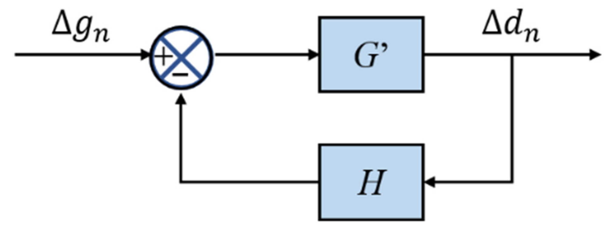
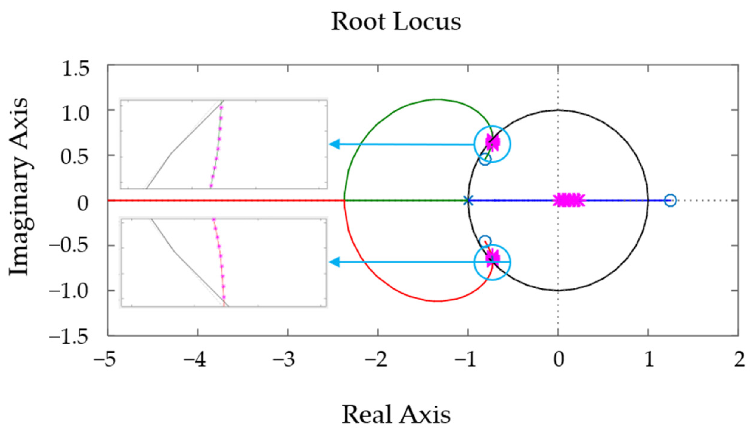
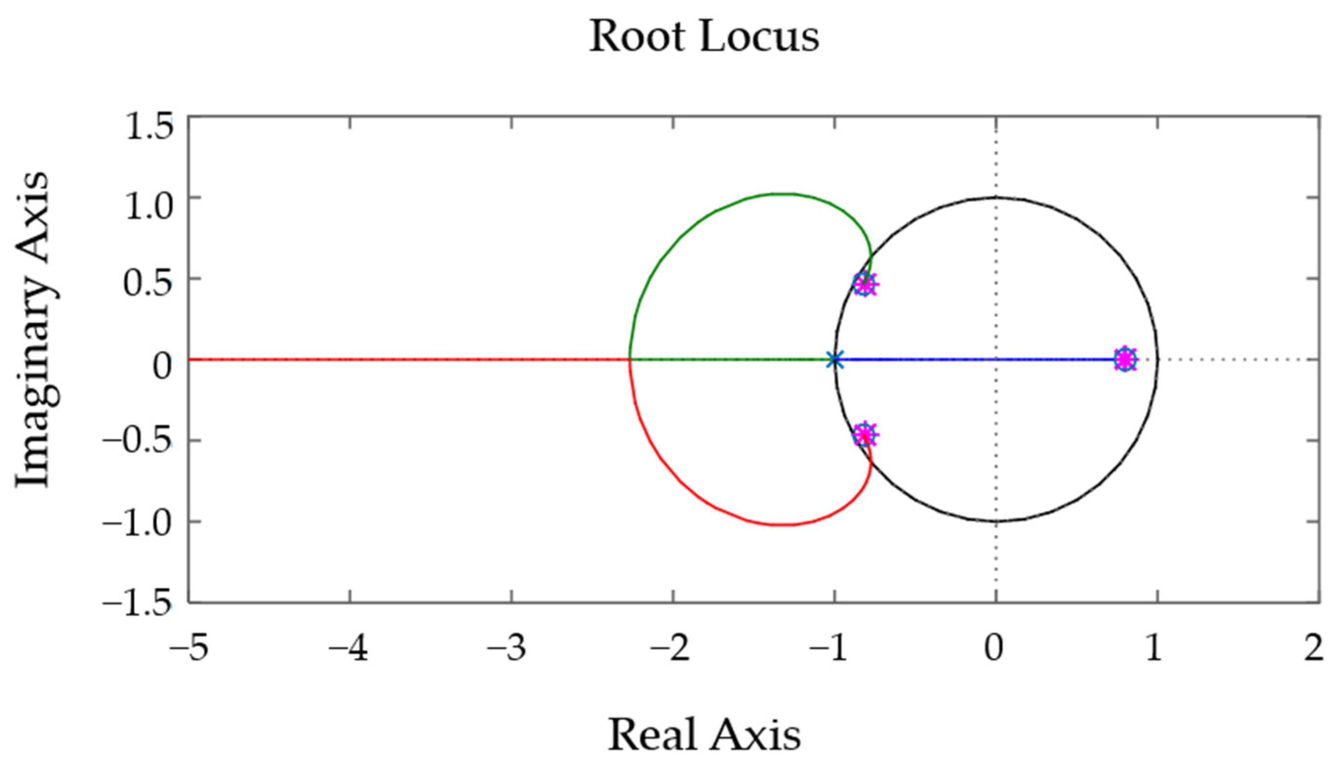
4. Stability Analysis of the Proposed Method

Previous research has shown that algorithm stability is crucial for tackling nonlinear systems. There are two stability analysis methods for numerical integration algorithms. The first method involves analyzing the value of the eigenvalue of the algorithm amplification matrix [44]. The second method involves searching for a transfer function that corresponds to the algorithm using discrete control theory and scrutinizing the poles derived from that function [16]. Chen and Ricle conducted a stability analysis of an algorithm utilizing discrete control theory [45]. The transfer function of the method was derived by applying the z-transform, and the consistency of the discrete transfer function that was produced consequently was evaluated by looking at the position of the poles on the z-plane. The positioning of the poles is a crucial factor in determining the stability of a system. One cannot consider a system to be stable until all of its poles are contained inside the unit circle. On the other hand, the system is regarded as unstable if a pole is found to be situated outside of the unit circle. According to reference [45], in this part, an investigation into the stability of the innovative algorithm is carried out using the theory as a foundation. The investigation focuses on systems that include nonlinear restoring forces and nonlinear damping forces. This study is carried out by making use of the root locus approach, which was previously reported in the body of scholarly work by Chen and Ricles.

4.1. Stability Analysis for Solving Systems with Nonlinear Restoring Force

Assuming the presence of a single-degree-of-freedom (SDoF) system characterized by a nonlinear restoring force and a linear damping force, it is possible to reformulate Equation (38) as follows:

$$\left(\frac{4}{\Delta t^2}m+\frac{2}{\Delta t}c+k_1\right)\Delta d_n=g_{n+1}+m{a}_n-f(d_n)+\left(c+\frac{4}{\Delta t}m\right)v_n,$$

(42)

where

$$k_1={\frac{\partial f(d)}{\partial d}|}_{d=d_n}.$$

(43)

In accordance with Equation (42), the equation for the preceding time step is:

$$\left(\frac{4}{\Delta t^2}m+\frac{2}{\Delta t}c+k_0\right)\Delta d_{n-1}=g_n+m{a}_{n-1}+\left(c+\frac{4}{\Delta t}m\right)v_{n-1}-f(d_{n-1}),$$

(44)

where

$$k_0={\frac{\partial f(d)}{\partial d}|}_{d=d_{n-1}}.$$

(45)

The relationship of the previous step can be expressed using Equations (39) and (40):

$$v_n=-v_{n-1}+\frac{2}{\Delta t}\Delta d_{n-1},$$

(46)

$$a_n=\frac{4}{\Delta t^2}\Delta d_{n-1}-\frac{4}{\Delta t}{v}_{n-1}-a_{n-1}.$$

(47)

Upon the substitution of Equations (39) and (40) into Equation (44), the following outcome is obtained:

$$a_n=\frac{4}{\Delta t^2}\Delta d_{n-1}-\frac{4}{\Delta t}{v}_{n-1}-a_{n-1}.$$

(48)

Comparing Equations (42) and (48) and considering Equation (36) yields

$$\left(\frac{4}{\Delta t^2}m+\frac{2}{\Delta t}c+k_1\right)\Delta d_n-k_0\Delta d_{n-1}=\Delta g_n+2m{a}_n+2c{v}_n+\frac{4m}{\Delta t}{v}_n-\left(f(d_n)-f(d_{n-1})\right).$$

(49)

When $\Delta t$ is small, it is possible to approximate the increment of restoring force as [46]:

$$\left(f(d_n)-f(d_{n-1})\right)=k_t\left(d_n-d_{n-1}\right),$$

(50)

where, $d_n-d_{n-1}$ can be computed by

$$d_n-d_{n-1}=\Delta d_{n-1}.$$

(51)

Substituting Equation (51) into Equation (50) yields

$$\left(f(d_n)-f(d_{n-1})\right)=k_t\Delta d_{n-1}.$$

(52)

Substituting Equation (52) into Equation (49) yields

$$\left(\frac{4}{\Delta t^2}m+\frac{2}{\Delta t}c+k_1\right)\Delta d_n-k_0\Delta d_{n-1}=\Delta g_n+2m{a}_n+2c{v}_n+\frac{4m}{\Delta t}{v}_n-k_t\Delta d_{n-1}.$$

(53)

Using the z-transformation to modify Equations (39)–(41), together with the delay theorem, we get the following result:

$$v_n(z)=\frac{2}{\Delta t}\frac{1}{(z+1)}\Delta d_n(z),$$

(54)

$$a_n(z)=\frac{4}{\Delta t^2}\frac{1}{z+1}\Delta d_n(z)-\frac{4}{\Delta t}\frac{1}{z+1}{v}_n(z),$$

(55)

$$\Delta d_{n-1}(z)=\frac{1}{z}\Delta d_n(z).$$

(56)

The equation represented as (52) is subjected to transformation by z-transformation. The resulting equation is then substituted with Equations (54)–(56) into the equation represented as (53).

$$\begin{array}{l}\left(\frac{4}{\Delta t^2}m+\frac{2}{\Delta t}c+k_1-\frac{k_0}{z}\right)\Delta d_n\left(z\right)\\ =\Delta g_n\left(z\right)+\left(\frac{16m}{\Delta t^2}\frac{1}{(z+1)}-\frac{16m}{\Delta t^2}\frac{1}{{(z+1)}^2}+\frac{4}{\Delta t}\frac{c}{(z+1)}-k_t\frac{1}{z}\right)\Delta d_n(z)\end{array}.$$

(57)

When Equation (57) is taken into consideration, the closed-loop block diagram of the proposed method can be seen in Figure 1. This diagram is applicable to systems that include a nonlinear restoring force.

The transfer functions for both the forward and feedback systems depicted in the block diagram in Figure 1 are presented as follows:

$$G^{\prime }={\left(\frac{4}{\Delta t^2}m+\frac{2}{\Delta t}c+k_1-\frac{k_0}{z}\right)}^{-1},$$

(58)

$$H=-\left(\frac{16m}{\Delta t^2}\frac{1}{(z+1)}-\frac{16m}{\Delta t^2}\frac{1}{{(z+1)}^2}+\frac{4}{\Delta t}\frac{c}{(z+1)}-k_t\frac{1}{z}\right).$$

(59)

The transfer function of the full closed-loop system is as follows:

$$G_{\mathrm{cl}}=\frac{G^{\prime }}{1+G^{\prime }H}=\frac{{(z+1)}^{2}z}{R(z)z^3+S(z)z^2+U(z)z+\left(k_t-k_0\right)}.$$

(60)

where

$$R(z)=\frac{4m}{\Delta t^2}+\frac{c}{2\Delta t}+k_1,S(z)=-\frac{8m}{\Delta t^2}-\frac{3c}{\Delta t}+2k_1-k_0+k_t,U(z)=\frac{4m}{\Delta t^2}-\frac{7}{2\Delta t}c+k_1-2k_0+2k_t.$$

It is possible to obtain the characteristic equation of the transfer function as follows:

$$R(z)z^3+S(z)z^2+U(z)z+\left(k_t-k_0\right)=0,$$

(61)

Equation (61) can be expressed in the root locus form:

$$1+k_t\frac{{\left(z+1\right)}^2}{R(z)z^3+\left(-\frac{8m}{\Delta t^2}-\frac{3c}{\Delta t}+2k_1-k_0\right)z^2+\left(\frac{4m}{\Delta t^2}-\frac{7}{2\Delta t}c+k_1-2k_0\right)z-k_0}=0,$$

(62)

The root locus is plotted in MATLAB using Equation (62). In this section, the arithmetic example in reference [46], the SDoF system with structural parameters of $m=1\mathrm{kg}$, $k_0=5{\pi }^2\mathrm{N}/\mathrm{m}$, $k_1=4{\pi }^2\mathrm{N}/\mathrm{m}$, $c=0$, and $\Delta t=0.5\mathrm{s}$ is researched. The root locus with a variable parameter of k_t can be expressed as:

$$1+k_t\frac{z^2+2z+1}{\left(16+4{\pi }^2\right)z^3-(32-3{\pi }^2)z^2+(16-6{\pi }^2)z-5{\pi }^2}=0,$$

(63)

Figure 2 displays the obtained root locus diagram.

The unit circle is depicted by the black line, as illustrated in Figure 2. The stability of this algorithm is observed in the unit circle. The algorithm exhibits instability beyond the unit circle. Every point within the k_t domain is situated within the boundaries of the unit circle. Empirical evidence suggests that this approach exhibits unconditional stability when applied to nonlinear structures.

4.2. Stability Analysis for Solving Systems with Nonlinear Restoring Force

Assuming an SDoF system with a linear restoring force and a nonlinear damping force, it is possible to reformulate Equation (39) as follows:

$$\left(\frac{4}{\Delta t^2}m+\frac{2}{\Delta t}{c}_1+k\right)\Delta d_n=g_{n+1}+m\frac{4}{\Delta t}{v}_n+m{a}_n-h\left(-v_n\right)-k{d}_n,$$

(64)

where

$$c_1={\frac{\partial h(v)}{\partial v}|}_{v=-v_n}.$$

(65)

The preceding integral step solution is given by Equation (65):

$$\left(\frac{4}{\Delta t^2}m+\frac{2}{\Delta t}{c}_0+k\right)\Delta d_{n-1}=g_n+m\frac{4}{\Delta t}{v}_{n-1}+m{a}_{n-1}-h\left(-v_{n-1}\right)-k{d}_{n-1},$$

(66)

where

$$c_0={\frac{\partial h(v)}{\partial v}|}_{v=v_{n-1}}.$$

(67)

Taking Equations (39) through (41) into consideration, the preceding integration step has a corresponding relationship:

$$c_0={\frac{\partial h(v)}{\partial v}|}_{v=v_{n-1}}\frac{2}{\Delta t}{c}_0\Delta d_{n-1}+k\Delta d_{n-1}=g_n-h\left(-v_{n-1}\right)-k{d}_{n-1}-m{a}_n.$$

(68)

When Equations (64) and (68) are compared, together with Equation (36), the result is that:

$$\begin{array}{l}\left(\frac{4}{\Delta t^2}m+\frac{2}{\Delta t}{c}_1+k\right)\Delta d_n-\left(\frac{2}{\Delta t}{c}_0+k\right)\Delta d_{n-1}\\ =\Delta g_n+2m{a}_n+2c_t{v}_n-\frac{2}{\Delta t}{c}_t\Delta d_{n-1}-k{d}_n+k{d}_{n-1}+\frac{4m{v}_n}{\Delta t}\end{array},$$

(69)

where

$$c_t=\frac{h\left(-v_n\right)-h\left(-v_{n-1}\right)}{\left(-v_n\right)-\left(-v_{n-1}\right)}.$$

(70)

By applying the z-transform to Equation (69) and subsequently incorporating Equations (54)–(56) into the transformed equation, we can obtain the desired result:

$$\begin{array}{l}\left(\frac{4}{\Delta t^2}m+\frac{2}{\Delta t}{c}_1+k-\frac{2}{\Delta tz}{c}_0-\frac{k}{z}\right)\Delta d_n(z)\\ =\Delta g_n(z)+\left(\frac{8m}{\Delta t^2(z+1)}+\frac{4c_t}{\Delta t(z+1)}-\frac{2}{\Delta tz}{c}_t-k\frac{1}{z}\right)\Delta d_n(z)\end{array}.$$

(71)

When Equation (71) is taken into consideration, the closed-loop block diagram of the proposed method is as shown in Figure 2, and it applies to systems with nonlinear restoring force.

The forward transfer functions and feedback transfer functions shown in the block diagram in Figure 1 may each have an equation that can be represented as:

$$G^{\prime }={\left(\frac{4}{\Delta t^2}m+\frac{2}{\Delta t}{c}_1+k-\frac{2}{\Delta tz}{c}_0-\frac{k}{z}\right)}^{-1},$$

(72)

$$H=-\left(\frac{8m}{\Delta t^2(z+1)}+\frac{4c_t}{\Delta t(z+1)}-\frac{2}{\Delta tz}{c}_t-k\frac{1}{z}\right).$$

(73)

The transfer mechanism for the complete closed-loop system has been provided with:

$$\begin{array}{ll}{G}_{\mathrm{cl}}& =\frac{G^{\prime }}{1+G^{\prime }H}\\ & =\frac{(z+1)z}{\left(\frac{4m}{\Delta t^2}+\frac{2c_1}{\Delta t}+k\right)z^2+\left(-\frac{4m}{\Delta t^2}+\frac{2c_1}{\Delta t}+k-\frac{2c_0}{\Delta t}-\frac{2c_t}{\Delta t}\right)z+\left(\frac{2c_t}{\Delta t}-\frac{2c_0}{\Delta t}\right)}\end{array}.$$

(74)

The derivation of the characteristic equation for the transfer function can be achieved by means of a specific mathematical procedure:

$$\left(\frac{4m}{\Delta t^2}+\frac{2c_1}{\Delta t}+k\right)z^2+\left(-\frac{4m}{\Delta t^2}+\frac{2c_1}{\Delta t}+k-\frac{2c_0}{\Delta t}-\frac{2c_t}{\Delta t}\right)z+\left(\frac{2c_t}{\Delta t}-\frac{2c_0}{\Delta t}\right)=0.$$

(75)

The equation denoted as Equation (75) is presented in the format of the root locus.

$$1+c_t\frac{\frac{2}{\Delta t}\left(1-z\right)}{\left(\frac{4m}{\Delta t^2}+\frac{2c_1}{\Delta t}+k\right)z^2+\left(-\frac{4m}{\Delta t^2}+\frac{2c_1}{\Delta t}+k-\frac{2c_0}{\Delta t}\right)z-\frac{2c_0}{\Delta t}}=0.$$

(76)

The root locus expression is derived through the substitution of the structural variables, specifically the values of $m=1\mathrm{kg}$, $k=4{\pi }^2\mathrm{N}/\mathrm{m}$, $c_0=3.5\mathrm{N}\cdot \mathrm{s}/\mathrm{m}$, $c_1=2.5\mathrm{N}\cdot \mathrm{s}/\mathrm{m}$, and $\Delta t=0.5\mathrm{s}$. Figure 3 displays the root locus diagram.

$$1+c_t\frac{4-4\mathrm{z}}{\left(26+4{\pi }^2\right)z^2+\left(4{\pi }^2-20\right)z-14}=0.$$

(77)

The fact that all of the points of c_t in Figure 3 are contained inside the unit circle demonstrates that the suggested approach is unquestionably stable in nonlinear systems of this kind.

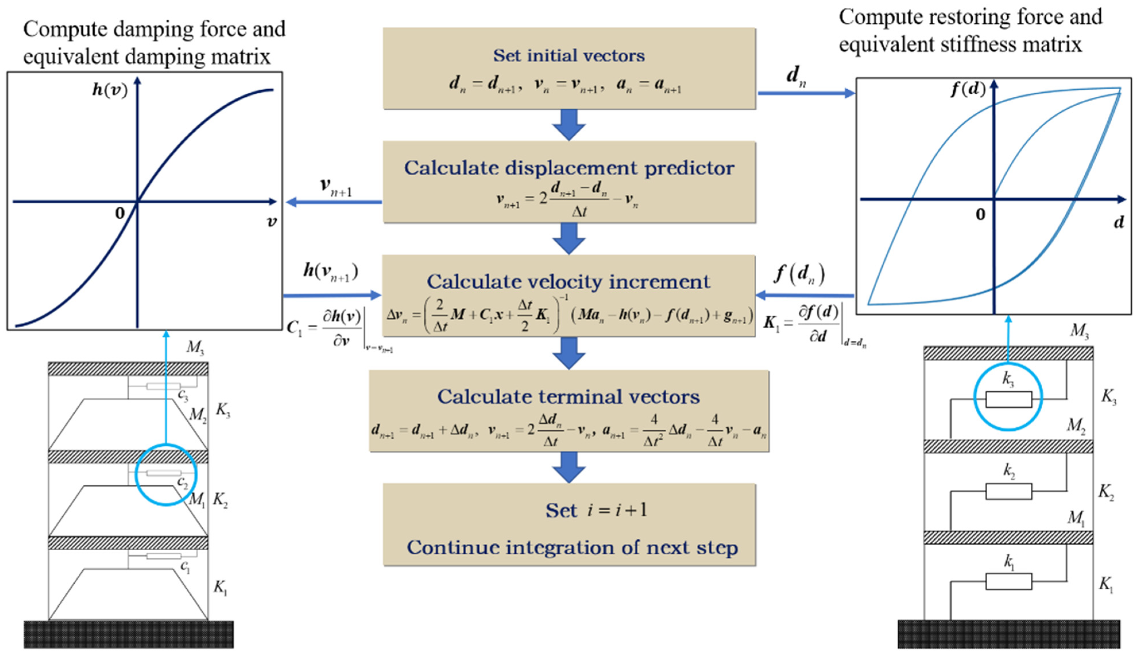
4.3. Calculation Process of the Proposed Method

The integration process of the proposed method, as shown in Figure 4, is as follows:

Step 1. Determine the starting vectors, which are denoted by $d_n$, $v_n$, and $a_n$. The nonlinear damping model should have $d_n$ included where appropriate. Perform the calculations necessary to determine the damping force and equivalent stiffness matrix.

Step 2. Figure out the displacement predictor $v_{n+1}$. In the nonlinear restoring force model, substitute $v_{n+1}$ for the previous value. Determine the restoring force, and then compute the comparable damping matrix.

Step 3. Create the nonlinear vectors $h\left(v_{n+1}\right)$ and $f\left(d_{n+1}\right)$, as well as the $C_1$ and $K_1$ matrices that are comparable to them. Determine the increase in velocity by using Equation (33).

Step 4. Using Equations (33) and (34), determine the values of the terminal vectors $d_{n+1}$, $v_{n+1}$, and $a_{n+1}$.

Step 5. Proceed with the integration of the subsequent time step.

5. Analysis of the Applicability and Reliability of the Proposed Method

The preceding section elucidates a comprehensive process of deriving the technique and establishes its stability in numerical computations through theoretical analysis. In this part, we will evaluate the effectiveness of the suggested technique in terms of its computing performance when applied to the solution of nonlinear issues.

5.1. Accuracy Analysis of the Proposed Method

The temporal resolution is a crucial parameter that impacts both the precision and effectiveness of the computational integration methodology [43]. For the purpose of accuracy analysis, a Bouc–Wen model from a previously published work [47] has been chosen. The non-linear restoring force model mentioned above is subjected to sinusoidal excitation, and the discrepancies in the outcomes obtained with varying step sizes are evaluated.

In this part, the shear structural model that is chosen is a three-layer model, and Figure 5 displays the pattern of this model. The parameters of the model are as follows: the mass of the 1st story is 2.3 × 10⁴ kg, the mass of the 2nd story is 1.6 × 10⁴ kg, and the mass of the 3rd story is 1.4 × 10⁴ kg; the stiffness of the 1st story is 1.5 × 10⁷ N/m, the stiffness of the 2nd and 3rd story is 2 × 10⁷ N/m. Within the framework of the model, a Rayleigh damping that has a structure-based damping ratio of 5% is considered. Soft steel dampers may be found on each level of the building. The findings were derived from the published work [48] and were obtained by value fitting of quasi-static test and shaking table experiment information with governed displacement. The Bouc–Wen model of variables was used to pick these values, which were as follows: $k_0=3.70\mathrm{kN}/\mathrm{mm}$, $n=1$, $\gamma =-1000$, and $\beta =652.7$. The length of the sinusoidal wave is five seconds, the maximum acceleration is 0.2 g, the period of the wave is two cycles per second, and both the starting displacement and initial velocity are zero. Matlab is used to perform the analysis on the simulations once they have been run. The first proposed technique for calculating the average acceleration a time interval of Δt = 0.00001 s is used as the benchmark solution.

When calculating the top displacement of the model, we employed the approach that was presented, as well as Chang’s method and the CR method. The findings are summarized in

Table 1. Errors under different time steps.

Time Steps	New Algorithm	CR Method	Chang Method
$\Delta t$ = 0.01	−7.43 × 10−8	−9.46 × 10−7	−9.51 × 10−7
$\Delta t$ = 0.001	−7.50 × 10−10	−1.09 × 10−8	−1.10 × 10−8
$\Delta t$ = 0.0001	−7.51 × 10−12	−1.28 × 10−10	−1.28 × 10−10

, where it can be shown that there is a high level of concordance between the findings for the time increments of 0.001 s, 0.0001 s, and 0.01 s. Table 1 displays, at a time step of 0.05 s, the errors that result from using various numerical integration techniques for different time steps.

According to Table 1, it can be observed that the proposed method exhibits a comparatively lower calculation error in comparison to the Chang and CR methods. This suggests that, under the given conditions, the proposed method is more precise. Furthermore, the suggested approach exhibits second-order accuracy and remains consistent with the initial mean acceleration computation technique.

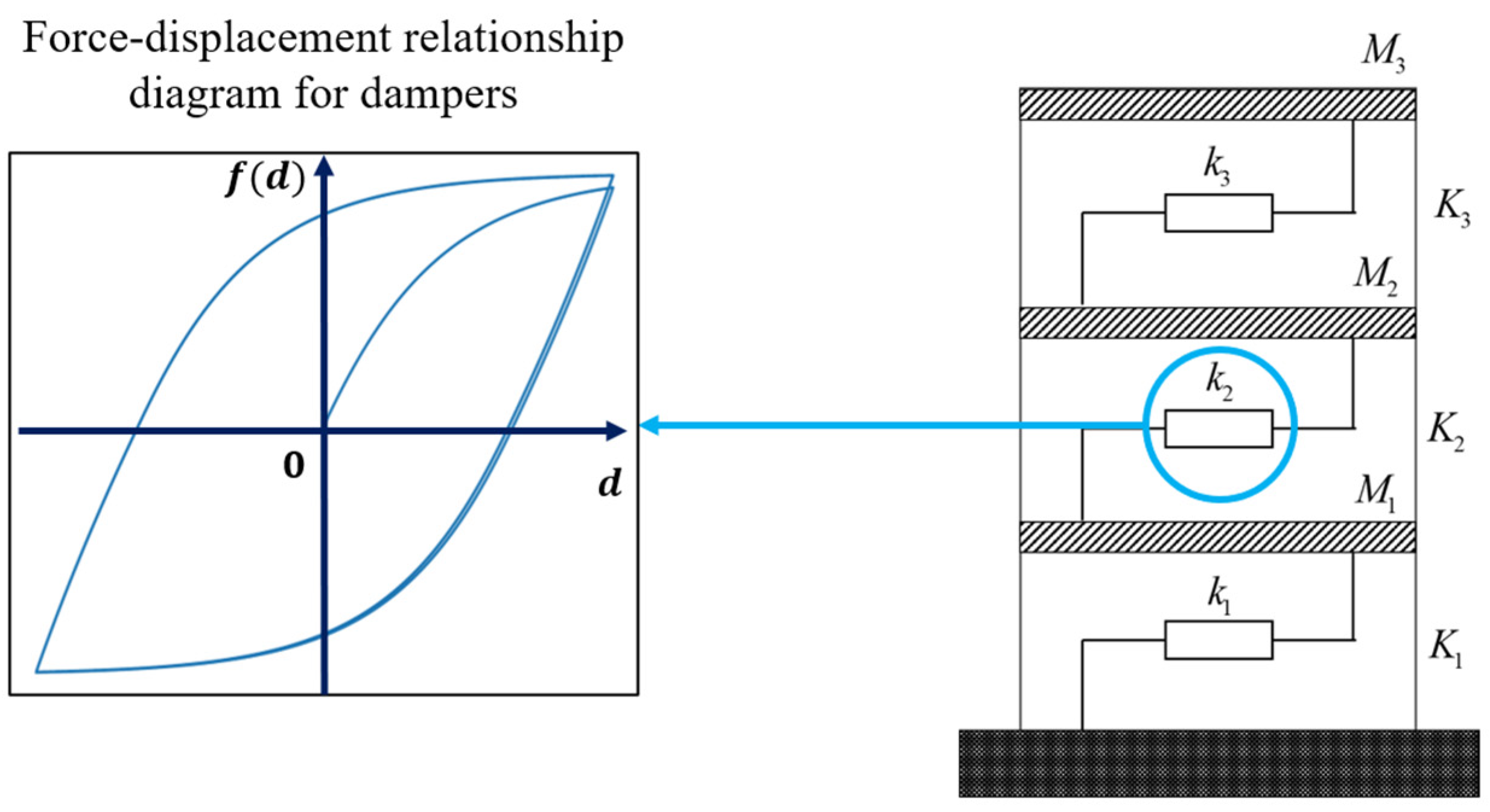
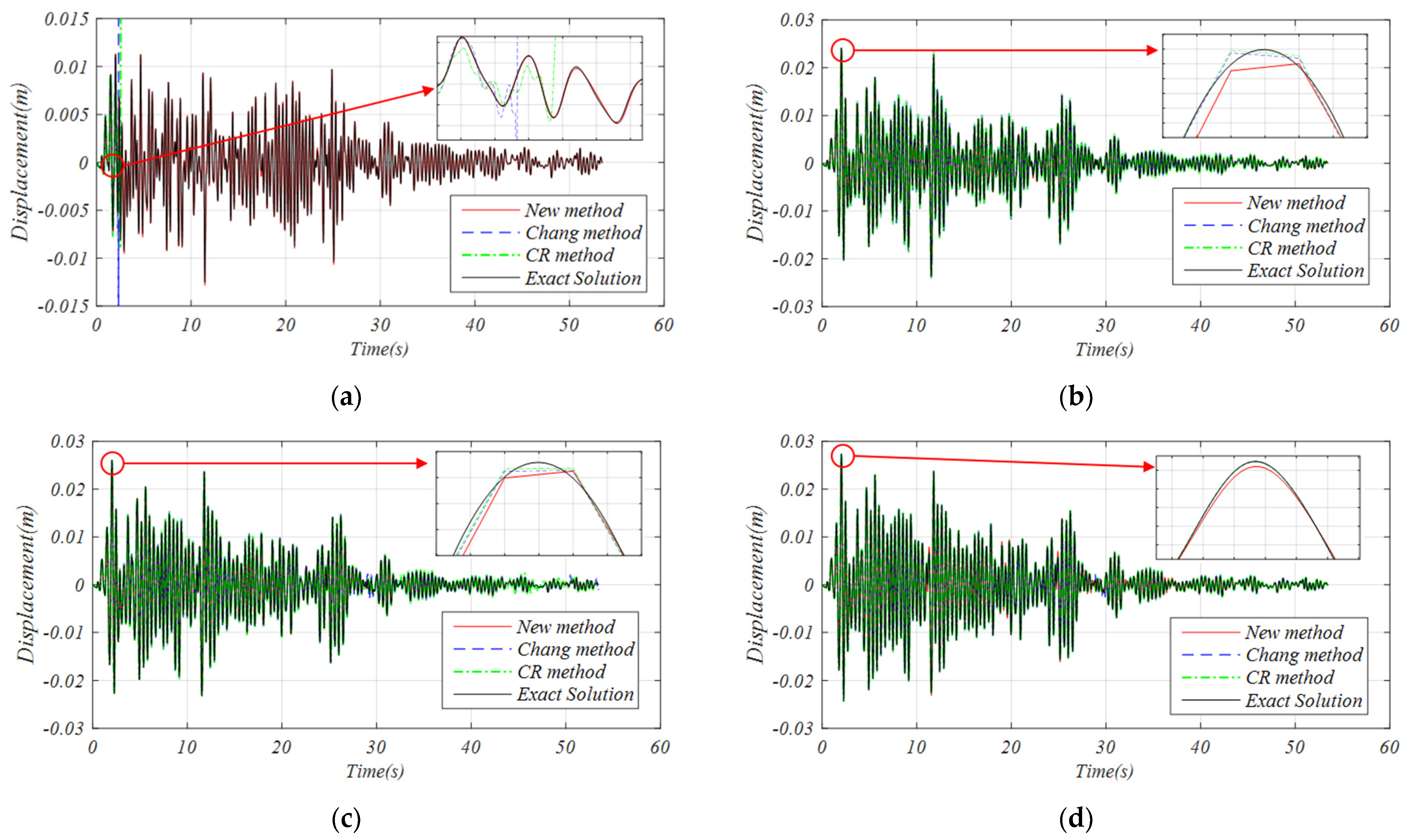
5.2. Numerical Simulation of a Nonlinear Restoring Force Structure

The validation model employed in this particular subsection is equivalent in quality to the one utilized in the preceding subsection. The definition of four distinct scenarios is as follows: the value of $\gamma$ in Scenario I is −1000, the value of $\gamma$ in Scenario II is −200, the value of $\gamma$ in Scenario III is 200, and the value of $\gamma$ in Scenario IV is 1000; the value of $\beta$ in each scenario is 652.7. Each scenario is characterized by a unique value of $k_0=3.70\mathrm{kN}/\mathrm{mm}$, n = 1, and varying values of γ and β. The El-Centro wave, which has a peak acceleration of 0.2 g, is employed as the external excitation.

The time step that is used in the calculation of the reference solution in the recommended technique, the Chang method, and the CR method is set to $\Delta t=0.001\mathrm{s}$, while the time step that is used in the calculation of the reference solution in the original mean acceleration method is $\Delta t=0.0001\mathrm{s}$. The seismic response curves of the top displacement are shown in Figure 6. These seismic response curves were calculated using the recommended methodology, the Chang method, the CR method, and the corresponding reference solution, in that order.

Table 2. The relative error of the displacement maximum relative to the reference solution.

γ	New Algorithm	CR Method	Chang Method
−1000	0.20%	destabilization	destabilization
−200	0.20%	0.01%	0.05%
200	0.13%	0.09%	0.12%
1000	0.10%	0.08%	0.03%

displays the relative errors that were found between the reference solution and the maximum displacement phase.

As shown in Figure 6, the results of the nonlinear example of calculation are given. It is noted that the errors between the displacement curves of the proposed method and the reference solution are relatively small. As can be shown in Figure 6a, in contrast to the Chang and CR approaches, the suggested method’s core stays constant throughout the length of the seismic wave. Table 2 shows that the suggested technique has high stability and favorable accuracy in such non-linear systems, as demonstrated by the relative errors.

5.3. Numerical Simulation of a Nonlinear Restoring Force Structure

As shown in Figure 7, the current part makes use of a structural model consisting of three layers with nonlinear viscous dampers placed on each level. The exact parameters of the structural model are as follows: the mass of the 1st story is 8 × 10⁵ kg, the mass of the 2nd and 3rd stories is 10 × 10⁵ kg; the stiffness of the 1st, 2nd, and 3rd story is 3 × 10⁶ N/m. Both the features of the seismic wave and the damping of the structure have been preserved in the same manner in which they were found before. In order to accurately characterize the viscous damper present on each level, the Kelvin–Voigt model is used. The corresponding calculation formula for this model is

$$F(t)=k_{d}d+sign\left(v(t)\right)c{\left|v(t)\right|}^{\alpha }.$$

(78)

where the stiffness coefficient is given as $k_d=$ 0, the value of the damping coefficient is given as $c=\mathrm{46,000}\mathrm{N}\cdot \mathrm{s/m}$, and various degrees of nonlinearity are taken into consideration ($\alpha =0.1$, $\alpha =0.3$, $\alpha =0.5$, and $\alpha =0.7$, correspondingly for the nonlinear degrees).

The time step that is supposed to be used for the suggested method, Chang method, and CR method is $\Delta t=0.001\mathrm{s}$, but the time step that is used for the reference solution in the traditional average acceleration methodology is $\Delta t=0.0001\mathrm{s}$. The time step is the same in all three methods: the recommended approach, the Chang method, and the CR method. Figure 8 depicts the time history curves of the top story displacement, which were estimated using the suggested technique, the Chang method, the CR method, and the original average acceleration method. These methods were used to determine the displacement.

Table 3. The relative error of the displacement maximum relative to the reference solution.

A	New Algorithm	CR Method	Chang Method
0.1	0.03%	0.01%	2.19%
0.3	0.06%	0.04%	2.22%
0.5	0.08%	0.07%	2.25%
0.7	0.07%	0.09%	2.27%

illustrates the relative errors that are associated with the maximum displacement phase and the reference solution.

Figure 8 indicates that the proposed method remains stable, and the displacement curve is in good agreement with the reference solution.

When the relative errors shown in Figure 8a through Figure 8d and Table 3 are compared, it is possible to see that the solutions produced via the proposed technique have higher closeness to the solution used as a reference in comparison to the solutions obtained using the Chang approach. The proposed technique and the CR method both have favorable accuracy. This can be seen when the two sets of data are compared to one another. This trend is particularly pronounced in cases of heightened nonlinearity. When applied to structures that have a large amount of damping nonlinearity, the approach that has been provided demonstrates a satisfactory level of application and dependability. As a result of this, the method can be recommended.

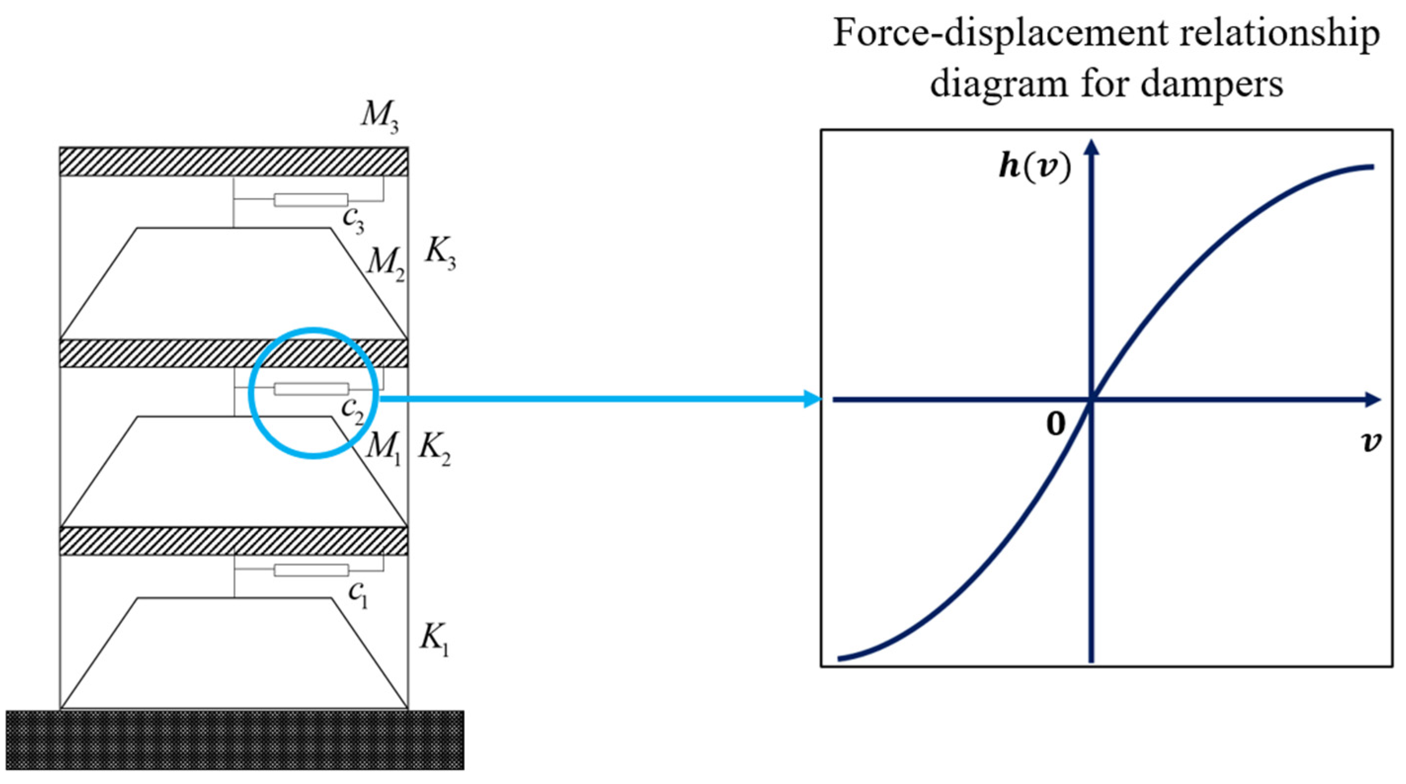
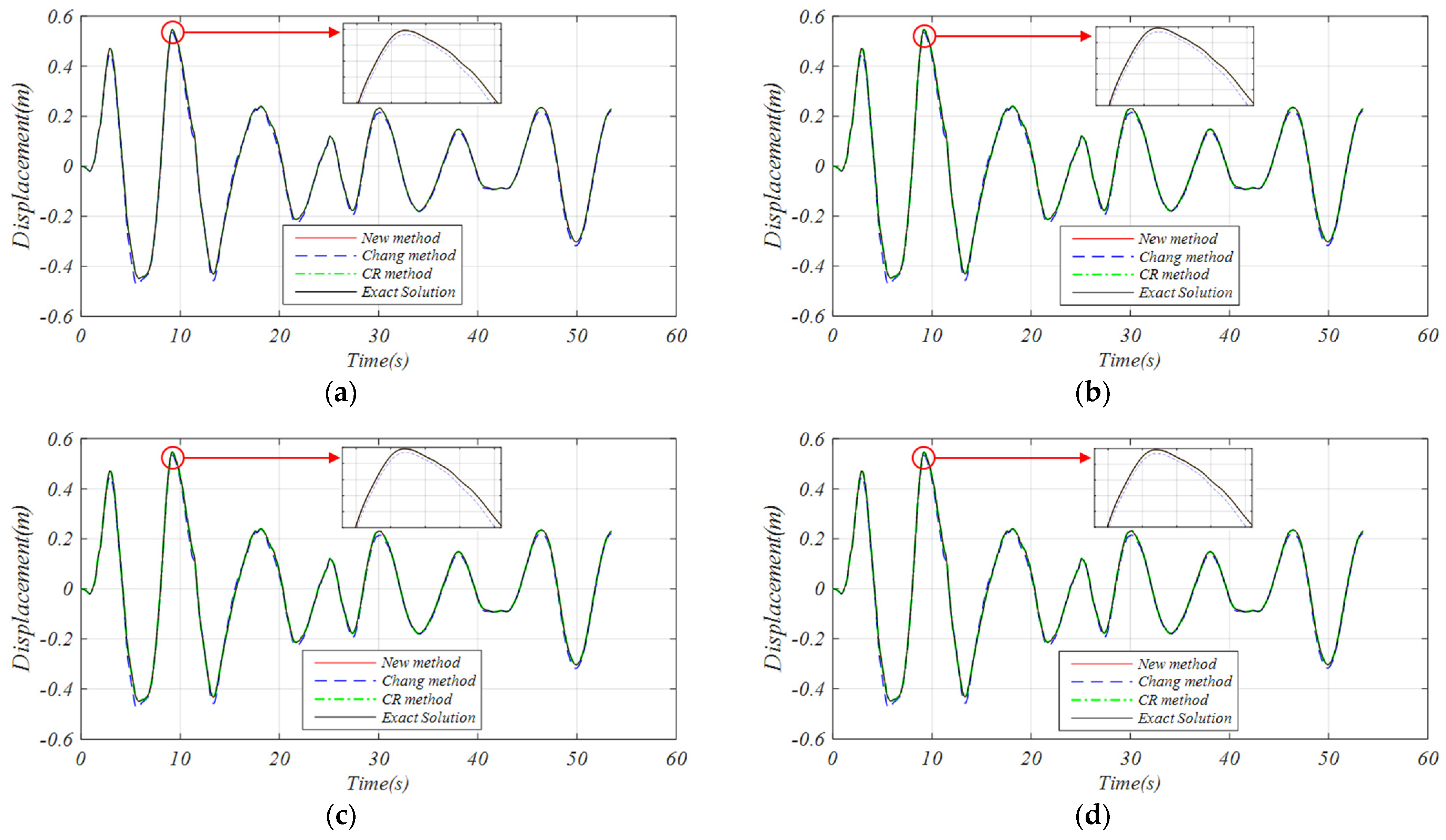
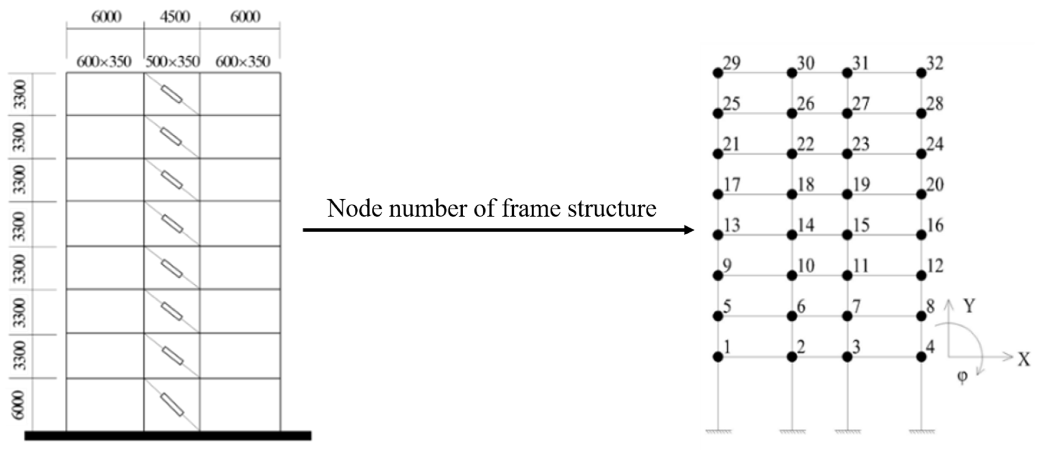
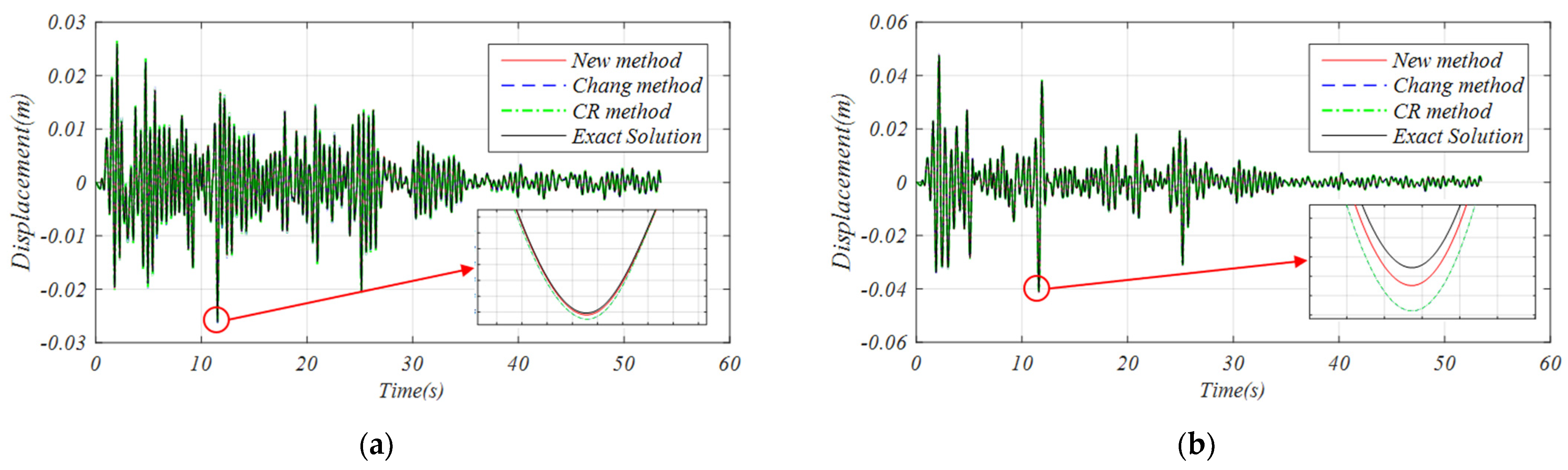
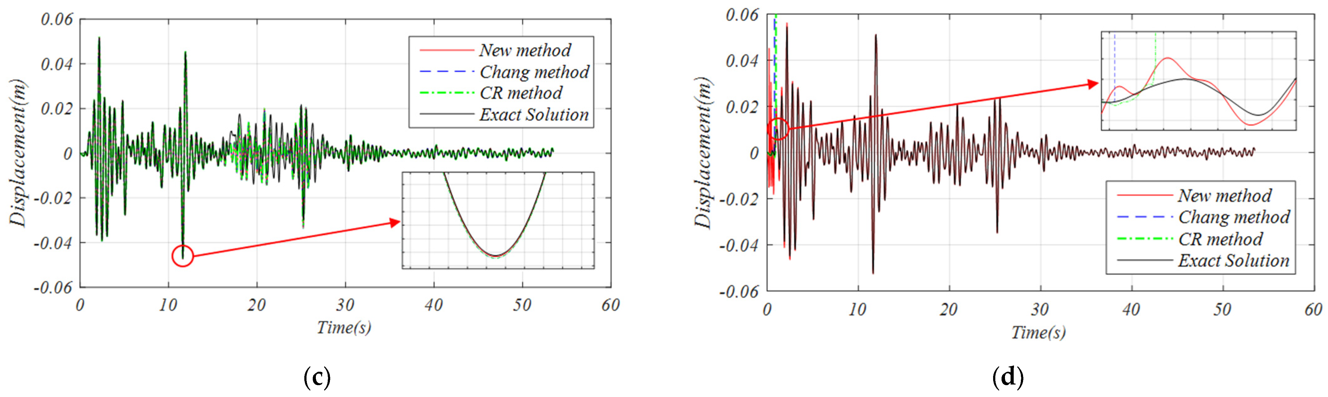
5.4. Numerical Simulation of an MDoF Frame Structure

In order to conduct a thorough evaluation of the efficacy of the suggested approach in addressing seismic response in MDoF structures, a structural model with multiple degrees of freedom was developed based on the framework presented in a prior publication [49]. The structure in question is a concrete frame building consisting of eight stories and three spans. While Figure 9 is a depiction of the model’s schematic design. The specifics of the beams and columns that make up the structure are as follows: the columns are 600 × 600, the edge beams are 600 × 350, and the intermediate beams are 500 × 350. The structure under discussion comprises a total of 96 degrees of freedom, with each node showing two translational degrees of freedom in the x and y axes as well as one rotating degree of freedom. This gives each node a total of 96 degrees of freedom. On each level, a damper made of soft steel has been placed. In this investigation, the Bouc–Wen model is used in order to illustrate the relationship that exists between the dampers’ displacement and the force that they exert. The seismic wave that is being considered in this context is the same as the one that was considered above.

The simulation was conducted while considering four distinct scenarios that exhibit varying degrees of hysteresis performance in terms of restoring force, as illustrated in Section 5.1. The temporal resolution for the Chang method, CR method, and the proposed method is $\Delta t=0.001\mathrm{s}$, while the corresponding solution is obtained using the original normal acceleration method with a finer temporal resolution of $\Delta t=0.0001\mathrm{s}$. Figure 10 illustrates the suggested technique, together with the Chang method, the CR method, and the reference solution’s respective findings on the x-directional displacement response curves of node 32. The relative inaccuracy that pertains to the minimal displacement value in comparison to the solution used as a reference is shown in

Table 4. The relative error of the displacement maximum relative to the reference solution.

γ	New Algorithm	CR Method	Chang Method
−1000	0.74%	2.52%	2.48%
−200	0.15%	0.92%	0.93%
200	0.07%	0.51%	0.52%
1000	3.22%	destabilization	destabilization

.

According to the relative errors shown in Figure 10 and Table 4, the reference solution and the displacement curves correspond to one another quite well, and the differences are contained within a somewhat narrow margin. In addition, the recommended approach is secure in each and every one of the many scenarios, while the conventional Chang method and the CR method both display volatile instability, as shown in Figure 10c. This demonstrates that the novel approach is applicable to nonlinear MDoF frame structures in a useful way.

6. Conclusions

This paper presents a novel approach that introduces a linearly implicit algorithm featuring an explicit displacement expression, which draws inspiration from the Rosenbrock method’s strategy. The technique that is being considered integrates one Newton iteration into the mean acceleration method. The displacement term is used in lieu of the iteration variable in order to carry out the built-in Newton iteration that is a part of the method. In this paper, the root locus is used to perform an analysis of the stability of a technique that has been suggested for the modeling of systems that include both nonlinear restoring force and nonlinear damping force. The following is a concise summary of the findings and conclusions:

(1)

The proposed method utilizes a double explicit format and may be used for the solution of nonlinear problems involving restoring force as well as nonlinear issues involving damping force.

(2)

The approach that has been suggested is unconditionally stable in nonlinear damping force problems in addition to nonlinear restoring force problems.

(3)

Compared with the Chang and CR approaches, the accuracy of the nonlinear restoring force structure obtained by the suggested method is rather high, leading to its advantages in application and dependability in nonlinear systems.

The unconditionally stable linear implicit integration algorithm proposed in this paper can be effectively applied to the structural dynamic equations with nonlinearity, which is beneficial to solving nonlinear dynamic problems in engineering practice.

In the future, along the lines of the tactics outlined in this paper, additional implicit methods might be used to produce linearly implicit methods that are more accurate. This would apply to nonlinear situations.

References

1. Hu, R.; Hu, S.; Yang, M.; Zhang, Y. Metallic Yielding Dampers and Fluid Viscous Dampers for Vibration Control in Civil Engineering: A Review. Int. J. Struct. Stab. Dyn. 2022, 22, 2230006. [Google Scholar] [CrossRef]
2. Imaduddin, F.; Mazlan, S.A.; Zamzuri, H. A design and modelling review of rotary magnetorheological damper. Mater. Design 2013, 51, 575–591. [Google Scholar] [CrossRef]
3. Yang, F.; Sedaghati, R.; Esmailzadeh, E. Vibration suppression of structures using tuned mass damper technology: A state-of-the-art review. J. Vib. Control 2022, 28, 812–836. [Google Scholar] [CrossRef]
4. Li, S.; Chen, Y.T.; Chai, Y.H.; Li, B. Effects of brace stiffness and nonlinearity of viscous dampers on seismic performance of structures. Int. J. Struct. Stab. Dyn. 2021, 21, 2150188. [Google Scholar] [CrossRef]
5. Dall, A.; Tubaldi, E.; Ragni, L. Influence of the nonlinear behavior of viscous dampers on the seismic demand hazard of building frames. Earthq. Eng. Struct. Dyn. 2016, 45, 149–169. [Google Scholar]
6. Du, X.Q.; Yang, D.X.; Zhou, J.L.; Yan, X.L.; Zhao, Y.L.; Li, S. New Explicit Integration Algorithms with controllable numerical dissipation for structural dynamics. Int. J. Struct. Stab. Dyn. 2018, 18, 1850044. [Google Scholar] [CrossRef]
7. Li, S.; Qin, L.B.; Guo, H.C.; Yang, D.X. A method of improving time integration algorithm accuracy for long-term dynamic simulation. Int. J. Struct. Stab. Dyn. 2020, 20, 2050079. [Google Scholar] [CrossRef]
8. Newmark, N.M. A method of computation for structural dynamics. J. Eng. Mech. Div. ASCE 1959, 85, 67–94. [Google Scholar] [CrossRef]
9. Wilson, E.L.; Farhoomand, I.; Bathe, K.J. Nonlinear dynamic analysis of complex structures. Earthq. Eng. Struct. Dyn. 1972, 1, 241–252. [Google Scholar] [CrossRef]
10. Park, K. An improved stiffly stable method for direct integration of nonlinear structural dynamic equations. J. Appl. Mech. 1975, 42, 464–470. [Google Scholar] [CrossRef]
11. Hilber, H.M.; Hughes, T.J.R.; Taylor, R.L. Improved numerical dissipation for time integration algorithms in structural dynamics. Earthq. Eng. Struct. Dyn. 1977, 5, 283–292. [Google Scholar] [CrossRef] [Green Version]
12. Wood, W.L.; Bossak, M.; Zienkiwicz, O.C. An alpha modification of Newmark’s method. Int. J. Numer. Methods Eng. 1980, 15, 1562–1566. [Google Scholar] [CrossRef]
13. Shao, H.; Cai, C. A three parameters algorithm for numerical integration of structural dynamic equations. Chin. J. Appl. Mech. 1988, 5, 76–81. [Google Scholar]
14. Chung, J.; Hulbert, G.M. A time integration algorithm for structural dynamics with improved numerical dissipation: The generalized-α method. J. Appl. Mech. ASME 1993, 60, 371–375. [Google Scholar] [CrossRef]
15. Bathe, K.J.; Baig, M.M.I. On a composite implicit time integration procedure for nonlinear dynamics. Comput. Struct. 2005, 83, 2513–2524. [Google Scholar] [CrossRef]
16. Wu, B.; Xu, G.; Wang, Q.; Williams, M. Operator-splitting method for real-time substructure testing. Earthq. Eng. Struct. Dyn. 2006, 35, 293–314. [Google Scholar] [CrossRef]
17. Rezaiee-Pajand, M.; Alamatian, J. Implicit higher-order accuracy method for numerical integration in dynamic analysis. J. Struct. Eng. 2008, 134, 973–985. [Google Scholar] [CrossRef]
18. Pajand, M.R.; Sarafrazi, S.R.; Hashemian, M. Improving stability domains of the implicit higher order accuracy method. Int. J. Numer. Meth. Eng. 2011, 88, 880–896. [Google Scholar] [CrossRef]
19. Shojaee, S.; Rostami, S.; Abbasi, A. An unconditionally stable implicit time integration algorithm: Modified quartic B-spline method. Comput. Struct. 2015, 153, 98–111. [Google Scholar] [CrossRef]
20. Gardner, D.J.; Woodward, C.S.; Reynolds, D.R. Implicit integration methods for dislocation dynamics. Model. Simul. Mat. Sci. Eng. 2015, 23, 025006. [Google Scholar] [CrossRef]
21. Shimada, M.; Hoitink, A.; Tamma, K.K. The fundamentals underlying the computations of acceleration for general dynamic applications: Issues and noteworthy perspectives. CMES Comput. Model. Eng. Sci. 2015, 104, 133–158. [Google Scholar]
22. Shimada, M.; Masuri, S.; Tamma, K.K. A novel design of an isochronous integration [iIntegration] framework for first/second order multidisciplinary transient systems. Int. J. Numer. Methods Eng. 2015, 102, 867–891. [Google Scholar] [CrossRef]
23. Hughes, T.J.R. The Finite Element Method; Prentice Hall: New Jersey, NJ, USA, 2001. [Google Scholar]
24. Bursi, O.S.; He, L.; Lamarche, C.; Bonelli, A. Linearly implicit time integration methods for real-time dynamic substructure testing. J. Eng. Mech. 2010, 136, 1380–1389. [Google Scholar] [CrossRef]
25. Zienkiewicz, O.C. The Finite Element Method; McGraw-Hill: New York, NY, USA, 1977. [Google Scholar]
26. Belytschko, T.; Hughes, T.J.R. Computational Methods for Transient Analysis; Elsevier: Amsterdam, The Netherlands, 1983. [Google Scholar]
27. Hughes, T.J.R. The Finite Element Method; Prentice-Hall: Englewood Cliffs, NJ, USA, 1987. [Google Scholar]
28. Yin, S.H. A new explicit time integration method for structural dynamics. Int. J. Struct. Stability. Dyn. 2013, 13, 1250068. [Google Scholar] [CrossRef]
29. Chen, C.; Ricles, J.M. Stability analysis of direct integration algorithms applied to MDOF nonlinear structural dynamics. J. Eng. Mech. 2008, 136, 485–495. [Google Scholar] [CrossRef]
30. Arnold, M.; Burgermeister, B.; Eichberger, A. Linearly implicit time integration methods in real-time applications DAEs and stiff ODEs. Multibody Syst. Dyn. 2007, 17, 99–117. [Google Scholar] [CrossRef]
31. Chi, F.D.; Wang, J.T.; Jin, F. Delay-dependent stability and added damping of SDOF real-time dynamic hybrid testing. Earth. Eng. Eng. Vib. 2010, 9, 425–438. [Google Scholar] [CrossRef]
32. Chang, S.Y. An explicit structure-dependent algorithm for pseudo dynamic testing. Eng. Struct. 2013, 46, 511–525. [Google Scholar] [CrossRef]
33. Chang, S.Y. Explicit pseudo dynamic algorithm with unconditional stability. J. Eng. Mech. ASCE 2002, 128, 935–947. [Google Scholar] [CrossRef]
34. Kolay, C.; Ricles, J.M. Assessment of explicit and semi-explicit classes of model-based algorithms for direct integration in structural dynamics. Int. J. Numer. Methods Eng. 2016, 107, 49–73. [Google Scholar] [CrossRef]
35. Li, S.; Yang, D.X.; Guo, H.C.; Liang, G. General formulation of eliminating unusual amplitude grow for structure-dependent integration algorithms. Int. J. Struct. Stab. Dyn. 2019, 20, 2050006. [Google Scholar] [CrossRef]
36. Chen, C.; Ricles, J.M. Development of direct integration algorithms for structural dynamics using discrete control theory. J. Eng. Mech. ASCE 2008, 134, 676–683. [Google Scholar] [CrossRef]
37. Chang, S.Y. Unusual overshooting in steady-state response for structure-dependent integration methods. J. Earthq. Eng. 2017, 21, 1220–1233. [Google Scholar] [CrossRef]
38. Chang, S.Y. Elimination of overshoot in forced vibration responses for Chang explicit family methods. J. Eng. Mech. ASCE 2018, 144, 04017177. [Google Scholar] [CrossRef]
39. Chang, S.Y. An unusual amplitude grow property and its remedy for structure-dependent integration methods. Comput. Methods Appl. Mech. Eng. 2018, 330, 498–521. [Google Scholar] [CrossRef]
40. Rosenbrock, H. Some general implicit processes for the numerical solution of differential equations. Comput. J. 1963, 5, 329–330. [Google Scholar] [CrossRef] [Green Version]
41. Fish, J.; Chen, W. On accuracy, stability and efficiency of the Newmark method with incomplete solution by multilevel methods. Int. J. Numer. Methods Eng. 1999, 46, 253–273. [Google Scholar] [CrossRef]
42. Jia, C.G. Monolithic and Partitioned Rosenbrock-Based Time Integration Methods for Dynamic Substructure Tests. Ph.D. Thesis, University of Trento, Trento, Italy, 2010. [Google Scholar]
43. Jia, C.G.; Su, H.C.; Li, Y.T.; Gou, Y.Q. Linearly Implicit Algorithm with Embedded Newton Iteration of Velocity and its Application in Nonlinear Dynamic Analysis of Structures. Int. J. Struct. Stab. Dyn. 2023, 2450010. [Google Scholar] [CrossRef]
44. Wu, B.; Pan, T.; Yang, H.; Xie, J.; Spencer, B.F. Energy-consistent integration method and its application to hybrid testing. Earthq. Eng. Struct. Dyn. 2020, 49, 415–433. [Google Scholar] [CrossRef]
45. Ogata, K. Discrete-Time Control Systems; Prentice Hall: New Jersey, NY, USA, 1995. [Google Scholar]
46. Chopra, A.K. Dynamics of Structures: Theory and Applications to Earthquake Engineering, 2nd ed.; Prentice Hall: New Jersey, NY, USA, 2001. [Google Scholar]
47. Chen, C.; Ricles, J.M. Stability analysis of direct integration algorithms applied to nonlinear structural dynamics. J. Eng. Mech. ASCE 2008, 134, 703–711. [Google Scholar] [CrossRef]
48. Christopoulos, C.; Filiatrault, A. Principles of Supplemental Damping and Seismic Isolation; IUSS Press: Pavia, Italy, 2006. [Google Scholar]
49. Li, H.N.; Huang, Z.; Fu, X.; Li, G. A re-centering deformation-amplified shape memory alloy damper for mitigating seismic response of building structures. Struct. Control Health. Monit. 2018, 25, e2233. [Google Scholar] [CrossRef]
Figure 1. Closed-loop block diagram for time integration of the system with the nonlinear force.
Mathematics 11 02987 g001
Figure 2. Root locus of the proposed method for nonlinear problems of restoring force (the black line is the unit circle and the purple points denote the kt; the points are all inside the black line).
Mathematics 11 02987 g002
Figure 3. Root locus of the proposed method for nonlinear problems of damping force (the black line is the unit circle and the purple points denote the ct; the points are all inside the black line).
Mathematics 11 02987 g003
Figure 4. Calculation flowchart of the proposed method [43].
Mathematics 11 02987 g004
Figure 5. Three-story shear structure model with metal dampers [43].
Mathematics 11 02987 g005
Figure 6. Time history curve of top displacement under different integration algorithms with four scenarios: (a) time history curve of top displacement under Scenario I ( β = 652.7, γ = −1000), (b) time history curve of top displacement under Scenario II ( β = 652.7, γ = −200), (c) time history curve of top displacement under Scenario III ( β = 652.7, γ = 200), and (d) time history curve of top displacement under Scenario IV ( β = 652.7, γ = 1000).
Mathematics 11 02987 g006
Figure 7. A three-story shear structure with nonlinear viscous dampers [43].
Mathematics 11 02987 g007
Figure 8. Time history curve of top displacement under different integration algorithms with different degrees of nonlinearity: (a) time history curve of top displacement under Scenario I (α = 0.1), (b) time history curve of top displacement under Scenario II (α = 0.3), (c) time history curve of top displacement under Scenario III (α = 0.5), and (d) time history curve of top displacement under Scenario IV (α = 0.7).
Mathematics 11 02987 g008
Figure 9. Structural model size and node number of a flat frame structure [43].
Mathematics 11 02987 g009
Figure 10. Displacement time history curves of a frame structure under three working conditions: (a) time history curve of top displacement under Scenario I ( β = 652.7, γ = −1000), (b) time history curve of top displacement under Scenario II ( β = 652.7, γ = −200), (c) time history curve of top displacement under Scenario III ( β = 652.7, γ = 200), and (d) time history curve of top displacement under Scenario IV ( β = 652.7, γ = 1000).
Mathematics 11 02987 g010aMathematics 11 02987 g010b