An Algorithm for the Numbers of Homomorphisms from Paths to Rectangular Grid Graphs

Yingtaweesittikul, Hatairat; Panma, Sayan; Rochanakul, Penying

doi:10.3390/math11112587

Open AccessArticle

An Algorithm for the Numbers of Homomorphisms from Paths to Rectangular Grid Graphs

by

Hatairat Yingtaweesittikul

,

Sayan Panma

and

Penying Rochanakul

^*

Department of Mathematics, Faculty of Science, Chiang Mai University, Chiang Mai 50200, Thailand

^*

Author to whom correspondence should be addressed.

Mathematics 2023, 11(11), 2587; https://doi.org/10.3390/math11112587

Submission received: 1 April 2023 / Revised: 1 June 2023 / Accepted: 2 June 2023 / Published: 5 June 2023

(This article belongs to the Special Issue Graph Theory: Advanced Algorithms and Applications)

Download

Browse Figures

Versions Notes

Abstract

:

Let G and H be graphs. A mapping f from the vertices of G to the vertices of H is known as a

h o m o m o r p h i s m

from G to H if, for every pair of adjacent vertices x and y in G, the vertices

f (x)

and

f (y)

are adjacent in H. A rectangular grid graph is the Cartesian product of two path graphs. In this paper, we provide a formula to determine the number of homomorphisms from paths to rectangular grid graphs. This formula gives the solution to the problem concerning the number of walks in the rectangular grid graphs.

Keywords:

homomorphisms; graph homomorphisms; path graphs; rectangular grid graphs; grid graphs

MSC:

20M10; 05C25; 05C76; 05C85

1. Introduction

In mathematics, the image is the set of the values of a mapping at all elements in the domain. In such an image, some structures of the domain are preserved. A mapping that preserves a structure, the one that we need to study, is usually known as a homomorphism. For graphs, a homomorphism is defined as follows.

Throughout this paper, all graphs are finite and simple, and we denote the vertex set and the edge set of a graph G by

V (G)

and

E (G)

, respectively. Let G and H be two graphs. A mapping f from

V (G)

to

V (H)

is known as a

h o m o m o r p h i s m

from G to H if

{f (x), f (y)} \in E (H)

for all

{x, y} \in E (G)

. When

G = H

, f is an

e n d o m o r p h i s m

on G. The composition of homomorphisms is also known as a homomorphism. This leads to a preorder on graphs and a category [1]. We use the symbol Hom(

G, H

) to denote the set of all homomorphisms from G to H and End(G) to denote the set of all endomorphisms on G.

In a simple graph, a

w a l k

is a sequence of consecutive adjacent vertices. A

p a t h

is a walk in which no vertex is repeated. We shall also use the word ‘path’ to denote a graph where the first and the last vertices have a degree one, and the other vertices have a degree two. Here,

P_{n}

stands for a path of order n with

V (P_{n}) = {0, 1, . . ., n - 1}

and

E (P_{n}) = {{i, i + 1} ∣ i = 0, 1, . . ., n - 2}

. Let us denote the path

P_{n}

with an edge-labeling

ϕ

by

P_{n}^{ϕ}

. Furthermore, refer to [1,2] for more basic definitions and results regarding graphs and algebraic graphs.

The formula for the number of endomomorphisms on

P_{n}

, |End(

P_{n}

)|, was introduced by Arworn [3] in 2009. This number is calculated by the summation of the numbers of shortest paths from point

(0, 0)

to any point

(i, j)

in a square lattice and an r-ladder square lattice. Moreover, in the same year, Arworn and Wojtylak [4] proposed a formula for the number of homomorphisms from

P_{m}

to

P_{n}

,

| Hom (P_{m}, P_{n}

)|, in terms of

| {Hom}_{j}^{i}

(

P_{m}, P_{n}

)|, where

{Hom}_{j}^{i}

(

P_{m}, P_{n}

)

= {f \in Hom (P_{m}, P_{n}) ∣ f (0) = i, f (m - 1) = j}

for all

i, j \in {0, 1, . . ., n - 1}

. In 2012, Lina and Zeng [5] constructed another formula for

| Hom (P_{m}, P_{n}

)|, which was obtained by proving the conjecture in [6]. In 2014, Eggleton and Morayne [7] also gave another formula for

| Hom (P_{m}, P_{n}

)|. Moreover, they considered finite Laurent series to be generating functions that can move homomorphisms of a finite path into any path, finite or infinite.

In 2018, Knauer and Pipattanajinda [8] studied a generalization of path endomorphisms, namely weak path endomorphisms. The number of weak path endomorphisms is calculated by the summation of the numbers of shortest paths from point

(0, 0, 0)

to any point

(i, j, k)

in a cubic lattice and in an r-ladder cubic lattice. Recently, in 2022, Pomsri et al. [9] proposed a formula for the number of weak homomorphisms from

P_{m}

to

P_{n}

in recursive form.

The Cartesian product

G \times H

of the graphs G and H is a graph with

V (G \times H) = V (G) \times V (H)

and

E (G \times H) = {{(a, b), (a, c)} ∣ a \in V (G), {b, c} \in E (H)} \cup {{(a, b), (d, b)} ∣ {a, d} \in E (G), b \in V (H)}

. A rectangular grid graph or an

m \times n

grid graph is the Cartesian product of two path graphs on m and n vertices. There is one-to-one correspondence between the set of homomorphisms

f : P_{n}

\to G_{1} □ G_{2}

and the set of walks of n vertices in

G_{1} □ G_{2}

. Thus, the number of homomorphisms from a path

P_{n}

to a grid graph gives the number of walks of n vertices in the rectangular grid graph.

In 2023, Keshavarz-Kohjerdi and Bagheri [10] studied a rectangular grid graph in which some rectangles are removed from its corners, namely a truncated rectangular grid graph. They provided a linear-time algorithm for finding a Hamiltonian cycle problem in a truncated rectangular grid graph. These could be extended to the lower bound for the number of homomorphisms from a cycle to a rectangular grid graph.

Our purpose is to find a formula for the number of homomorphisms from a path

P_{m}

to another path

P_{n}

and to a rectangular grid graph

P_{n} □ P_{k}

.

2. The Number of Homomorphisms from Paths to Paths with f(0) = j

In this section, we provide the formula for finding the number of homomorphisms from paths

P_{m}

to

P_{n}

, which maps 0 to j. We denote the set of homomorphisms from

P_{m}

to

P_{n}

, which maps 0 to j, by

{Hom}^{j} (P_{m}, P_{n})

.

For

0 \leq j \leq n - 1

, let

{Hom}^{j} (P_{m}, P_{n}) = {f \in Hom (P_{m}, P_{n}) ∣ f (0) = j} .

(1)

By the symmetry of

P_{n}

, we obtain the following lemma:

Lemma 1.

Let j and n be integers such that

0 \leq j < n

.

| {Hom}^{j} (P_{m}, P_{n}) | = | {Hom}^{(n - j - 1)} (P_{m}, P_{n}) | .

(2)

Here, we transform the cardinal number of

| {Hom}^{j} (P_{m}, P_{n}) |

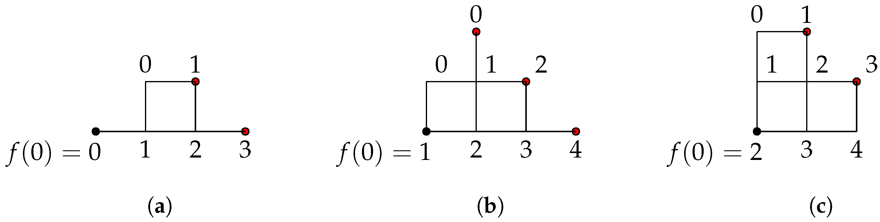
to count the shortest paths on square lattices. Figure 1a–c show the possible homomorphisms from

P_{4}

to

P_{5}

, which map 0 to 0, 1, and 2, respectively. The numbers on the top are elements of the domain set

V (P_{4})

, and the tuples on the left are elements of the image set

V (P_{5})

. These become square lattices, as shown in Figure 2a–c after rotating

45^{\circ}

counterclockwise.

Each homomorphism

f \in Hom (P_{m}, P_{n}) |

can be visualized using the square lattice, where movement from

(i, j)

to the next point is depicted as follows:

To $(i + 1, j)$ if $f (x + 1) = f (x) + 1$ .
To $(i, j + 1)$ , if $f (x + 1) = f (x) - 1$ .

For example, if the images of successive vertices of

f \in | {Hom}^{3} (P_{17}, P_{10}) |

are

3, 4

,

5, 4, 5, 4, 3, 2,

1, 0, 1, 2, 3, 2, 3, 4

and 5, then the homomorphism can be visualized as shown in Figure 3.

In general,

| {Hom}^{j} (P_{m}, P_{n}) |

can be obtained from the number of shortest paths from

(0, 0)

to any point

(i, n - i - 1)

on the square lattice that stays between the lines

y = x + j

and

y = x - n + j + 1

, where touching is allowed.

Lemma 2

([5]). The number of shortest paths from point

(0, 0)

to any point

(i, n - i - 1)

on the square lattice that stays between the lines

y = x + j

and

y = x - (n - j - 1)

is

\sum_{| t | \leq ⌊ (m + n) / n ⌋} ((\binom{m - 1}{i - t (n + 1)}) - (\binom{m - 1}{i + j - t (n + 1) + 1})) .

(3)

where

(\binom{n}{k}) = 0

if

k > n

or

k < 0

.

Hence, we obtain the following theorem.

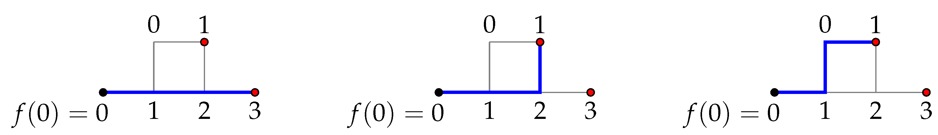
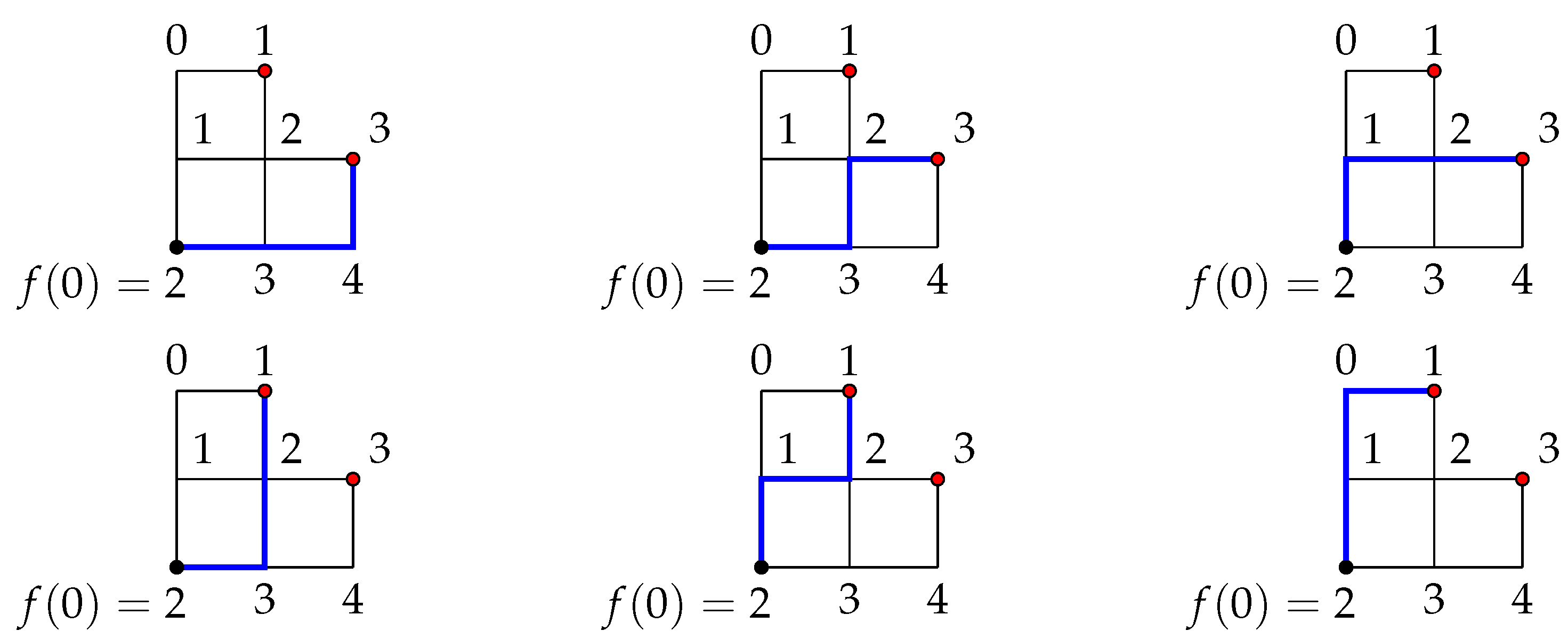
Theorem 1.

Let

m, n

be positive integers and j be a non-negative integer. Let

L = max {0,

⌈ \frac{m - j - 1}{2} ⌉}

and

U = min {m - 1, ⌊ \frac{m + n - j - 2}{2} ⌋}

. Then,

| {Hom}^{j} (P_{m}, P_{n}) | = \sum_{i = L}^{U} \sum_{| t | \leq ⌊ \frac{m + n}{n} ⌋} ((\binom{m - 1}{i - t (n + 1)}) - (\binom{m - 1}{i + j - t (n + 1) + 1}))

(4)

Example 1.

Using Theorem 1, we have

\begin{matrix} | {Hom}^{0} (P_{4}, P_{5}) | = & \sum_{i = 2}^{3} \sum_{t = - 1}^{1} ((\binom{3}{i - 6 t}) - (\binom{3}{i - 6 t + 1})) \\ = & \sum_{i = 2}^{3} ((\binom{3}{i + 6}) - (\binom{3}{i + 7}) + (\binom{3}{i}) - (\binom{3}{i + 1}) + (\binom{3}{i - 6}) - (\binom{3}{i - 5})) \\ = & ((\binom{3}{2}) - (\binom{3}{3})) + ((\binom{3}{3})) \\ = & 3, \end{matrix}

\begin{matrix} | {Hom}^{1} (P_{4}, P_{5}) | = & \sum_{i = 1}^{3} \sum_{t = - 1}^{1} ((\binom{3}{i - 6 t}) - (\binom{3}{i - 6 t + 2})) \\ = & \sum_{i = 1}^{3} ((\binom{3}{i + 6}) - (\binom{3}{i + 8}) + (\binom{3}{i}) - (\binom{3}{i + 2}) + (\binom{3}{i - 6}) - (\binom{3}{i - 4})) \\ = & ((\binom{3}{1}) - (\binom{3}{3})) + ((\binom{3}{2})) + ((\binom{3}{3})) \\ = & 6, \end{matrix}

and

\begin{matrix} | {Hom}^{2} (P_{4}, P_{5}) | = & \sum_{i = 1}^{2} \sum_{t = - 1}^{1} ((\binom{3}{i - 6 t}) - (\binom{3}{i - 6 t + 3})) \\ = & \sum_{i = 1}^{2} ((\binom{3}{i + 6}) - (\binom{3}{i + 9}) + (\binom{3}{i}) - (\binom{3}{i + 3}) + (\binom{3}{i - 6}) - (\binom{3}{i - 3})) \\ = & ((\binom{3}{1})) + ((\binom{3}{2})) \\ = & 6 . \end{matrix}

which is in line with counting directly from Figure 2. By counting the paths in Figure 2a, we have

| {Hom}^{0} (P_{4}, P_{5}) | = 3

(see Figure 4). By counting the paths in Figure 2b, we have

| {Hom}^{1} (P_{4}, P_{5}) | = 6

(see Figure 5). By counting the paths in Figure 2c, we have

| {Hom}^{2} (P_{4}, P_{5}) | = 6

. (see Figure 6).

For convenience, we compute

| {Hom}^{j} (P_{m}, P_{n}) |

for

2 \leq m, n \leq 9

(Table 1).

3. The Number of Homomorphisms from Paths to Rectangular Grid Graphs

In this section, we provide the formulas for finding the number of homomorphisms from paths

P_{m}

to rectangular grid graphs

P_{n} □ P_{k}

. We denote the set of homomorphisms from

P_{m}

to

P_{n} □ P_{k}

, which maps 0 to

(i, j)

, by

{Hom}^{i j} (P_{m}, P_{n} □ P_{k})

.

For

0 \leq i \leq n - 1

,

0 \leq j \leq k - 1

, let

{Hom}^{i j} (P_{m}, P_{n} □ P_{k}) = {f \in Hom (P_{m}, P_{n} □ P_{k}) ∣ f (0) = (i, j)} .

(5)

From the symmetry of

P_{n} □ P_{k}

, we obtain the following lemma:

Lemma 3.

Let i and n be integers such that

0 \leq j < n

, and let

m > 2

be a positive integer.

(1): $| {Hom}^{i j} (P_{m}, P_{n} □ P_{k}) | = | {Hom}^{(n - i - 1) j} (P_{m}, P_{n} □ P_{k}) | = | {Hom}^{i (k - j - 1)} (P_{m}, P_{n} □ P_{k}) |$
$= | {Hom}^{(n - i - 1) (k - j - 1)} (P_{m}, P_{n} □ P_{k}) |$ ,
for all $i \in {0, 1, \dots, n - 1}$ and $j \in {0, 1, \dots, k - 1}$ .
(2): $| Hom (P_{m}, P_{2 n} □ P_{2 k}) | = 4 \sum_{i = 0}^{n - 1} \sum_{j = 0}^{k - 1} | {Hom}^{i j} (P_{m}, P_{2 n} □ P_{2 k}) |$ .
(3): $| Hom (P_{m}, P_{2 n + 1} □ P_{2 k}) | = 4 \sum_{i = 0}^{n - 1} \sum_{j = 0}^{k - 1} | {Hom}^{i j} (P_{m}, P_{2 n + 1} □ P_{2 k}) |$
$+ 2 \sum_{j = 0}^{k - 1} | {Hom}^{n j} (P_{m}, P_{2 n + 1} □ P_{2 k}) |$ .
(4): $| Hom (P_{m}, P_{2 n} □ P_{2 k + 1}) | = 4 \sum_{i = 0}^{n - 1} \sum_{j = 0}^{k - 1} | {Hom}^{i j} (P_{m}, P_{2 n} □ P_{2 k + 1}) |$
$+ 2 \sum_{i = 0}^{n - 1} | {Hom}^{i k} (P_{m}, P_{2 n} □ P_{2 k + 1}) |$ .
(5): $| Hom (P_{m}, P_{2 n + 1} □ P_{2 k + 1}) | = 4 \sum_{i = 0}^{n - 1} \sum_{j = 0}^{k - 1} | {Hom}^{i j} (P_{m}, P_{2 n + 1} □ P_{2 k + 1}) |$
                                $+ 2 \sum_{j = 0}^{k - 1} | {Hom}^{n j} (P_{m}, P_{2 n + 1} □ P_{2 k + 1}) |$
                                $+ 2 \sum_{i = 0}^{n - 1} | {Hom}^{i k} (P_{m}, P_{2 n + 1} □ P_{2 k + 1}) |$
                                $+ | {Hom}^{n k} (P_{m}, P_{2 n + 1} □ P_{2 k + 1}) |$ .

To prove the main theorem, we define a new operation for two paths with their edge labelings.

Definition 1.

Let

P_{m}^{ϕ}, P_{n}^{ψ}

be paths

P_{m}, P_{n}

with edge labelings ϕ and ψ. Define

P_{m}^{ϕ}

and

P_{n}^{ψ}

entwined or

P_{m}^{ϕ} ≬ P_{n}^{ψ}

as the set of all paths

P_{m + n - 1}

with edge labels from ϕ and ψ that preserve the sequential order of ϕ and ψ.

Example 2.

Consider paths

P_{4}

and

P_{3}

with injective edge labelings ϕ and ψ, as shown below.

This leads to the following lemma:

Lemma 4.

Let

P_{m}^{ϕ}, P_{n}^{ψ}

be paths with edge labelings. Then,

| P_{m} ≬ P_{n} | = (\binom{m + n - 2}{m - 1}) .

(6)

Proof.

It is easy to see that the number of ways to label

P_{m + n - 1}

is equal to the permutations of all

m + n - 2

edge labels with a fixed sequential order. □

Next, we observe a simple example to visualize homomorphisms from paths to rectangular grid graphs on a square lattice.

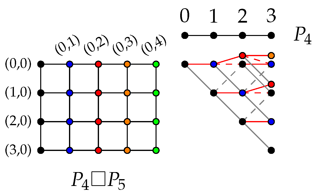
Example 3

(

{Hom}^{00} (P_{4}, P_{4} □ P_{5}) = 18

). All possible homomorphisms

f \in {Hom}^{00} (P_{4}, P_{4} □ P_{5})

are shown in Figure 7. The numbers on the top are elements of the domain set

V (P_{4})

, and the tuples on the left are elements of the image set

V (P_{4} □ P_{5})

. The tuples with the same second elements are represented by circles of the same color.

The mappings

f_{1}, f_{2} \in {Hom}^{00} (P_{4}, P_{4} □ P_{5})

with

f_{1} (0) = (0, 0), f_{1} (1) = (0, 1)

,

f_{1} (2) = (0, 2)

,

f_{1} (3) = (0, 1)

and

f_{2} (0) = (0, 0), f_{2} (1) = (1, 0), f_{2} (2) = (2, 0), f_{2} (3) = (1, 0)

are represented by the red lines on the top and the black lines (see Figure 8). We note that the normal black lines represent the increment of the first coordinate, the dashed black lines represent the decrement of the first coordinate, the normal red lines represent the increment of the second coordinate, and the red lines represent the decrement of the second coordinate.

We now divide all mappings in

{Hom}^{00} (P_{4}, P_{4} □ P_{5})

into groups according to the number of change occurrences in the first coordinate h and rewrite each path as entwined black and red paths. Mathematics 11 02587 i002

For each

h \in {0, 1, 2, 3}

, observe that out of the 3 edges of

P_{4}

from

P_{h + 1} ≬ P_{4 - h}

, there are

(\binom{3}{h})

ways to place h edges from the black path and one way to place

3 - h

edges from the red path. Moreover, the black line

P_{h + 1}

is the square lattice representation of

f_{1} \in {Hom}^{0} (P_{h + 1}, P_{4})

, while the red line

P_{4 - h}

is the square lattice representation of

f_{2} \in {Hom}^{0} (P_{4 - h}, P_{5})

. Thus, there are

(\binom{3}{h}) | {Hom}^{0} (P_{h + 1}, P_{4}) | | {Hom}^{0} (P_{4 - h}, P_{5}) |

possible paths in

P_{h + 1} ≬ P_{4 - h}

. Hence,

\begin{matrix} | {Hom}^{00} (P_{4}, P_{4} □ P_{5}) | & = (\binom{3}{0}) | {Hom}^{0} (P_{1}, P_{4}) | | {Hom}^{0} (P_{4}, P_{5}) | \\ + (\binom{3}{1}) | {Hom}^{0} (P_{2}, P_{4}) | | {Hom}^{0} (P_{3}, P_{5}) | \\ + (\binom{3}{2}) | {Hom}^{0} (P_{3}, P_{4}) | | {Hom}^{0} (P_{2}, P_{5}) | \\ + (\binom{3}{3}) | {Hom}^{0} (P_{4}, P_{4}) | {Hom}^{0} (P_{1}, P_{5}) | \\ = 1 (1) (3) + 3 (1) (2) + 3 (2) (1) + 1 (3) (1) \\ = 18 . \end{matrix}

Example 4

(

| {Hom}^{11} (P_{4}, P_{4} □ P_{5}) | = 47

). All possible homomorphisms

f \in {Hom}^{11} (P_{4}, P_{4} □ P_{5})

are shown in Figure 9. The numbers on the top are elements of the domain set

V (P_{4})

, and the tuples on the left are elements of the image set

V (P_{4} □ P_{5})

. The tuples with the same second elements are represented by circles of the same color.

\begin{matrix} | {Hom}^{11} (P_{4}, P_{4} □ P_{5}) | & = (\binom{3}{0}) | {Hom}^{1} (P_{1}, P_{4}) | | {Hom}^{1} (P_{4}, P_{5}) | \\ + (\binom{3}{1}) | {Hom}^{1} (P_{2}, P_{4}) | | {Hom}^{1} (P_{3}, P_{5}) | \\ + (\binom{3}{2}) | {Hom}^{1} (P_{3}, P_{4}) | | {Hom}^{1} (P_{2}, P_{5}) | \\ + (\binom{3}{3}) | {Hom}^{1} (P_{4}, P_{4}) | {Hom}^{1} (P_{1}, P_{5}) | \\ = 1 (1) (6) + 3 (2) (3) + 3 (3) (2) + 1 (5) (1) \\ = 47 . \end{matrix}

Lemma 5.

Let

m, n

and k be positive integers and let

i, j

be non-negative integers, such that

i < \frac{n}{2} - 1

and

j < \frac{k}{2} - 1

. It follows that

| {Hom}^{i j} (P_{m}, P_{n} □ P_{k}) | = \sum_{h = 0}^{m - 1} (\binom{m - 1}{h}) | {Hom}^{i} (P_{h + 1}, P_{n}) | | {Hom}^{j} (P_{m - h}, P_{k}) | .

(7)

Proof.

Let

f \in {Hom}^{i j} (P_{m}, P_{n} □ P_{k})

. For each

x \in {0, 1, m - 2}

in the domain, either

f (x + 1) = f (x) \pm (1, 0)

or

f (x + 1) = f (x) \pm (0, 1)

. Assume changes in the first coordinate appear h times. Then, changes in the second coordinate appear

m - 1 - h

times. The sequence of changes in the first coordinate form a homomorphism

f_{1} \in H o m^{i} (P_{h + 1}, P_{n})

. Similarly, the sequence of changes in the second coordinate form a homomorphism

f_{2} \in H o m^{i} (P_{m - 1 - h + 1}, P_{k})

. Thus, the corresponding path graph of f can be obtained from path graphs of

f_{1}

and

f_{2}

entwined. Hence,

| {Hom}^{i j} (P_{m}, P_{n} □ P_{k}) | = \sum_{h = 0}^{m - 1} (\binom{m - 1}{h}) | {Hom}^{i} (P_{h + 1}, P_{n}) | | {Hom}^{j} (P_{m - h}, P_{k}) | .

□

From Theorem 1, Lemma 3 and Lemma 5, we get the theorem below.

Theorem 2.

Let

m, n

and k be positive integers. The cardinalities

| Hom (P_{m}, P_{n} □ P_{k}) |

of homomorphisms from paths

P_{m}

to rectangular grid graphs

P_{n} □ P_{k}

are

| Hom (P_{m}, P_{n} □ P_{k}) | = 4 \sum_{i = 0}^{⌊ n / 2 ⌋ - 1} \sum_{j = 0}^{⌊ k / 2 ⌋ - 1} | {Hom}^{i j} (P_{m}, P_{n} □ P_{k}) |

+ (1 - {(- 1)}^{n}) \sum_{j = 0}^{⌊ k / 2 ⌋ - 1} | {Hom}^{⌊ n / 2 ⌋ j} (P_{m}, P_{n} □ P_{k}) |

+ (1 - {(- 1)}^{k}) \sum_{i = 0}^{⌊ n / 2 ⌋ - 1} | {Hom}^{i ⌊ k / 2 ⌋} (P_{m}, P_{n} □ P_{k}) |

+ (1 / 4) (1 - {(- 1)}^{n}) (1 - {(- 1)}^{k}) | {Hom}^{⌊ n / 2 ⌋ ⌊ k / 2 ⌋} (P_{m}, P_{n} □ P_{k}) |

where

| {Hom}^{i j} (P_{m}, P_{n} □ P_{k}) | = \sum_{h = 0}^{m - 1} (\binom{m - 1}{h}) | {Hom}^{i} (P_{h + 1}, P_{n}) | | {Hom}^{j} (P_{m - h}, P_{k}) |

and

\begin{matrix} | {Hom}^{j} (P_{m}, P_{n}) | = \sum_{i = L}^{U} \sum_{| t | \leq ⌊ \frac{m + n}{n} ⌋} ((\binom{m - 1}{i - t (n + 1)}) - (\binom{m - 1}{i + j - t (n + 1) + 1})), \end{matrix}

where

L = max {0, ⌈ \frac{m - j - 1}{2} ⌉}

and

U = min {m - 1, ⌊ \frac{m + n - j - 2}{2} ⌋}

.

For convenience, we compute

| Hom (P_{m}, P_{n} □ P_{k}) |

for

2 \leq m, n, k \leq 8

. The results are presented in Table 2.

4. The Algorithm

In this section, we provide algorithms used to calculate

| {Hom}^{i} (P_{m}, P_{n}) |

,

| {Hom}^{i j} (P_{m}, P_{n} □ P_{k}) |

and

| Hom (P_{m}, P_{n} □ P_{k}) |

with the aforementioned theorems.

Algorithms 1–3 are implementations of Theorem 1, Lemma 5 and Theorem 2, respectively.

Algorithm 1LocalPath2Path: Number of Homomorphisms from

P_{m}

to

P_{n}

with

f (0) = j

Input:

- m: the size of the domain

- n: the size of the range

- Fixed value j where

f (0) = j

(with

0 \leq j \leq n - 1

)

Output: number of homomorphisms from

P_{m}

to

P_{n}

with

f (0) = j

$L \leftarrow max {0, ⌈\frac{m - j - 1}{2}⌉}$
$U \leftarrow min {m - 1, ⌊\frac{m + n - j - 2}{2}⌋}$
if $L > U$ then
return 0
end if
$h o m j \leftarrow 0$
for $i = L$ to $U$ do
for $t = - ⌊\frac{m + n}{n}⌋$ to $⌊\frac{m + n}{n}⌋$ do
$h o m j \leftarrow h o m j + (\binom{m - 1}{i - t (n + 1)}) - (\binom{m - 1}{i + j - t (n + 1) + 1})$
end for
end for
return $h o m j$

Algorithm 2LocalPath2Grid: Number of Homomorphisms from

P_{m}

to

P_{n} □ P_{k}

with

f (0) = (i, j)

Input:

- m: the size of the domain

-

n, k

: the dimensions of the grid representing the range

- Fixed value

i, j

where

f (0) = (i, j)

(with

0 \leq i \leq n - 1

and

0 \leq j \leq k - 1

)

Output: number of homomorphisms from

P_{m}

to

P_{n} □ P_{k}

with

f (0) = (i, j)

$h o m i j \leftarrow 0$
for $h = 0$ to $m - 1$ do
$c_{i} \leftarrow L o c a l P a t h 2 P a t h (h + 1, n, i)$
$c_{j} \leftarrow L o c a l P a t h 2 P a t h (m - h, k, j)$
$h o m i j \leftarrow h o m i j + (\binom{m - 1}{h}) c_{i} c_{j}$
end for
return homij

Algorithm 3Path2Grid: Number of Homomorphisms from

P_{m}

to

P_{n} □ P_{k}

Input:

- m: the size of the domain

-

n, k

: the dimensions of the grid representing the range

Output: number of homomorphisms from

P_{m}

to

P_{n} □ P_{k}

$h o m g r i d \leftarrow 0$
$s u m \leftarrow 0$
for $i = 0$ to $⌊n / 2⌋ - 1$ do
for $j = 0$ to $⌊k / 2⌋ - 1$ do
$s u m \leftarrow s u m + L o c a l P a t h 2 G r i d (m, n, k, i, j)$
end for
end for
$h o m g r i d \leftarrow h o m g r i d + s u m * 4$
$s u m \leftarrow 0$
for $j = 0$ to $⌊k / 2⌋ - 1$ do
$s u m \leftarrow s u m + L o c a l P a t h 2 G r i d (m, n, k, ⌊n / 2⌋, j)$
end for
$h o m g r i d \leftarrow h o m g r i d + (1 - {(- 1)}^{n}) * s u m$
$s u m \leftarrow 0$
for $i = 0$ to $⌊n / 2⌋ - 1$ do
$s u m \leftarrow s u m + L o c a l P a t h 2 G r i d (m, n, k, i, ⌊k / 2⌋)$
end for
$h o m g r i d \leftarrow h o m g r i d + (1 - {(- 1)}^{k}) * s u m$
$h o m g r i d \leftarrow h o m g r i d + \frac{1}{4} (1 - {(- 1)}^{n}) (1 - {(- 1)}^{k}) L o c a l P a t h 2 G r i d (m, n, k, ⌊n / 2⌋, ⌊k / 2⌋)$
return $h o m g r i d$

Lemma 6.

Algorithm

P a t h 2 G r i d

has time-complexity

O (n \cdot m \cdot k \cdot max (n, m, k))

.

Proof.

It is easy to see that the complexity of the algorithm depends on the first loop, which is also nested with

O (n \cdot k)

rounds. Each round consists of an execution of LOCALPATH2GRID, which is essentially a loop with

O (m)

rounds. Each of these deeper rounds calls LOCALPATH2PATH twice.

To see the runtime for LOCALPATH2PATH given parameters m and n, we first see the complexity of the outer loop:

\begin{matrix} O (U - L) & = O (min \{m - 1, m - 1 - ⌈\frac{m - j - 1}{2}⌉, ⌊\frac{m + n - j - 2}{2}⌋, \\ ⌊\frac{m + n - j - 2}{2}⌋ - ⌈\frac{m - j - 1}{2}⌉\}) \\ \leq O (min \{m, m + n, n\}) = O (min {m, n}) \end{matrix}

(8)

Then, we consider the following scenarios:

$m < n$ : In this case $⌊(m + n) / n⌋ = 1$ ; hence, the inner loop has fixed rounds. Therefore, the complexity is at most $O (min {m, n})$ .
$m > = n$ : In this case, the complexity of the inner loop is $O (⌊ (m + n) / n ⌋)$ . Together, we have the overall complexity:

$\begin{matrix} O (min {m, n}) O (⌊ (m + n) / n ⌋) & = O (n) O (⌊ (m + n) / n ⌋) \\ \leq O (n) O (m / n) \\ \leq O (m) \end{matrix}$

(9)

Therefore, the overall complexity of LOCALPATH2PATH is

O (min {m, n})

. Since each round of LOCALPATH2GRID calls LOCALPATH2PATH twice, respectively with parameters

(h + 1, n)

and

(m - h, k)

, we have its complexity as:

\begin{matrix} O (min {h + 1, n}) + O (min {m - h, k}) \\ \leq O (min {m, n}) + O (min {m, k}) \\ \leq O (max {m, n}) + O (max {m, k}) \\ \leq O (max {m, n, k}) \end{matrix}

(10)

Together, the total complexity of PATH2GRID is

O (m \cdot n \cdot k \cdot max {m, n, k})

. □

Author Contributions

Conceptualization, S.P.; methodology, S.P.; software, H.Y.; validation, H.Y.; investigation, P.R.; writing—original draft, P.R.; writing—review and editing, H.Y. and S.P.; visualization, H.Y. and P.R.; project administration, S.P.; funding acquisition, S.P. All authors have read and agreed to the published version of the manuscript.

Funding

This research was funded by Chiang Mai University.

Data Availability Statement

Data sharing not applicable.

Acknowledgments

We thank the reviewers for their insightful comments and suggestions that improved the quality of our manuscript. We wish to express our thanks to Pham Hoang Viet for several helpful comments concerning algorithm analyzing. This research was supported by Faculty of Science, Chiang Mai University, and Chiang Mai University, Thailand.

Conflicts of Interest

The authors declare no conflict of interest.

References

Hell, P.; Nestril, J. Graphs and Homomorphisms; Oxford University Press: Oxford, UK, 2004. [Google Scholar]
Knauer, U.; Knauer, K. Algebraic Graph Theory: Morphisms, Monoids and Matrices; Walter de Gruyter: Berlin, Germany, 2011. [Google Scholar]
Arworn, S. An algorithm for the numbers of endomorphisms on paths. Discret. Math. 2009, 309, 94–103. [Google Scholar] [CrossRef] [Green Version]
Arworn, S.; Wojtylak, P. An algorithm for the number of path homomorphisms. Discret. Math. 2009, 309, 5569–5573. [Google Scholar] [CrossRef] [Green Version]
Lina, Z.; Zeng, J. On the number of congruence classes of paths. Discret. Math. 2012, 312, 1300–1307. [Google Scholar] [CrossRef] [Green Version]
Michels, M.A.; Knauer, U.H. The congruence classes of paths and cycles. Discret. Math. 2009, 309, 5352–5359. [Google Scholar] [CrossRef] [Green Version]
Eggleton, R.B.; Morayne, M. A Note on Counting Homomorphisms of Paths. Graphs Comb. 2014, 30, 159–170. [Google Scholar] [CrossRef] [Green Version]
Knauer, U.; Pipattanajinda, N. A formula for the number of weak endomorphisms on paths. Algebra Discret. Math. 2018, 26, 270–279. [Google Scholar]
Pomsri, T.; Wannasit, W.; Panma, S. Finding the Number of Weak Homomorphisms of Paths. J. Math. 2022, 2022, 2153927. [Google Scholar] [CrossRef]
Keshavarz-Kohjerdi, F.; Bagheri, A. Finding Hamiltonian cycles of truncated rectangular grid graphs in linear time. Appl. Math. Comput. 2023, 436, 127513. [Google Scholar] [CrossRef]

Figure 1. Graphical presentation of the domain and image of all possible homomorphisms

f \in Hom

(P_{4}, P_{5})

. (a)

f (0) = 0

. (b)

f (0) = 1

. (c)

f (0) = 2

.

Figure 1. Graphical presentation of the domain and image of all possible homomorphisms

f \in Hom

(P_{4}, P_{5})

. (a)

f (0) = 0

. (b)

f (0) = 1

. (c)

f (0) = 2

.

Figure 2. Square lattice presentations of all possible homomorphisms

f \in Hom (P_{4}, P_{5})

. (a)

f (0) = 0

. (b)

f (0) = 1

. (c)

f (0) = 2

.

Figure 2. Square lattice presentations of all possible homomorphisms

f \in Hom (P_{4}, P_{5})

. (a)

f (0) = 0

. (b)

f (0) = 1

. (c)

f (0) = 2

.

Figure 3. The shortest path from (0, 0) to (9, 7) that stays between lines

y = x + j

and

y = x - n + j + 1

, where

j = 3

,

m = 17

and

n = 10

.

Figure 3. The shortest path from (0, 0) to (9, 7) that stays between lines

y = x + j

and

y = x - n + j + 1

, where

j = 3

,

m = 17

and

n = 10

.

Figure 4. All possible presentations of homomorphisms

f \in {Hom}^{0} (P_{4}, P_{5})

on a square lattice.

Figure 4. All possible presentations of homomorphisms

f \in {Hom}^{0} (P_{4}, P_{5})

on a square lattice.

Figure 5. All possible presentations of homomorphisms

f \in {Hom}^{1} (P_{4}, P_{5})

on a square lattice.

Figure 5. All possible presentations of homomorphisms

f \in {Hom}^{1} (P_{4}, P_{5})

on a square lattice.

Figure 6. All possible presentations of homomorphisms

f \in {Hom}^{2} (P_{4}, P_{5})

on a square lattice.

Figure 6. All possible presentations of homomorphisms

f \in {Hom}^{2} (P_{4}, P_{5})

on a square lattice.

Figure 7. Graphical presentation of the domain and image of all possible homomorphisms

f \in {Hom}^{00}

(P_{4}, P_{4} □ P_{5})

.

Figure 7. Graphical presentation of the domain and image of all possible homomorphisms

f \in {Hom}^{00}

(P_{4}, P_{4} □ P_{5})

.

Figure 8. Square lattice presentation of

f_{1}

and

f_{2}

.

Figure 8. Square lattice presentation of

f_{1}

and

f_{2}

.

Figure 9. Graphical presentation of the domain and image of all possible homomorphisms

f \in {Hom}^{11}

(P_{4}, P_{4} □ P_{5})

.

Figure 9. Graphical presentation of the domain and image of all possible homomorphisms

f \in {Hom}^{11}

(P_{4}, P_{4} □ P_{5})

.

Table 1. Numbers of homomorphisms

f \in {Hom}^{j} (P_{m}, P_{n})

for

2 \leq m, n \leq 9 .

Table 1. Numbers of homomorphisms

f \in {Hom}^{j} (P_{m}, P_{n})

for

2 \leq m, n \leq 9 .

		n
$m$	$j$	2	3	4	5	6	7	8
2	0	1	1	1	1	1	1	1
	1	1	2	2	2	2	2	2
	2	0	1	2	2	2	2	2
	3	0	0	1	2	2	2	2
3	0	1	2	2	2	2	2	2
	1	1	2	3	3	3	3	3
	2	0	2	3	4	4	4	4
	3	0	0	2	3	4	4	4
4	0	1	2	3	3	3	3	3
	1	1	2	5	6	6	6	6
	2	0	2	5	6	7	7	7
	3	0	0	3	6	7	8	8
5	0	1	4	5	6	6	6	6
	1	1	4	8	9	10	10	10
	2	0	4	8	12	13	14	14
	3	0	0	5	9	13	14	15
6	0	1	4	8	9	10	10	10
	1	1	8	13	18	19	20	20
	2	0	4	13	18	23	24	25
	3	0	0	8	18	23	28	29
7	0	1	8	13	18	19	20	20
	1	1	8	21	27	33	34	35
	2	0	8	21	36	42	48	49
	3	0	0	13	27	42	48	54
8	0	1	8	21	27	33	34	35
	1	1	16	34	54	61	68	69
	2	0	8	34	54	75	82	89
	3	0	0	21	54	75	96	103

Table 2. Numbers of homomorphisms

f \in (P_{m}, P_{n} □ P_{k})

for

2 \leq m \leq n, k \leq 8 .

Table 2. Numbers of homomorphisms

f \in (P_{m}, P_{n} □ P_{k})

for

2 \leq m \leq n, k \leq 8 .

		k
$m$	$n$	2	3	4	5	6	7	8
2	2	8	14	20	26	32	38	44
	3	14	24	34	44	54	64	74
	4	20	34	48	62	76	90	104
	5	26	44	62	80	98	116	134
	6	32	54	76	98	120	142	164
	7	38	64	90	116	142	168	194
	8	44	74	104	134	164	194	224
3	3	34	68	102	136	170	204	238
	4	52	102	152	202	252	302	352
	5	70	136	202	268	334	400	466
	6	88	170	252	334	416	498	580
	7	106	204	302	400	498	596	694
	8	124	238	352	466	580	694	808
4	4	136	308	488	668	848	1028	1208
	5	190	424	668	912	1156	1400	1644
	6	244	540	848	1156	1464	1772	2080
	7	298	656	1028	1400	1772	2144	2516
	8	352	772	1208	1644	2080	2516	2952
5	5	518	1330	2226	3132	4038	4944	5850
	6	680	1726	2876	4038	5200	6362	7524
	7	842	2122	3526	4944	6362	7780	9198
	8	1004	2518	4176	5850	7524	9198	10872
6	6	1900	5528	9788	14172	18568	22964	27360
	7	2386	6880	12138	17544	22964	28384	33804
	8	2872	8232	14488	20916	27360	33804	40248
7	7	6774	22360	41884	62454	83196	103952	124708
	8	8232	26976	50384	75020	99856	124708	149560
8	8	23628	88496	175476	269596	365328	461288	557264

Disclaimer/Publisher’s Note: The statements, opinions and data contained in all publications are solely those of the individual author(s) and contributor(s) and not of MDPI and/or the editor(s). MDPI and/or the editor(s) disclaim responsibility for any injury to people or property resulting from any ideas, methods, instructions or products referred to in the content.

© 2023 by the authors. Licensee MDPI, Basel, Switzerland. This article is an open access article distributed under the terms and conditions of the Creative Commons Attribution (CC BY) license (https://creativecommons.org/licenses/by/4.0/).

Share and Cite

MDPI and ACS Style

Yingtaweesittikul, H.; Panma, S.; Rochanakul, P. An Algorithm for the Numbers of Homomorphisms from Paths to Rectangular Grid Graphs. Mathematics 2023, 11, 2587. https://doi.org/10.3390/math11112587

AMA Style

Yingtaweesittikul H, Panma S, Rochanakul P. An Algorithm for the Numbers of Homomorphisms from Paths to Rectangular Grid Graphs. Mathematics. 2023; 11(11):2587. https://doi.org/10.3390/math11112587

Chicago/Turabian Style

Yingtaweesittikul, Hatairat, Sayan Panma, and Penying Rochanakul. 2023. "An Algorithm for the Numbers of Homomorphisms from Paths to Rectangular Grid Graphs" Mathematics 11, no. 11: 2587. https://doi.org/10.3390/math11112587

Note that from the first issue of 2016, this journal uses article numbers instead of page numbers. See further details here.

Article Menu

An Algorithm for the Numbers of Homomorphisms from Paths to Rectangular Grid Graphs

Abstract

1. Introduction

2. The Number of Homomorphisms from Paths to Paths with f(0) = j

3. The Number of Homomorphisms from Paths to Rectangular Grid Graphs

4. The Algorithm

Author Contributions

Funding

Data Availability Statement

Acknowledgments

Conflicts of Interest

References

Share and Cite

Article Metrics

Article Access Statistics

Further Information

Guidelines

MDPI Initiatives

Follow MDPI

		n
$m$	$j$	2	3	4	5	6	7	8
2	0	1	1	1	1	1	1	1
	1	1	2	2	2	2	2	2
	2	0	1	2	2	2	2	2
	3	0	0	1	2	2	2	2
3	0	1	2	2	2	2	2	2
	1	1	2	3	3	3	3	3
	2	0	2	3	4	4	4	4
	3	0	0	2	3	4	4	4
4	0	1	2	3	3	3	3	3
	1	1	2	5	6	6	6	6
	2	0	2	5	6	7	7	7
	3	0	0	3	6	7	8	8
5	0	1	4	5	6	6	6	6
	1	1	4	8	9	10	10	10
	2	0	4	8	12	13	14	14
	3	0	0	5	9	13	14	15
6	0	1	4	8	9	10	10	10
	1	1	8	13	18	19	20	20
	2	0	4	13	18	23	24	25
	3	0	0	8	18	23	28	29
7	0	1	8	13	18	19	20	20
	1	1	8	21	27	33	34	35
	2	0	8	21	36	42	48	49
	3	0	0	13	27	42	48	54
8	0	1	8	21	27	33	34	35
	1	1	16	34	54	61	68	69
	2	0	8	34	54	75	82	89
	3	0	0	21	54	75	96	103

		n
$m$	$j$	2	3	4	5	6	7	8
2	0	1	1	1	1	1	1	1
	1	1	2	2	2	2	2	2
	2	0	1	2	2	2	2	2
	3	0	0	1	2	2	2	2
3	0	1	2	2	2	2	2	2
	1	1	2	3	3	3	3	3
	2	0	2	3	4	4	4	4
	3	0	0	2	3	4	4	4
4	0	1	2	3	3	3	3	3
	1	1	2	5	6	6	6	6
	2	0	2	5	6	7	7	7
	3	0	0	3	6	7	8	8
5	0	1	4	5	6	6	6	6
	1	1	4	8	9	10	10	10
	2	0	4	8	12	13	14	14
	3	0	0	5	9	13	14	15
6	0	1	4	8	9	10	10	10
	1	1	8	13	18	19	20	20
	2	0	4	13	18	23	24	25
	3	0	0	8	18	23	28	29
7	0	1	8	13	18	19	20	20
	1	1	8	21	27	33	34	35
	2	0	8	21	36	42	48	49
	3	0	0	13	27	42	48	54
8	0	1	8	21	27	33	34	35
	1	1	16	34	54	61	68	69
	2	0	8	34	54	75	82	89
	3	0	0	21	54	75	96	103

		n
$m$	$j$	2	3	4	5	6	7	8
2	0	1	1	1	1	1	1	1
	1	1	2	2	2	2	2	2
	2	0	1	2	2	2	2	2
	3	0	0	1	2	2	2	2
3	0	1	2	2	2	2	2	2
	1	1	2	3	3	3	3	3
	2	0	2	3	4	4	4	4
	3	0	0	2	3	4	4	4
4	0	1	2	3	3	3	3	3
	1	1	2	5	6	6	6	6
	2	0	2	5	6	7	7	7
	3	0	0	3	6	7	8	8
5	0	1	4	5	6	6	6	6
	1	1	4	8	9	10	10	10
	2	0	4	8	12	13	14	14
	3	0	0	5	9	13	14	15
6	0	1	4	8	9	10	10	10
	1	1	8	13	18	19	20	20
	2	0	4	13	18	23	24	25
	3	0	0	8	18	23	28	29
7	0	1	8	13	18	19	20	20
	1	1	8	21	27	33	34	35
	2	0	8	21	36	42	48	49
	3	0	0	13	27	42	48	54
8	0	1	8	21	27	33	34	35
	1	1	16	34	54	61	68	69
	2	0	8	34	54	75	82	89
	3	0	0	21	54	75	96	103