Differential and Time-Discrete SEIRS Models with Vaccination: Local Stability, Validation and Sensitivity Analysis Using Bulgarian COVID-19 Data

Abstract

Bulgaria has the lowest COVID-19 vaccination rate in the European Union and the second-highest COVID-19 mortality rate in the world. That is why we think it is important better to understand the reason for this situation and to analyse the development of the disease over time. In this paper, an extended time-dependent SEIRS model SEIRS-VB is used to investigate the long-term behaviour of the COVID-19 epidemic. This model includes vaccination and vital dynamics. To apply the SEIRS-VB model some numerical simulation tools have been developed and for this reason a family of time-discrete variants are introduced. Suitable inverse problems for the identification of parameters in discrete models are solved. A methodology is proposed for selecting a discrete model from the constructed family, which has the closest parameter values to these in the differential SEIRS-VB model. To validate the studied models, Bulgarian COVID-19 data are used. To obtain all these results for the discrete models a mathematical analysis is carried out to illustrate some biological properties of the differential model SEIRS-VB, such as the non-negativity, boundedness, existence, and uniqueness. Using the next-generation method, the basic reproduction number associated with the model in the autonomous case is defined. The local stability of the disease-free equilibrium point is studied. Finally, a sensitivity analysis of the basic reproduction number is performed.

1. Introduction

The first mathematical epidemiological model was created by Daniel Bernoulli modelling smallpox in 1766 (see [1]). However, it was not until 1927 that Kermack and McKendrick [2] introduced the SIR model for a more precise analysis of epidemic diseases. Nowadays, almost a hundred years later, SIR-type models are the most commonly used deterministic models to describe the COVID-19 epidemic, caused by severe acute respiratory syndrome coronavirus 2 (SARS-CoV-2). Actually, there are two different types of models: statistical and mathematical, and both approaches depend upon prior estimates as well as reliable data. Historical remarks and comparisons between both methods can be found in [3]. In the present paper we only use the mathematical deterministic approach, based on systems of non-linear differential equations which can be solved analytically or numerically. In these models, the host population is divided into different categories according to infection, vaccination, hospitalization, quarantine, etc. The dynamics of the infection in the categories are modelled by a Cauchy problem for a system of non-linear ordinary differential equations. Different epidemiological parameters are involved in the models as coefficients in the differential equations. If the values of these parameters are known, one could numerically solve the corresponding Cauchy problem. Unfortunately, when it comes to new viruses, as in the case of SARS-CoV-2, these parameters are unknown and their change over time cannot be determined. Of course, after a long enough period of time, based on the statistics, one can guess the values of some of the parameters. It is often assumed that some parameters do not change during the dominance of a particular variant of the virus or for a short period of time. However, this is not sufficient in general cases for the successful application of these models. At the same time, available databases contain information on the number of individuals in some of the categories in the models, for example, infected, vaccinated, recovered, deceased cases. In this way, various inverse problems arise that must be solved to determine all the parameters in the relevant model (see [4,5,6,7,8,9]). Only then, analysing the behaviour of the parameters over time, would it be possible to make an assumption about their change in the future and make realistic forecasts for the development of the epidemic.

A key role for the invasion and persistence of an infection in a new host population [10], i.e., for the duration of the epidemic, is played by the so-called basic reproduction number ${\Re }_0$. In deterministic models ${\Re }_0$ relates to the stability of the equilibrium points (in the more general case of models with non-linear incidence we refer to [11,12]). The classical SIR/SEIR and SEIRS (susceptible-exposed-infectious-recovered-susceptible) models with constant parameters, from a mathematical perspective, have an infinite number of equilibrium points. More precise models involving, for example, vital dynamics usually have a finite number of equilibrium points—the disease-free equilibrium and the endemic equilibriums. Then, the typical situation from a mathematical perspective is the following (see [13,14,15,16,17]). When ${\Re }_0<1$, the disease-free equilibrium is globally asymptotically stable. Therefore, the number of infected individuals tends to zero as time $t\to \infty$ and the epidemic subsides. If ${\Re }_0>1$, the disease-free equilibrium is unstable, but there exists a unique endemic equilibrium which is globally asymptotically stable. This means that the epidemic does not end, but the number of infected individuals tends to a non-zero constant as $t\to \infty$. In other words, the number of infected people will be approximately constant after a certain point in time and the outbreak will stop being a global emergency. A similar scenario is being observed with the current COVID-19 epidemic, although it is a much more complex process and its long-term behaviour cannot be described by a model with constant coefficients. SIR-based models with time-dependent coefficients are more suitable for this purpose. Official datasets contain information for the daily variation in the number of individuals in some categories. Based on these, various time-discrete analogues of the differential models have been introduced (see [18,19,20,21,22,23,24]). The time-discrete models with step size $h=1$ day provide two interpretations [25]. First, each quantity in the model $z_k=z\left(t_k\right)$ is expressed in days${}^{-1}$ or alternatively, $z_k=z\left(t_k\right)h$ is dimensionless, where $t_k$ is a fixed day of the time frame under consideration.

Recently, there has been a lot of interest in the construction of various integer- or fractional-order time-discrete variants of different deterministic models. To model the memory effects of the disease, different time-fractional models have been used (see, for example, refs. [26,27,28]). By default, the use of such non-local models requires larger refined datasets. They are also quite computationally expensive, which is why well-specialized numerical algorithms are required [29]. Currently, integer-order explicit or implicit time-discrete models have been used to the model COVID-19 epidemics. For example, time-continuous and time-discrete versions of the classical SIR model are discussed in [25]. Stability analysis, parameter identification and validation with Brazilian and UK COVID-19 data have been conducted. Some time-continuous and explicit time-discrete SEIR models with eventual linear feedback vaccination and partial re-susceptibility are studied in [30]. The stability of both the disease-free and the endemic equilibrium points is discussed. The proposed model is tested with Italian COVID-19 data. In [31], an implicit time-discrete SIR models is used for estimation of the basic reproduction number for the second wave of COVID-19 in Fiji. An implicit time-discrete SIR model is established in [32]. It showed that many of the desired properties of the time-continuous case are still valid in the time-discrete implicit case. An upper error estimate was also derived. The developed time-discrete SIR model was applied to COVID-19 data in Germany and Iran.

Replacing differential models with time-discrete ones raises several questions. What is the relationship between the values of the parameters in the time-discrete models with step size $h=1$ and the daily values of parameters in the differential model? More precisely, whether the parameter values found in the discrete model with $h=1$ by solving an appropriate inverse problem are close enough to the daily values of the parameters in the corresponding differential problem? The values of which parameters in the models can be assumed to be known based on the known statistics? The answer to the last question affects the answers to the previous two questions. This answer, on the one hand, depends on the correctness of the official data, and on the other hand, on the results of the sensitivity analysis of the input parameters. The sensitivity analysis could also provide an answer to another interesting question: which parameters have the greatest influence on the basic reproduction number? This, in turn, is extremely useful for developing a good vaccination strategy and adequate measures to limit the spread of the virus. For similar or different approaches to designing optimal vaccination strategies see [33] or [34], respectively, and the references therein.

In this article, we seek answers to the questions formulated above in the case of the SEIRS-VB model introduced in our previous work [4]. This is an extended SEIRS model with additional categories: V for susceptible vaccinated individuals and B for individuals with vaccine-induced immunity. The rest of the paper is organized as follows:

In Section 2, we briefly describe the differential SEIRS-VB model with time-dependent coefficients (see [4] for more details). It includes vaccination and vital dynamics. In Section 3, we consider a SEIRS-VB model with constant coefficients that can be used for short periods of time. By studying analytic properties we determine its positively invariant region. In Section 4, we find the disease-free equilibrium point (DFEP) of the same model. After this, using the proposed next-generation method we define the basic reproduction number ${\Re }_0$. The impact of ${\Re }_0$ on the local stability of the DFEP is studied in Section 5. In Section 6.1, to numerically solve the differential model SEIRS-VB, we construct a family of time-discrete SEIRS-VB models (difference schemes) and find sufficient conditions for the step size and parameters under which the model preserves the positivity property. Furthermore, in Section 6.2, bearing in mind the available data on the spread of SARS-CoV-2, we formulate an appropriate inverse problem. Then, we propose an algorithm to solve this problem and find the parameters in the suggested time-discrete models with a step size of 1. This allows us to compute the daily values of ${\Re }_0$. Validation of the SEIRS-VB models is presented in Section 7. We use reported COVID-19 data for Bulgaria to show that the suggested parameter identification method leads to biologically reasonable results. Then, we find that the time-discrete model form family (with a step size of 1) for which the computed parameter values are closest to the parameter values in the differential model with time-dependent coefficients. On the other hand, the obtained results show that the parameters values in the differential SEIRS-VB model and in the time-discrete model, realized through an explicit (forward) Euler method (with a step size of 1), are rather different. This observation deserves more serious attention. Let us note that there are some authors who use time-discrete models based on the explicit Euler method, omitting that in general this method is conditionally stable. Parameter sensitivity analysis of the basic reproduction number is conducted in Section 8. A discussion and conclusions are outlined in Section 9 and Section 10, respectively.

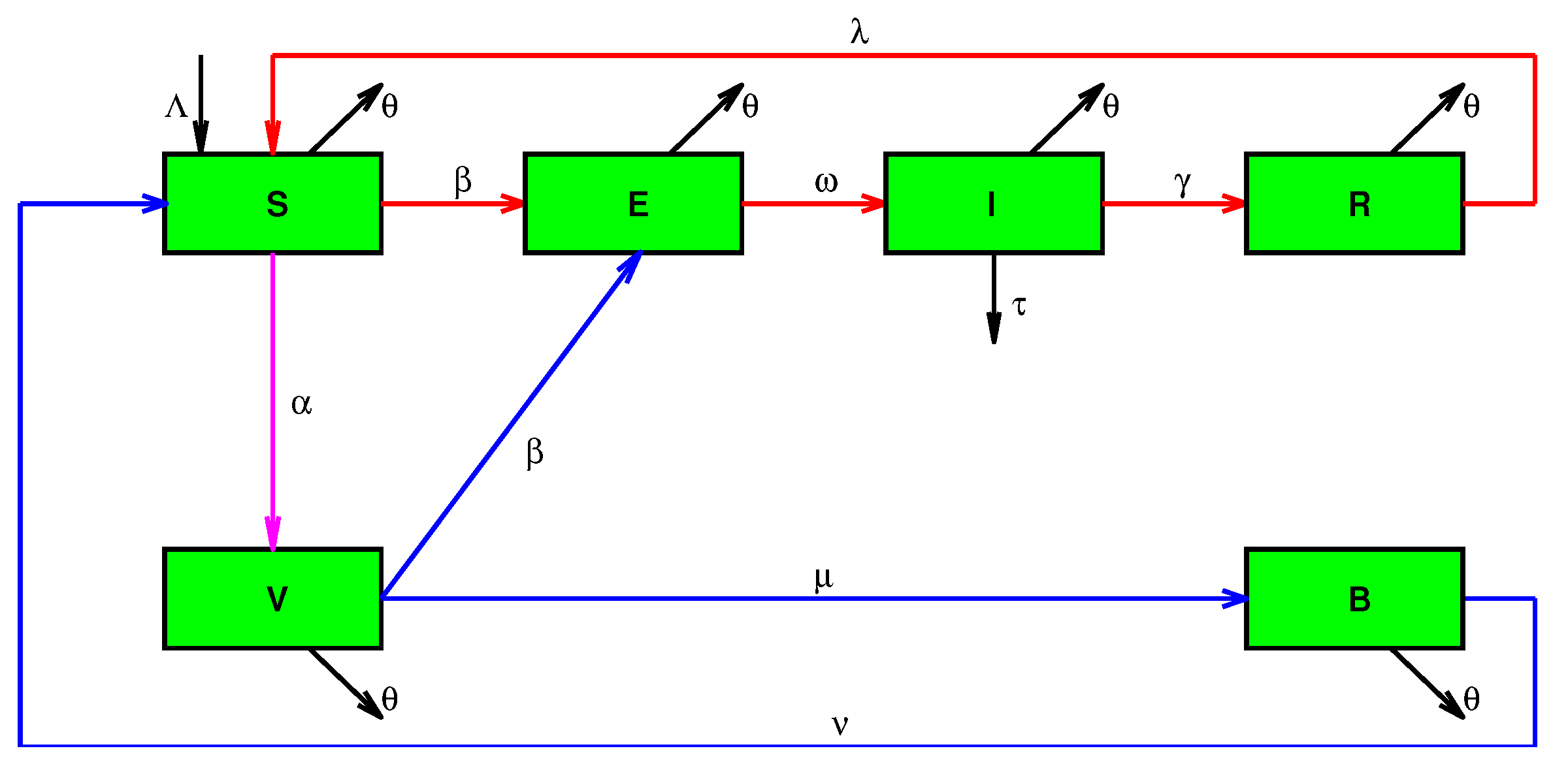
2. The Differential SEIR-VB Model

This paper deals with the mathematical modelling of COVID-19 transmission using the SEIRS-VB model, introduced in our previous work [4]. The model is described by the following Cauchy problem for a system of non-linear ordinary differential equations

$$\left|\begin{array}{c}{\displaystyle \frac{dS}{dt}=\mathrm{\Lambda }\left(t\right)N\left(t\right)-(\alpha \left(t\right)+\theta \left(t\right))S\left(t\right)-\frac{\beta \left(t\right)}{N\left(t\right)}S\left(t\right)I\left(t\right)+\lambda \left(t\right)R\left(t\right)+\nu \left(t\right)B\left(t\right),}\hfill \\ \\ {\displaystyle \frac{dE}{dt}=\frac{\beta \left(t\right)}{N\left(t\right)}S\left(t\right)I\left(t\right)+\frac{\beta \left(t\right)}{N\left(t\right)}V\left(t\right)I\left(t\right)-(\omega \left(t\right)+\theta \left(t\right))E\left(t\right),}\hfill \\ \\ {\displaystyle \frac{dI}{dt}=\omega \left(t\right)E\left(t\right)-(\gamma \left(t\right)+\tau \left(t\right)+\theta \left(t\right))I\left(t\right),}\hfill \\ \\ {\displaystyle \frac{dR}{dt}=\gamma \left(t\right)I\left(t\right)-(\lambda \left(t\right)+\theta \left(t\right))R\left(t\right),}\hfill \\ \\ {\displaystyle \frac{dV}{dt}=\alpha \left(t\right)S\left(t\right)-(\mu \left(t\right)+\theta \left(t\right))V\left(t\right)-\frac{\beta \left(t\right)}{N\left(t\right)}I\left(t\right)V\left(t\right),}\hfill \\ \\ {\displaystyle \frac{dB}{dt}=\mu \left(t\right)V\left(t\right)-(\nu \left(t\right)+\theta \left(t\right))B\left(t\right)}\hfill \end{array}\right.$$

(1)

with non-negative initial conditions

$$S\left(t_0\right)=S_0,E\left(t_0\right)=E_0,I\left(t_0\right)=I_0,R\left(t_0\right)=R_0,V\left(t_0\right)=V_0,B\left(t_0\right)=B_0,$$

(2)

where $t_0\ge 0$ is an integer number.

Here, the total population size is the number of all living individuals

$$N\left(t\right):=S\left(t\right)+E\left(t\right)+I\left(t\right)+R\left(t\right)+B\left(t\right)+V\left(t\right).$$

A full description of the SEIRS-VB model’s categories and parameters is given in [4]. Here, we will only note them briefly and give the model diagram in Figure 1:

Categories of the SEIRS-VB model:

• $S\left(t\right)$—susceptible individuals (unvaccinated, not fully vaccinated, vaccinated people for whom the vaccine is ineffective, fully vaccinated or recovered individuals who have lost their immunity).
• $E\left(t\right)$—exposed individuals. These are virus carriers in the latent stage, during which they are not virus spreaders. They usually have no symptoms.
• $I\left(t\right)$—infectious individuals. These are virus carriers and virus spreaders of extremely high infectivity. The former are likely to transmit the virus in case of contact.
• $R\left(t\right)$—Recovered individuals with disease-acquired immunity. These individuals have disease-acquired immunity. They have recovered, and thus are protected from the disease.
• $V\left(t\right)$—vaccinated susceptible individuals. These are fully vaccinated individuals for whom the vaccine is effective. However, they have not developed antibodies. They can do so after a certain period of time or otherwise they will become exposed individuals before that. It is worth pointing out that, due to vaccine imperfections, some of the vaccinated individuals cannot develop antibodies, and they cannot pass from group $S\left(t\right)$ to group $V\left(t\right)$.
• $B\left(t\right)$—vaccinated individuals with vaccination-acquired immunity. These are vaccinated individuals who are well protected from future infection because they have antibodies.

Parameters of the SEIRS-VB model:

• $\mathrm{\Lambda }\left(t\right)$—birth rate;
• $a\left(t\right)$—vaccination rate;
• $\sigma$—vaccine effectiveness;
• $\alpha \left(t\right)=\sigma a\left(t\right)$—vaccination parameter;
• $\beta \left(t\right)$—transmission rate;
• $\gamma \left(t\right)$—recovery rate;
• $\omega \left(t\right)$—latency rate;
• $\theta \left(t\right)$—natural mortality rate;
• $\tau \left(t\right)$—mortality rate of infectious people;
• $\lambda \left(t\right)$—reinfection rate of recovered individuals;
• $\nu \left(t\right)$—reinfection rate of vaccinated individuals;
• $\mu \left(t\right)$—antibody rate.

Available datasets contain daily numbers of individuals in some category in the SEIRS-BV model. In [4], using Bulgarian COVID-19 data we find daily values of the parameters in the model (1). In other words we assume that the parameters are step functions in time and for every single day we consider the problem (1) with constant coefficients. That is why, for simplicity, in the next three sections we study a SEIRS-VB model with time-independent coefficients, and define the basic reproduction number associated with it.

3. SEIRS-VB Model with Time-Independent Coefficients

To further introduce the basic reproduction number, in this section we begin by studying the simplified model with constant coefficients. To do this we analyse the disease-free equilibrium points (see explanation below) of the corresponding system of differential equations. Let us rewrite (1) using different notation

$$\left|\begin{array}{c}{\displaystyle \frac{dS}{dt}=\mathrm{\Omega }-(\alpha +\theta )S\left(t\right)-bS\left(t\right)I\left(t\right)+\lambda R\left(t\right)+\nu B\left(t\right),}\hfill \\ \\ {\displaystyle \frac{dE}{dt}=bS\left(t\right)I\left(t\right)+bV\left(t\right)I\left(t\right)-(\omega +\theta )E\left(t\right),}\hfill \\ \\ {\displaystyle \frac{dI}{dt}=\omega E\left(t\right)-(\gamma +\tau +\theta )I\left(t\right),}\hfill \\ \\ {\displaystyle \frac{dR}{dt}=\gamma I\left(t\right)-(\lambda +\theta )R\left(t\right),}\hfill \\ \\ {\displaystyle \frac{dV}{dt}=\alpha S\left(t\right)-(\mu +\theta )V\left(t\right)-bI\left(t\right)V\left(t\right),}\hfill \\ \\ {\displaystyle \frac{dB}{dt}=\mu V\left(t\right)-(\nu +\theta )B\left(t\right),}\hfill \end{array}\right.$$

(3)

where the new parameters are

$$\mathrm{\Omega }:=\mathrm{\Lambda }N>0,b:=\frac{\beta }{N}>0.$$

(4)

We suppose that all parameters $\mathrm{\Omega },b,\omega >0,\theta >0,\alpha \ge 0,\gamma \ge 0,\tau \ge 0,\nu \ge 0,\mu \ge 0$ are constants.

Remark 1.

Let us introduce the vector notations $X\left(t\right)=\left(S\right(t),E(t),I(t),R(t),V(t),B(t\left)\right)$, $X_0=(S_0,E_0,I_0,R_0,V_0,B_0)$, $N_0=S_0+E_0+I_0+R_0+V_0+B_0$, $p=(\alpha ,\beta ,\gamma ,\tau ,\mathrm{\Lambda },\theta ,\omega ,\lambda ,\mu ,\nu )$. Here and in the following we call a vector non-negative/positive if all its components are non-negative/positive.

Since the system (3) is a partial case of the SEIRS-VB model for the Cauchy problem (1), (2), we can apply the following theorem, proven in [4]:

Theorem 1.

(non-negativity, existence, uniqueness) [4] Let $X_0\ge 0$, $S_0>0,I_0>0$, $p\in C\left([t_0,T]\right)$ and $p\left(t\right)\ge 0,\mathrm{\Lambda }\left(t\right)>0,\beta \left(t\right)>0,\omega \left(t\right)>0$ for $t_0\le t\le T$. Then, there exists a solution $X\left(t\right)$ of the Cauchy problem (1), (2), which is defined for $t\in [t_0,T]$ and $X\left(t\right)\ge 0,$ $S\left(t\right)>0,I\left(t\right)>0$ for $t\in [t_0,T]$. The solution with such properties is unique.

We returned (see [10,35,36]) to the concept of the disease-free equilibrium point which means the equilibrium point $(S^{*},E^{*},I^{*},R^{*},V^{*},B^{*})$ of system (3), in which $E^{*}=0$ and $I^{*}=0$. We will use this equilibrium point to define the basic reproduction number ${\Re }_0$ associated with the model (3). We then find the daily ${\Re }_0$ values which are very important because they measure the transmission potential of a disease. Actually, the non-linear autonomous system (3) also has other equilibrium points, which are called endemic. However, the study of these points is not the subject of the present work, because they are only related to an autonomous system, not to a system with time-variable coefficients (1) used to model the long-term development of the COVID-19 epidemic.

Next, the following theorem gives a feasible region of the SEIRS-VB model (3).

Theorem 2.

(non-negativity, boundedness) A positively invariant set of the system (3) is

$$\Sigma :=\mathrm{\Psi }\cup \left\{X\ge 0:S>0,I>0,0<N\le \frac{\mathrm{\Omega }}{\theta }\right\},$$

(5)

where Ψ is the set of all disease-free equilibrium points of the system (3) with non-negative components.

Proof. 

Suppose $X_0\in \Sigma$:

Case 1. Let $X_0\in \mathrm{\Psi }$, i.e., $X_0$ is a disease-free equilibrium point of the system (3) with non-negative components. If $X\left(t\right)$ is a solution to (3) with $X\left(t_0\right)=X_0$, we have $X\left(t\right)=X_0\in \Sigma$ for all $t\ge t_0.$

Case 2. Let $X_0\in \Sigma \backslash \mathrm{\Psi }$, then for each arbitrary, but with fixed $T>0$, Theorem 1 implies that the unique solution $X\left(t\right)$ to the Cauchy problems (3) and (2) are defined in $[t_0,T]$ and $X\left(t\right)\ge 0,S\left(t\right)>0,I\left(t\right)>0$ and as a result $N\left(t\right)>0$ for $t\in [t_0,T].$

Adding the equations of the system (3) and initial conditions (2), we obtain

$$\left|\begin{array}{c}{\displaystyle \frac{dN\left(t\right)}{dt}=\mathrm{\Omega }-\theta N\left(t\right)-\tau I\left(t\right),}\hfill \\ \\ N\left(t_0\right)=N_0.\hfill \end{array}\right.$$

(6)

The unique solution of the Cauchy problem (6) is

$$N\left(t\right)=\frac{\mathrm{\Omega }}{\theta }+\left(N_0-\frac{\mathrm{\Omega }}{\theta }\right)e^{\theta (t_0-t)}-\tau e^{-\theta t}{\int }_{t_0}^t{e}^{\theta s}I\left(s\right)ds.$$

(7)

Since $I\left(t\right)>0$ for $t\in [t_0,T]$ and $N_0\le \mathrm{\Omega }/\theta$, we obtain

$$N\left(t\right)\le \frac{\mathrm{\Omega }}{\theta }.$$

Therefore, $X\left(t\right)\in \Sigma$ for $t\in [t_0,T]$.

The coefficients in the system (3) are constant. The number $T>0$ is arbitrary and therefore there exists a unique solution $X\left(t\right)$ of the system (3), defined as belonging to $\Sigma$ for all $t\ge t_0$. The proof is complete. □

4. The Disease-Free Equilibrium Point and Basic Reproduction Number

To find the disease-free equilibrium points of the autonomous system (3), we search for solutions ($S,E,I,R,V$ and B) with $E=0$ and $I=0$ of the system

$$\left|\begin{array}{c}\mathrm{\Omega }-(\alpha +\theta )S-bSI+\lambda R+\nu B=0,\hfill \\ \\ bSI+bVI-(\omega +\theta )E=0,\hfill \\ \\ \omega E-(\gamma +\tau +\theta )I=0,\hfill \\ \\ \gamma I-(\lambda +\theta )R=0,\hfill \\ \\ \alpha S-(\mu +\theta )V-bIV=0,\hfill \\ \\ \mu V-(\nu +\theta )B=0.\hfill \end{array}\right.$$

(8)

In this case, the system (3) becomes linear and has a unique disease-free equilibrium point

$$X^{*}:=(S^{*},E^{*},I^{*},R^{*},V^{*},B^{*})=\left(1,0,0,0,\frac{\alpha }{\mu +\theta },\frac{\alpha \mu }{(\mu +\theta )(\nu +\theta )}\right)S^{*},$$

(9)

where

$$S^{*}:=\frac{\mathrm{\Omega }(\nu +\theta )(\mu +\theta )}{\theta (\alpha \nu +(\mu +\theta \left)\right(\alpha +\nu +\theta \left)\right)}.$$

Remark 2.

We find that $\mathrm{\Psi }=X^{*}$ in (5) and $N^{*}=S^{*}+E^{*}+I^{*}+R^{*}+V^{*}+B^{*}=\mathrm{\Omega }/\theta$. Therefore, for all elements of $\Sigma$ we have the boundedness estimate $N\le \mathrm{\Omega }/\theta$ (see Theorem 2).

The Jacobian method (stability of the first approximation) is a widely used approach to derive a parameter that reflects the stability of the disease-free equilibrium. This parameter is used to establish the herd immunity threshold, but it sometimes does not yield the true value of the basic reproduction number. It is called the basic reproduction number if it has the same biological interpretation as the spectral radius of the next-generation matrix (see [35,36] and references therein). We find the basic reproduction number using the next-generation method and then using the Jacobian method to show that it is the stability parameter of the disease-free equilibrium.

Following [14,35], since we are concerned with the populations that spread the infection we only need to model the exposed E and infectious I categories. The dynamics in these two categories are modelled by the following equations

$$\left|\begin{array}{c}{\displaystyle \frac{dE}{dt}=bS\left(t\right)I\left(t\right)+bV\left(t\right)I\left(t\right)-(\omega +\theta )E\left(t\right),}\hfill \\ \\ {\displaystyle \frac{dI}{dt}=\omega E\left(t\right)-(\gamma +\tau +\theta )I\left(t\right).}\hfill \end{array}\right.$$

(10)

Let

$$F\left(X\right):={\left(b(S+V)I,0\right)}^T$$

be the rate of appearance of new infections in each category of (10),

$$W^{+}\left(X\right):={\left(0,\omega E\right)}^T$$

is the rate of transfer of individuals into each category of (10) by all other means and

$$W^{-}\left(X\right):={\left((\omega +\theta )E,(\gamma +\tau +\theta )I\right)}^T$$

is the rate of transfer of individuals from one category of (10).

Let us denote by $Y=(E,I)$ the group with infected individuals and reformulate the system (10) in the form

$$\frac{dY}{dt}=F-W,$$

(11)

where $W\left(X\right)=W^{-}\left(X\right)-W^{+}\left(X\right).$

Calculating the Jacobian matrix for F and W at the disease-free equilibrium point $X^{*}$, we obtain

$$\frac{\partial F}{\partial Y}\left(X^{*}\right):=\left(\begin{array}{cc}0& b(S^{*}+V^{*})\\ 0& 0\end{array}\right),\frac{\partial W}{\partial Y}\left(X^{*}\right):=\left(\begin{array}{cc}\omega +\theta & 0\\ -\omega & \gamma +\tau +\theta \end{array}\right).$$

Reminding (see [35,36]) that the next-generation matrix (operator) is defined by

$$G:=\frac{\partial F}{\partial Y}\left(X^{*}\right){\left(\frac{\partial W}{\partial Y}\left(X^{*}\right)\right)}^{-1}=\left(\begin{array}{cc}{\Re }_0& \frac{\omega +\theta }{\omega }{\Re }_0\\ 0& 0\end{array}\right),$$

where

$${\Re }_0:=\frac{\omega b(S^{*}+V^{*})}{(\omega +\theta )(\gamma +\tau +\theta )}=\frac{\omega b\mathrm{\Omega }(\nu +\theta )(\alpha +\mu +\theta )}{\theta (\omega +\theta )(\gamma +\tau +\theta )(\alpha \nu +(\mu +\theta \left)\right(\alpha +\nu +\theta \left)\right)}.$$

(12)

The eigenvalues of the matrix G are 0 and ${\Re }_0$. The basic reproduction number is defined as the spectral radius of the matrix G (the maximum absolute values of its eigenvalues), and is ${\Re }_0$. From a biological perspective the basic reproduction number is the number of secondary cases or new infections produced by a single infectious individual in a completely susceptible host population [13,36].

Remark 3.

We use this notation and definition in the case of constant coefficients in our method in Section 6, Section 7 and Section 8 for a fixed time period of one day, assuming that all parameters are appropriate constants and consequently our reproduction number ${\Re }_0$ is also constant. Of course, the values of ${\Re }_0$ depend on t and will differ for different days, making the basic reproduction number a step function ${\Re }_0\left(t\right)$.

5. Local Stability Analysis of the Disease-Free Equilibrium Point

Here we introduce the concept of the locally stable equilibrium point, meaning that any solution starting near that point will be near it all the time. More precisely, following Barbashin ([37], page 19), we call the equilibrium point $X^{*}$ of the system (8) locally stable on $\Sigma$ if for every $\epsilon >0$, there exists $\delta \left(\epsilon \right)>0$ such that for any other solution $X\left(t\right)$ of the system (8) on $\Sigma$ from the inequality $\left|\right|X\left(t_0\right)-X^{*}\left|\right|\le \delta \left(\epsilon \right)$, there follows $\left|\right|X\left(t\right)-X^{*}\left|\right|\le \epsilon$ for $t\ge t_0$. We call $X^{*}$ locally asymptotically stable on $\Sigma$ if it is locally stable on $\Sigma$ and there exists a positive number h, such that for $\left|\right|X\left(t_0\right)-X^{*}\left|\right|\le h$ we have $\left|\right|X\left(t\right)-X^{*}\left|\right|\to 0$ as $t\to +\infty$.

Now, we use this theory in the case of the disease-free equilibrium point $X^{*}$.

Theorem 3.

Let the coefficients of the system (3) be non-negative and $\omega >0,\theta >0,\mathrm{\Omega }>0.$ If ${\Re }_0<1$, then the disease-free equilibrium point $X^{*}$ of the system (3) is locally asymptotically stable on Σ. If ${\Re }_0>1,$ then the point $X^{*}$ is locally unstable on Σ.

Proof. 

The Jacobian matrix of (3) evaluated at the disease-free equilibrium point $X^{*}$ is

$$J\left(X^{*}\right)=\left(\begin{array}{cccccc}-\alpha -\theta & 0& -b{S}^{*}& \lambda & 0& \nu \\ 0& -\omega -\theta & b(S^{*}+V^{*})& 0& 0& 0\\ 0& \omega & -\gamma -\tau -\theta & 0& 0& 0\\ 0& 0& \gamma & -\lambda -\theta & 0& 0\\ \alpha & 0& -b{V}^{*}& 0& -\mu -\theta & 0\\ 0& 0& 0& 0& \mu & -\nu -\theta \end{array}\right).$$

It is easy to calculate that the characteristic polynomial $P\left(\zeta \right)$ of $J\left(X^{*}\right)$ has the following representation

$$\begin{array}{c}\hfill P\left(\zeta \right)=P_1\left(\zeta \right)P_2\left(\zeta \right),\end{array}$$

where

$$P_1\left(\zeta \right):=(\lambda +\theta +\zeta )(\theta +\zeta )\left\{{(\theta +\zeta )}^2+(\nu +\mu +\alpha )(\theta +\zeta )+\alpha \mu +\alpha \nu +\mu \nu \right\}$$

and

$$P_2\left(\zeta \right):={\zeta }^2+(\omega +\gamma +\tau +2\theta )\zeta +(\omega +\theta )(\gamma +\tau +\theta )(1-{\Re }_0).$$

The polynomial $P_1\left(\zeta \right)$ has four roots ${\zeta }_1,{\zeta }_2,{\zeta }_3,{\zeta }_4$, where ${\zeta }_1=-\theta <0$ and ${\zeta }_2=-\lambda -\theta <0$. The last two roots ${\zeta }_3$ and ${\zeta }_4$ satisfy

$${\zeta }_3+{\zeta }_4=-(\nu +\mu +\alpha )-2\theta <0,({\zeta }_3+\theta )({\zeta }_4+\theta )=\alpha \mu +\alpha \nu +\mu \nu >0.$$

Hence, the roots of $P_1\left(\zeta \right)$ have negative real parts.

Similar arguments for the roots ${\zeta }_5$ and ${\zeta }_6$ of the other polynomials $P_2\left(\zeta \right)$ give

$${\zeta }_5+{\zeta }_6=-(\omega +\gamma +\tau +2\theta )<0,{\zeta }_5{\zeta }_6=(\omega +\theta )(\gamma +\tau +\theta )(1-{\Re }_0).$$

If ${\Re }_0<1$, then ${\zeta }_5$ and ${\zeta }_6$ have negative real parts. According to the stability theorem of the first approximation (Theorem 11.1 in [37], p. 45) $X^{*}$ is locally asymptotically stable on $\Sigma$. If ${\Re }_0>1$, then one of the eigenvalues ${\zeta }_5$ or ${\zeta }_6$ is positive and according to the instability theorem of the first approximation (Theorem 11.2 in [37], p. 45) $X^{*}$ is locally unstable.

The proof is complete. □

Remark 4.

It is possible to study the impact of the basic reproduction number ${\Re }_0$ on the global asymptotic stability of the disease-free equilibrium point $X^{*}$ and the epidemic equilibrium points (with $I^{*}{E}^{*}\ne 0$) of the autonomous SEIRS-VB model (3). Commonly used methods to perform a global stability analysis are the method of Carlos Castillo-Chavez [14,38,39] and the direct Lyapunov method [12,15,37,40]. However, this would be of no practical importance because the long-term behaviour of a complex real-world process such as the COVID-19 epidemic cannot be described by models with constant parameters. For this reason, as already noted, we applied the autonomous system (3) to describe the daily changes in the number of individuals in different categories in the SEIRV-BD model. The results are step functions, as are the available data.

6. Time-Discrete SEIRS-VB Model

6.1. Construction of a New Family of Semi-Implicit Difference Schemes

In this section, we introduce a new family of semi-implicit difference schemes as time-discrete analogues of the differential model SEIRS-VB (1).

We consider the time-frame $t_1,t_2,\dots ,t_K$, where $t_0\le t_1<t_2<\dots <t_K\le T$ and introduce the notation for the values of functions

$$X_k:=(S_k,E_k,I_k,R_k,V_k,B_k)=(S\left(t_k\right),E\left(t_k\right),I\left(t_k\right),R\left(t_k\right),V\left(t_k\right),B\left(t_k\right)),$$

$$N_k:=N\left(t_k\right)=S_k+E_k+I_k+R_k+V_k+B_k,$$

for $k=1,2,\dots ,K$ and the values of the parameters

$$\begin{array}{cc}\hfill p_k& :=({\alpha }_k,{\beta }_k,{\gamma }_k,{\tau }_k,{\mathrm{\Lambda }}_k,{\theta }_k,{\omega }_k,{\lambda }_k,{\mu }_k,{\nu }_k)\hfill \\ & =(\alpha \left(t_k\right),\beta \left(t_k\right),\gamma \left(t_k\right),\tau \left(t_k\right),\mathrm{\Lambda }\left(t_k\right),\theta \left(t_k\right),\omega \left(t_k\right),\lambda \left(t_k\right),\mu \left(t_k\right),\nu \left(t_k\right)),\hfill \end{array}$$

$k=1,2,\dots ,K-1.$

Starting with the given initial data $S\left(t_1\right)=S_1,E\left(t_1\right)=E_1,I\left(t_1\right)=I_1,R\left(t_1\right)=R_1,$$V\left(t_1\right)=V_1,B\left(t_1\right)=B_1$ we consider the following family of time-discrete models with weights $0\le \xi \le 1$, $0\le \eta \le 1$:

$$\left|\begin{array}{c}\begin{array}{cc}\hfill {\displaystyle \frac{S_k-S_{k-1}}{h}=}& {\mathrm{\Lambda }}_{k-1}{N}_{k-1}-({\alpha }_{k-1}+{\theta }_{k-1})S_{k-1}-\frac{{\beta }_{k-1}}{N_{k-1}}{S}_{k-1}[(1-\xi )I_{k-1}+\xi I_k]+{\lambda }_{k-1}{R}_{k-1}+{\nu }_{k-1}{B}_{k-1},\hfill \\ \\ \hfill {\displaystyle \frac{E_k-E_{k-1}}{h}=}& \frac{{\beta }_{k-1}}{N_{k-1}}(S_{k-1}+V_{k-1})[(1-\xi )I_{k-1}+\xi I_k]-({\omega }_{k-1}+{\theta }_{k-1})E_{k-1},\hfill \\ \\ \hfill {\displaystyle \frac{I_k-I_{k-1}}{h}=}& {\omega }_{k-1}{E}_{k-1}-({\gamma }_{k-1}+{\tau }_{k-1})[(1-\eta )I_{k-1}+\eta I_k]-{\theta }_{k-1}{I}_{k-1},\hfill \\ \\ \hfill {\displaystyle \frac{R_k-R_{k-1}}{h}=}& {\gamma }_{k-1}[(1-\eta )I_{k-1}+\eta I_k]-({\lambda }_{k-1}+{\theta }_{k-1})R_{k-1},\hfill \\ \\ \hfill {\displaystyle \frac{V_k-V_{k-1}}{h}=}& {\alpha }_{k-1}{S}_{k-1}-\frac{{\beta }_{k-1}}{N_{k-1}}{V}_{k-1}[(1-\xi )I_{k-1}+\xi I_k]-({\mu }_{k-1}+{\theta }_{k-1})V_{k-1},\hfill \\ \\ \hfill {\displaystyle \frac{B_k-B_{k-1}}{h}=}& {\mu }_{k-1}{V}_{k-1}-({\nu }_{k-1}+{\theta }_{k-1})B_{k-1},\hfill \end{array}\hfill \end{array}\right.$$

(13)

where $k=2,3,\dots ,K$.

Remark 5.

In fact, when $\xi =\eta =0$ the difference scheme (13) coincides the explicit Euler scheme, and when $\xi =1,\eta =0$ it is the semi-implicit scheme used in [4].

Summing up all equations in system (13) we obtain

$$\frac{N_k-N_{k-1}}{h}=[{\mathrm{\Lambda }}_{k-1}-{\theta }_{k-1}]N_{k-1}-{\tau }_{k-1}[(1-\eta )I_{k-1}+\eta I_k].$$

(14)

Equation (14) can be considered as a discretization of differential Equation (7).

In the next theorem, we study the positivity features of the proposed family of the difference schemes. We find a dependence between the step size h and the parameters in the difference scheme (13), preserving the component-wise non-negativity of the initial vector $X_1$ in time for the numerical solution $X_k,k=2,3,\dots ,K$.

Theorem 4.

Let $\xi ,\eta \in [0,1],$$p_{k-1}\ge 0,{\mathrm{\Lambda }}_{k-1}>0,{\beta }_{k-1}>0,{\omega }_{k-1}>0$ for $k=2,3,\dots ,K$ and

$$\underset{k=2,\dots ,K}{max}{q}_{k-1}\le 1/h,$$

(15)

where

$$q_{k-1}:={\theta }_{k-1}+max\{{\alpha }_{k-1}+{\beta }_{k-1},{\mu }_{k-1}+{\beta }_{k-1},{\gamma }_{k-1}+{\tau }_{k-1}+{\omega }_{k-1},{\lambda }_{k-1},{\nu }_{k-1}\}.$$

If $X_1\ge 0$ with $S_1>0,I_1>0$ then for the values calculated by (13), we have $X_k\ge 0,S_k>0,$$I_k>0$ for all $k=1,2,\dots ,K$.

Proof. 

For $X_1$, the statement of the theorem holds. We suppose that $X_{k-1}\ge 0,I_{k-1}>0,$ $S_{k-1}>0$ for some $2\le k\le K$. Therefore, $N_{k-1}>0$.

Now, we rewrite (13) in the form

$$\left|\begin{array}{c}\begin{array}{cc}\hfill S_k=& \left[1-h\left({\alpha }_{k-1}+{\theta }_{k-1}+\frac{{\beta }_{k-1}}{N_{k-1}}[(1-\xi )I_{k-1}+\xi I_k]\right)\right]S_{k-1}\hfill \\ \hfill & +h({\mathrm{\Lambda }}_{k-1}{N}_{k-1}+{\lambda }_{k-1}{R}_{k-1}+{\nu }_{k-1}{B}_{k-1}),\hfill \\ \\ \hfill E_k=& [1-h({\omega }_{k-1}+{\theta }_{k-1})]E_{k-1}+h\frac{{\beta }_{k-1}}{N_{k-1}}(S_{k-1}+V_{k-1})[(1-\xi )I_{k-1}+\xi I_k],\hfill \\ \\ \hfill I_k=& \left[1-\frac{h({\gamma }_{k-1}+{\tau }_{k-1}+{\theta }_{k-1})}{1+h\eta ({\gamma }_{k-1}+{\tau }_{k-1})}\right]I_{k-1}+\frac{h{\omega }_{k-1}}{1+h\eta ({\gamma }_{k-1}+{\tau }_{k-1})}{E}_{k-1},\hfill \\ \\ \hfill R_k=& [1-h({\lambda }_{k-1}+{\theta }_{k-1})]R_{k-1}+h{\gamma }_{k-1}[(1-\eta )I_{k-1}+\eta I_k],\hfill \\ \\ \hfill V_k=& \left[1-h\left({\mu }_{k-1}+{\theta }_{k-1}+\frac{{\beta }_{k-1}}{N_{k-1}}[(1-\xi )I_{k-1}+\xi I_k]\right)\right]V_{k-1}+h{\alpha }_{k-1}{S}_{k-1},\hfill \\ \\ \hfill B_k=& [1-h({\nu }_{k-1}+{\theta }_{k-1})]B_{k-1}+h{\mu }_{k-1}{V}_{k-1}.\hfill \end{array}\hfill \end{array}\right.$$

(16)

Using (15) we perform the following steps:

• From the I-equation in (16), it follows that $I_k\ge 0$ and

  $$\begin{array}{cc}\hfill I_k& \le \left[1-\frac{h({\gamma }_{k-1}+{\tau }_{k-1}+{\theta }_{k-1})}{1+h\eta ({\gamma }_{k-1}+{\tau }_{k-1})}\right](I_{k-1}+E_{k-1})\hfill \\ \hfill & \le \left[1-\frac{h({\gamma }_{k-1}+{\tau }_{k-1}+{\theta }_{k-1})}{1+h\eta ({\gamma }_{k-1}+{\tau }_{k-1})}\right]N_{k-1}\hfill \\ \hfill & \le N_{k-1}.\hfill \end{array}$$

  (17)
• Since ${\mathrm{\Lambda }}_{k-1}>0,N_{k-1}>0$, and using (17), from the S-equation in (16) we obtain

  $$S_k\ge \left[1-h\left({\alpha }_{k-1}+{\theta }_{k-1}+{\beta }_{k-1}\right)\right]S_{k-1}+h({\mathrm{\Lambda }}_{k-1}{N}_{k-1}+{\lambda }_{k-1}{R}_{k-1}+{\nu }_{k-1}{B}_{k-1})>0.$$
• The E-equation, R-equation and B-equation in (16) give $E_k\ge 0$, $R_k\ge 0$ and $B_k\ge 0$, respectively.
• Finally, using (17) from the V-equation in (16) we obtain

  $$V_k\ge \left[1-h\left({\mu }_{k-1}+{\theta }_{k-1}+{\beta }_{k-1}\right)\right]V_{k-1}+h{\alpha }_{k-1}{S}_{k-1}\ge 0.$$

The proof is complete. □

6.2. Parameter Identification Algorithm

As in [4], we divide the parameters $p_k$ into two groups

$$p_k=({\tilde{p}}_k,{\widehat{p}}_k),k=1,2,\dots ,K-1,$$

where ${\tilde{p}}_k$ are the known parameter values (they can be selected from the available statistical data) and ${\widehat{p}}_k$ are the unknown values that we have to find.

Let us introduce the notations for the available measurements for $k=1,2,\dots ,K$

$$\begin{array}{cc}\hfill m_k:=& (A_k,Rtota{l}_k,Dtota{l}_k,Vtota{l}_k)\hfill \\ \hfill =& (E_k+I_k,Rtota{l}_k,Dtota{l}_k,Vtota{l}_k)\hfill \\ \hfill =& (E\left(t_k\right)+I\left(t_k\right),Rtotal\left(t_k\right),Dtotal\left(t_k\right),Vtotal\left(t_k\right)),\hfill \\ \hfill {\tilde{p}}_k:=& ({\mathrm{\Lambda }}_k,{\theta }_k,{\omega }_k,{\lambda }_k,{\mu }_k,{\nu }_k),\hfill \end{array}$$

(18)

where for each day $t_k$

• $A_k:=E_k+I_k$ is the number of the active cases.
• $Rtota{l}_k$ is the cumulative number of the individuals recovered from the disease to time $t_k$. Unlike $R_k$, individuals who have already lost disease-acquired immunity are counted in $Rtota{l}_k$.
• $Dtota{l}_k$ is the cumulative number of COVID-19 deaths.
• $Vtota{l}_k$ is the cumulative number of the fully vaccinated individuals.

In the same manner, we denote the values of the unknown functions and parameters

$$\begin{array}{cc}\hfill g_k& :=(S_k,E_k,I_k,R_k,V_k,B_k),\hfill \\ \hfill {\widehat{p}}_k& :=({\alpha }_k,{\beta }_k,{\gamma }_k,{\tau }_k),\hfill \end{array}$$

(19)

for $k=1,2,\dots ,K.$

Now, we are ready to formulate the following appropriate “inverse” problem.

Inverse discrete problem (IDP): Using the given data $g_1$, ${\left\{{\tilde{p}}_k\right\}}_{k=1}^{K-1}$, ${\left\{m_k\right\}}_{k=1}^K$, find the values $\left({\left\{g_k\right\}}_{k=2}^K,{\left\{{\widehat{p}}_{k-1}\right\}}_{k=2}^K\right)$, such that the relations (13) hold.

Remark 6.

As in [4], we introduce two groups that do not appear explicitly in the differential SEIRS-BV model: $Rtotal\left(t\right)$, the cumulative number of individuals that have recovered from the disease; $Dtotal\left(t\right)$, the cumulative number of COVID-19 deaths to time t. It is clear that $Rtota{l}_k=Rtotal\left(t_k\right)$ and $Dtota{l}_k=Dtotal\left(t_k\right)$ for $k=1,2,\dots ,K$. As in SIR-type models, we have (see [4], page 13, Equations (23) and (24)):

$$\begin{array}{cc}\hfill {\displaystyle \frac{dRtotal}{dt}}& =\gamma \left(t\right)I\left(t\right)\hfill \end{array}$$

(20)

and

$$\begin{array}{cc}\hfill {\displaystyle \frac{dDtotal}{dt}}& =\tau \left(t\right)I\left(t\right).\hfill \end{array}$$

(21)

Discretizing Equations (20) and (21) in Remark 6 in accordance with the difference scheme (13) we derive the following relations:

$$\begin{array}{cc}\hfill Rtota{l}_k-Rtota{l}_{k-1}& :={\gamma }_{k-1}[{\eta }_{k-1}{I}_{k-1}+\eta I_k],\hfill \\ \hfill Dtota{l}_k-Dtota{l}_{k-1}& :={\tau }_{k-1}[{\eta }_{k-1}{I}_{k-1}+\eta I_k],\hfill \end{array}$$

(22)

where $k=2,3,\dots ,K$.

Let us introduce the notations

$$\begin{array}{cc}\hfill I_{\beta ,k-1}& :=\frac{{\beta }_{k-1}}{N_{k-1}}[(1-\xi )I_{k-1}+\xi I_k],\hfill \\ \hfill I_{\gamma ,k-1}& :={\gamma }_{k-1}[(1-\eta )I_{k-1}+\eta I_k],\hfill \\ \hfill I_{\tau ,k-1}& :={\tau }_{k-1}[(1-\eta )I_{k-1}+\eta I_k].\hfill \end{array}$$

(23)

Now, we recall that $A_k=E_k+I_k$, and sum the $E_k$-equation and $I_k$-equation in scheme (16) with $h=1$

$$\left|\begin{array}{c}\begin{array}{cc}\hfill S_k=& \left[1-{\alpha }_{k-1}-{\theta }_{k-1}-I_{\beta ,k-1}\right]S_{k-1}+{\mathrm{\Lambda }}_{k-1}{N}_{k-1}+{\lambda }_{k-1}{R}_{k-1}+{\nu }_{k-1}{B}_{k-1},\hfill \\ \\ \hfill A_k=& (1-{\theta }_{k-1})A_{k-1}+I_{\beta ,k-1}(S_{k-1}+V_{k-1})-I_{\gamma ,k-1}-I_{\tau ,k-1},\hfill \\ \\ \hfill I_k=& [1-{\omega }_{k-1}-{\theta }_{k-1}]I_{k-1}+{\omega }_{k-1}{A}_{k-1}-I_{\gamma ,k-1}-I_{\tau ,k-1},\hfill \\ \\ \hfill R_k=& [1-{\lambda }_{k-1}-{\theta }_{k-1}]R_{k-1}+h{I}_{{\gamma }_{,}k-1},\hfill \\ \\ \hfill V_k=& \left[1-{\mu }_{k-1}-{\theta }_{k-1}-I_{\beta ,k-1}\right]V_{k-1}+h{\alpha }_{k-1}{S}_{k-1},\hfill \\ \\ \hfill B_k=& [1-{\nu }_{k-1}-{\theta }_{k-1}]B_{k-1}+{\mu }_{k-1}{V}_{k-1}.\hfill \end{array}\hfill \end{array}\right.$$

(24)

Algorithm to solve the IDP with ($h=1$): Starting with the non-negative initial data $A_1$ and $S_1,I_1,R_1,V_1,B_1,$ where $S_1>0$ and $A_1\ge I_1>0$, we perform the following steps:

• Since the values ${\left\{Dtota{l}_k\right\}}_{k=1}^K$ and ${\left\{Rtota{l}_k\right\}}_{k=1}^K$ are given and non-decreasing with respect to k, we find via (23) the non-negative values ${\left\{I_{\gamma ,k-1}\right\}}_{k=2}^K$, ${\left\{I_{\tau ,k-1}\right\}}_{k=2}^K$.
• Since $N_1=S_1+A_1+R_1+V_1+B_1$ is given, the relations (14), (21) and (22) imply

  $$N_k=(1+{\mathrm{\Lambda }}_{k-1}-{\theta }_{k-1})N_{k-1}-I_{\tau ,k-1},k=2,3,\dots ,K.$$

  (25)
• Since the values ${\left\{Vtota{l}_k\right\}}_{k=1}^K$ are given, we find the values of the vaccination parameter

  $${\alpha }_{k-1}=\sigma \frac{Vtota{l}_k-Vtota{l}_{k-1}}{N_{k-1}},k=2,3,\dots ,K,$$

  (26)

  where $\sigma$ is the vaccine effectiveness.
• Now, using (24), we calculate for $k=2,3,\dots ,K$ the values

  $$I_{\beta ,k-1}=\frac{1}{S_{k-1}+V_{k-1}}[A_k+({\theta }_{k-1}-1)A_{k-1}+I_{\gamma ,k-1}+I_{\tau ,k-1}]$$

  (27)

  and

  $$\left(\begin{array}{c}{S}_k\\ I_k\\ R_k\\ V_k\\ B_k\end{array}\right)=Q_{k-1}\left(\begin{array}{c}{S}_{k-1}\\ I_{k-1}\\ R_{k-1}\\ V_{k-1}\\ B_{k-1}\end{array}\right)+u_{k-1},$$

  where

  $$Q_k:=\left(\begin{array}{ccccc}1-{\alpha }_k-{\theta }_k-I_{\beta ,k}& 0& {\lambda }_k& 0& {\nu }_k\\ 0& 1-{\omega }_k-{\theta }_k& 0& 0& 0\\ 0& 0& 1-{\lambda }_k-{\theta }_k& 0& 0\\ {\alpha }_k& 0& 0& 1-{\mu }_k-{\theta }_k-I_{\beta ,k}& 0\\ 0& 0& 0& {\mu }_k& 1-{\nu }_k-{\theta }_k\end{array}\right),$$

  $$u_k:={\left({\mathrm{\Lambda }}_k{N}_k,{\omega }_k{A}_k-I_{\gamma ,k}-I_{\tau ,k},I_{{\gamma }_{,}k},0,0\right)}^T.$$
• Now, we are able to calculate the number of exposed individuals

  $$E_k=A_k-I_k,k=1,2,\dots ,K.$$
• Finally, if $(1-\xi )I_{k-1}+\xi I_k\ne 0$ and $(1-\eta )I_{k-1}+\eta I_k\ne 0$, we calculate

  $$\begin{array}{cc}\hfill {\beta }_{k-1}(\xi ,\eta )& =N_{k-1}\frac{I_{\beta ,k-1}}{(1-\xi )I_{k-1}+\xi I_k},\hfill \\ \hfill {\gamma }_{k-1}(\xi ,\eta )& =\frac{I_{\gamma ,k-1}}{(1-\eta )I_{k-1}+\eta I_k},\hfill \\ \hfill {\tau }_{k-1}(\xi ,\eta )& =\frac{I_{\tau ,k-1}}{(1-\eta )I_{k-1}+\eta I_k}\hfill \end{array}$$

  (28)

  for $k=2,3,\dots ,K.$
• If one or more of the calculated values are negative or some of the values $S_{k-1}+V_{k-1}$, $(1-\xi )I_{k-1}+\xi I_k$, $(1-\eta )I_{k-1}+\eta I_k$ are equal to zero for some k, the algorithm must stop. Otherwise, the algorithm continues and the problem $IDP$ can be solved.

Now we are able to compute the daily values of the basic reproduction number (12). According to (4) we have $b\mathrm{\Omega }=\beta \mathrm{\Lambda }$ and using the obtained parameters we obtain

$${\Re }_{0,k}(\xi ,\eta ):=\frac{{\omega }_k{\beta }_k(\xi ,\eta ){\mathrm{\Lambda }}_k({\nu }_k+{\theta }_k)({\alpha }_k+{\mu }_k+{\theta }_k)}{{\theta }_k({\omega }_k+{\theta }_k)({\gamma }_k(\xi ,\eta )+{\tau }_k(\xi ,\eta )+{\theta }_k)({\alpha }_k{\nu }_k+({\mu }_k+{\theta }_k)({\alpha }_k+{\nu }_k+{\theta }_k))}.$$

(29)

for $k=1,2,\dots ,K-1.$

Remark 7.

We note that the computed values ${\left\{g_k\right\}}_{k=2}^K$ do not depend on the weights ξ and η (see the above algorithm to solve the IDP). However, the calculated parameters ${\left\{{\beta }_{k-1}(\xi ,\eta )\right\}}_{k=2}^K$, ${\left\{{\gamma }_{k-1}(\xi ,\eta )\right\}}_{k=2}^K$, ${\left\{{\tau }_{k-1}(\xi ,\eta )\right\}}_{k=2}^K$ (see (28)) and ${\left\{{\Re }_{0,k-1}(\xi ,\eta )\right\}}_{k=2}^K$ are different for different weights ξ and η, i.e., for different schemes from family (13).

7. Validation of SEIRS-VB Models

For validation of the SEIRS-VB model we used official COVID-19 data from Bulgaria (see [41,42]). The first reported COVID-19 case in Bulgaria was on 8 March 2020. We consider the time period: 8 March 2020–12 February 2023.

7.1. Time-Discrete SEIRS-VB Model

In this section, we show that solving the inverse problem $IDP$ with official COVID-19 data for Bulgaria leads to a solution with biologically reasonable properties.

We make several assumptions analogous to those in [4]:

• The following parameters are constant during the time period under consideration:
  • ${\mathrm{\Lambda }}_k=\mathrm{\Lambda }$ is the average birth rate for 2015–2020;
  • ${\theta }_k=\theta$ is the average natural mortality rate for 2015–2020;
  • ${\omega }_k=1/T_e$, where $T_e$ is the incubation (latency) period for the dominant variant of SARS-CoV-2;
  • ${\mu }_k=1/T_a$, where $T_a$ is the average time taken for antibodies to develop;
  • ${\nu }_k=1/T_b$, where $T_b$ is the duration of the immune responses in individuals with vaccination-acquired immunity;
  • ${\lambda }_k=1/T_r$, where $T_r$ is the duration of the immune responses in recovered individuals.
• Several vaccines were in use during the COVID-19 mass vaccination campaign in Bulgaria—Comirnaty (Pfizer/BioNTech), Comirnaty Original/Omicron BA.1, Comirnaty Original/Omicron BA.4-5, Spikevax (COVID-19 Vaccine Moderna), Spikevax Bivalent Original/Omicron BA.1, COVID-19 Vaccine Janssen, Vaxzevria (AstraZeneca), Nuvaxovid (NVX-CoV2373), and COVID-19 Vaccine (inactivated, adjuvanted) Valneva, Vidprevtyn Beta. Taking into account the number of the fully vaccinated and boosted people with these vaccines, and the product information in [43], we applied the average parameters specified in

  Table 1. The given parameter’s values.

  Parameter	Description	Values
  $\mathrm{\Lambda }$	birth rate	$2.4095\times {10}^{-5}$
  $\theta$	natural mortality rate	$4.1904\times {10}^{-5}$:
  $T_e$	latency period	7 days 1, 6 days 2, 5 days 3, 4 days 4
  $T_a$	time taken for antibodies to develop	14 days
  $T_b$	duration of vaccine-based immunity	180 days
  $T_r$	duration of disease-based immunity	180 days
  $\sigma$	vaccine effectiveness	0.85 2, 0.70 3, 0.45 4

  For ¹ Wuhan variant, ² Alpha variant, ³ Delta variant, ⁴ Omicron variant.

  .

The initial data for the COVID-19 pandemic in Bulgaria are

$$g_1=(S_1,E_1,I_1,R_1,V_1,B_1)=(6941259,0,4,0,0,0).$$

(30)

Let us introduce the grid

$$\begin{array}{cc}\hfill \mathrm{\Pi }& :={\mathrm{\Pi }}_{\xi }\times {\mathrm{\Pi }}_{\eta },\hfill \\ \hfill {\mathrm{\Pi }}_{\xi }& :=\{{\xi }_m=m/100,m=0,1,2,\dots 100\},\hfill \\ \hfill {\mathrm{\Pi }}_{\eta }& :=\{{\eta }_n=n/100,n=0,1,2,\dots 100\}.\hfill \end{array}$$

(31)

Then we solve the IDP for each point $({\xi }_m,{\eta }_n)$ from the grid $\mathrm{\Pi }$. The algorithm described in Section 6.2 provides a unique non-negative solution

$${\left\{(S_k,E_k,I_k,R_k,V_k,B_k)\right\}}_{k=1}^K,{\left\{({\alpha }_{k-1},{\beta }_{k-1}({\xi }_m,{\eta }_n),{\gamma }_{k-1}({\xi }_m,{\eta }_n),{\tau }_{k-1}({\xi }_m,{\eta }_n))\right\}}_{k=2}^K$$

to the $IDP$ and $S_k>0,I_k>0$ for $k=1,2,\dots ,K$.

Then, using (29) we compute the daily values ${\Re }_{0,k}(\xi ,\eta ),k=1,2,\dots ,K-1$ of the basic reproduction number. Figure 2 give ${\Re }_0$ values on a weakly basis (starting from the 5th week of the epidemic), obtained with the difference schemes from (13) with $\xi =0.83,\eta =0.55$ (In the next section we explain this choice of the weights). We will note that the average value of the basic reproduction number in the first week of dominance of the Delta variant is 1.0179, while in the first week of dominance of the Omicron variant is 2.2660. The Omicron variant invasion begins with high numbers of active cases and causes the biggest COVID-19 wave in Bulgaria. We observe that the vaccination campaign and the introduction of green certificates have a similar ripple effect as lockdowns in previous variants of the SARS-CoV-2 virus. The subsequent removal of all restrictive measures and extremely low vaccination rates in Bulgaria have maintained high levels of the basic reproduction number - the mean value of ${\Re }_0$ for the time-period 4 September 2022–12 February 2023 is 1.8357.

With the same weights $\xi =0.83,\eta =0.55$, we also calculate the number of individuals in categories for which there is no official data. These are exposed individuals $E_k$, infectious individuals $I_k$ and vaccinated susceptible individuals $V_k$ in Figure 3, as well as individuals with antibodies $B_k$ and individuals with disease-acquired immunity $R_k$ in Figure 4. We see the low number of individuals with vaccine-induced immunity. At the peak of the vaccination campaign, it was less than 12% of Bulgaria’s population. In our opinion, this is one of the main reasons for the high number of susceptible individuals and the high mortality rate in the country.

Remark 8.

Figure 2 and Figure 3 clearly show that peaks in the basic reproduction number ${\Re }_0$ correspond to peaks in the number of exposed individuals E, followed (corresponding to the incubation period) by peaks in the number of infectious individuals I. Furthermore, in Figure 3 and Figure 4 we see that changes in the number of vaccinated susceptible individuals V (which depends on the vaccination rate and the effectiveness of the vaccines) lead to changes in the number of individuals with vaccine-induced immunity B. The dependence is not directly proportional because the individuals from category V may become infected and the duration of the immunity in individuals with vaccination-acquired immunity is much longer than the time taken for antibodies to develop.

At the end of this section, note that we do not use the SEIRS-VB model with known values of infection, recovery and diseases mortality rate, which are determined depending on the measures of social distancing, the characteristics of the virus and effectiveness and safety of available treatments for COVID-19. We do not know the exact dependence between them. We solve an inverse problem and find the daily values of these parameters and basic reproduction number that mathematically represents the complex behaviour of the official available data. This is why the obtained values are sensitive to changes in the data (see Section 8). Thus, with the obtained values, we can model the daily changes in the number of individuals in the different groups in the model with very high accuracy (see Section 7.2). If we use a constant values we lose this accuracy.

7.2. Differential SEIRS-VB Model

In this section we solve the differential problems (1) and (2) for the considered time period $[t_0,T]$ using parameters obtained by different difference schemes from (31) (with step $h=1$). By the (reference) solution $\tilde{X}=(\tilde{S},\tilde{E},\tilde{I},\tilde{R},\tilde{V},\tilde{B})$ of the differential problem we mean a numerical solution, obtained with a Runge–Kutta 4th/5th-order method with step size $0.01$. Then, we compare the obtained values of the functions $\tilde{A}\left(t_k\right)=\tilde{E}\left(t_k\right)+\tilde{I}\left(t_k\right)$ with available official values of the active cases $A\left(t_k\right)=E\left(t_k\right)+I\left(t_k\right)$.

We denote by $f(\tilde{p},\widehat{p},\tilde{X})$ the right-hand side function of the system (1), where parameters $\tilde{p}$ and $\widehat{p}$ are given by (18) and (19).

Now, we fix an arbitrary point $(\xi ,\eta )$ from the grid $\mathrm{\Pi }$ (see (31)). For each day of the considered time frame $t_1,t_2,\dots ,t_k$ we solve a Cauchy problem with constant parameters—the daily values found in Section 7.1.

Let ${\tilde{X}}_k(t,\xi ,\eta ):=({\tilde{S}}_k(t,\xi ,\eta ),{\tilde{E}}_k(t,\xi ,\eta ),{\tilde{I}}_k(t,\xi ,\eta ),{\tilde{R}}_k(t,\xi ,\eta ),{\tilde{V}}_k(t,\xi ,\eta ),{\tilde{B}}_k(t,\xi ,\eta )),$${\tilde{N}}_k\left(t\right)$ be the numerical solution of the Cauchy problem

$$\left|\begin{array}{c}{\displaystyle \frac{d{\tilde{X}}_k}{dt}(t,\xi ,\eta )=f({\tilde{p}}_{k-1},{\widehat{p}}_{k-1}(\xi ,\eta ),{\tilde{X}}_k(t,\xi ,\eta )),}\hfill \\ \\ {\displaystyle \frac{d{\tilde{N}}_k}{dt}(t,\xi ,\eta )=({\mathrm{\Lambda }}_{k-1}-{\theta }_{k-1}){\tilde{N}}_k(t,\xi ,\eta )-{\tau }_{k-1}(\xi ,\eta )\tilde{I}(t,\xi ,\eta ),}\hfill \\ \\ {\tilde{X}}_k(t_{k-1},\xi ,\eta )={\tilde{X}}_{k-1}(t_{k-1},\xi ,\eta ),{\tilde{N}}_k\left(t_{k-1}\right)={\tilde{N}}_{k-1}(t_{k-1},\xi ,\eta )\hfill \end{array}\right.$$

(32)

in the interval $[t_{k-1},t_k],$ obtained with the built-in function ode45 in Matlab. The solution to the problem at the end of the day $t_{k-1}$ are used as initial data in the next problem for the day $t_k$. Of course $\tilde{X}\left(t_1\right)=g_1,\tilde{N}\left(t_1\right)=S_1+E_1+I_1+R_1+V_1+B_1$ (see (30)). For the solution we have ${\tilde{N}}_k(t,\xi ,\eta )={\tilde{S}}_k(t,\xi ,\eta )+{\tilde{E}}_k(t,\xi ,\eta )+{\tilde{I}}_k(t,\xi ,\eta )+{\tilde{R}}_k(t,\xi ,\eta )+{\tilde{V}}_k(t,\xi ,\eta )+{\tilde{B}}_k(t,\xi ,\eta )$ for $t_{k-1}\le t\le t_k$.

To find which difference scheme from (31) for $(\xi ,\eta )\in \mathrm{\Pi }$ gives the best approximation of the reported numbers of active cases $A_{pandemic}=(A_1,A_2,\dots ,A_K)$, we study the relative errors

$$Error({\ell }_2,A)(\xi ,\eta ):=\frac{\parallel {\tilde{A}}_{pandemic}(\xi ,\eta )-A_{pandemic}{\parallel }_2}{\parallel A_{pandemic}{\parallel }_2}$$

(33)

and

$$Error({\ell }_{\infty },A)(\xi ,\eta ):=\frac{\parallel {\tilde{A}}_{pandemic}(\xi ,\eta )-A_{pandemic}{\parallel }_{\infty }}{\parallel A_{pandemic}{\parallel }_{\infty }}$$

(34)

on the grid $\mathrm{\Pi }$. Here, ${\tilde{A}}_{pandemic}(\xi ,\eta )=({\tilde{A}}_1(t_1,\xi ,\eta ),{\tilde{A}}_2(t_2,\xi ,\eta ),\dots ,{\tilde{A}}_K(t_K,\xi ,\eta ))$ are the computed values by (32).

Conducted numerical experiments show that both relative errors (36) and (34) are largest when $\xi =\eta =0$ (see Figure 5 and Figure 6), that is, when we use an explicit Euler method. We observe that the smallest values of the two errors are reached at two adjacent grid points. In Figure 5 we see that the minimum of the $Error(l_2,A)(\xi ,\eta )$ is reached at point ${\xi }^{*}=0.83,{\eta }^{*}=0.56$ and its value is $Error(l_2,A)({\xi }^{*},{\eta }^{*})=0.007.$ At the same time, in Figure 6 we see that the minimum of the $Error(l_{\infty },A)(\xi ,\eta )$ is reached at point $\tilde{\xi }=0.83,$ $\tilde{\eta }=0.55$ with a value of $Error(l_{\infty },A)(\widehat{\xi },\widehat{\eta })=0.0048.$

In Figure 7 we see that in the case $\xi =\widehat{\xi },\eta =\widehat{\eta }$ the model curve and the curve of reported data for active cases almost coincide. In this case the suggested method for parameter identification in the discrete problem leads to the parameter values which are very close to the time-dependent coefficients in the differential problem. In fact, we improve (Figure 7 and Figure 8) our result in [4] where the difference scheme with $\xi =1,\eta =0$ is used. On the other hand, it is noted that the explicit Euler method ($\xi =0,\eta =0$) cannot be recommended for parameter approximation in the differential SEIRS-VB model. Figure 9 clearly shows the large difference between the model curve and the curve of reported data in this case.

Remark 9.

Euler’s time-stepping methods are widely used in computational sciences. The advantage of the explicit (forward) Euler scheme is its simple implementation but it is conditionally stable. The implicit (backward) Euler scheme is unconditionally stable. Both explicit and implicit Euler schemes have first-order accuracy. It is worth noting that a weighted convex linear combination of these can provide higher accuracy while maintaining stability. This is convincingly confirmed by the results presented in this section when $\xi =0.83$ and $\eta =0.55$.

8. Parameter Sensitivity Analysis

The aim of this section is to perform a sensitivity analysis of the basic reproduction number ${\Re }_0$. Sensitivity analysis helps to find the parameters in the SEIRS-VB model that have a dominant effect on ${\Re }_0$. The obtained results can be used for design strategies to reduce the base reproduction number and the number of active cases. The aim is to limit the spread of the virus and to prevent the health system from being overwhelmed.

Let us fix one arbitrary parameter

$$\varrho \in \{\alpha ,\beta ,\gamma ,\tau ,\mathrm{\Lambda },\theta ,\omega ,\lambda ,\mu ,\nu \}$$

in the differential model SEIRS-VB (1).

To evaluate the influence of a single input parameter on the basic reproduction number in different SEIR-type models with constant coefficients, a normalized forward sensitivity index was used in [44,45,46,47].

To apply a similar technique to the case of the SEIRS-VB model with time-varying coefficients we consider the time-dependent normalized forward sensitivity index of ${\Re }_0$ with respect to $\varrho$:

$$Y_{\varrho }\left(t\right):=\frac{\varrho \left(t\right)}{{\Re }_0\left(t\right)}\frac{\partial {\Re }_0}{\partial \varrho }\left(t\right).$$

(35)

Let us denote by ${\check{\Re }}_0:=({\check{\Re }}_{0,1},{\check{\Re }}_{0,2},\dots ,{\check{\Re }}_{0,K-1})$ the daily values of ${\Re }_0$, found in Section 7, to solve IDPs for the difference scheme with weights $\xi =\widehat{\xi }=0.83$, $\eta =\widehat{\eta }=0.55$ and using (29). In a similar way, using the daily values of the parameters and (12) we found the values $\frac{\partial {\Re }_0}{\partial \varrho }\left(t_k\right)$ for each day $t_k$ of the considered time-period of the epidemic in Bulgaria (8 March 2020–12 February 2023). Then, using (35), we calculate the daily sensitivity indices of the parameters of ${\Re }_0$. The mean values of the sensitivity indices are given in

Table 2. The mean values of the sensitivity indices of ${\Re }_0$ with respect to the SEIRS-VB model parameters.

Parameter	Description	Sensitivity Index
$\alpha \left(t\right)$	vaccination parameter	$-0.0571$
$\beta \left(t\right)$	transmission rate	1
$\gamma \left(t\right)$	recovery rate	$-0.9251$
$\tau \left(t\right)$	mortality rate of infectious people	$-0.0568$
$\mathrm{\Lambda }\left(t\right)$	birth rate	1
$\theta \left(t\right)$	natural mortality rate	$-0.9818$
$\omega \left(t\right)$	latency rate	$2.2655\times {10}^{-4}$
$\lambda \left(t\right)$	reinfection rate of recovered individuals	0
$\mu \left(t\right)$	antibody rate	$-6.4420\times {10}^{-4}$
$\nu \left(t\right)$	reinfection rate of vaccinated individuals	0.0407

.

From the sensitivity analysis as presented in Table 2, it follows that:

Increasing the vaccination parameter $\alpha$ (i.e., increasing vaccine effectiveness or increasing vaccination rate) by 1% leads to a decrease in ${\Re }_0$ by 0.0571%. An increase in the rate of re-infection of vaccinated people (i.e., reducing the duration of vaccine-based immunity) by 1% leads to an increase in ${\Re }_0$ by 0.0407%. The influence of the antibody rate (i.e., the time taken for antibodies to develop) on ${\Re }_0$ is significantly smaller. Therefore, to reduce the basic reproduction number it is of great importance to increase vaccination rates, vaccines inventions with greater efficiency and prolong the immunity duration.

The transmission rate, the birth rate, the natural mortality rate and the recovery rate have a big impact on ${\Re }_0$. Therefore, it is extremely important to take the correct measures to limit the spread of the virus and effectively treat infected individuals. The latency rate and the antibody rate have a lower impact. ${\Re }_0$ does not depend on the reinfection rate of recovered individuals because at the disease-free equilibrium point the recovery rate of individuals is zero.

In order to solve the inverse problem IDP in Section 7 we assume some values for parameters $\omega ,\lambda ,\mu ,\nu$. Now, we see that they have low impact on ${\Re }_0$ if other parameters in the SEIRS-VB model do not depend on them. In fact, Table 2 provides information on how the basic reproduction number changes when each parameter in the model is changed independently of the other parameters. In fact, the situation is more complicated. When we solve the IDP, we use daily values of the functions $A,Rtotal,Dtotal,Vtotal$ and parameters $\mathrm{\Lambda },\theta ,\omega ,\lambda ,\nu ,\mu$ to find the daily values of parameters $\alpha ,\beta ,\gamma ,\tau$. Then we find the basic reproduction number. To study the influence of each input quantity in the IDP on the ${\Re }_0$ we fix an arbitrary quantity

$$z\in \{A,Rtotal,Dtotal,Vtotal,\mathrm{\Lambda },\theta ,\omega ,\lambda ,\nu ,\mu \}$$

and we denote by $\check{z}$ the value of z, selected in Section 7, when solving the IDP and ${\check{\Re }}_0$.

Now, we introduce the relative errors

$$Error({\ell }_2,{\Re }_0;z,w):=\frac{\parallel {\check{\Re }}_0-{\Re }_{0,z}^w(\widehat{\xi },\widehat{\eta }){\parallel }_2}{\parallel {\check{\Re }}_0{\parallel }_2},$$

(36)

$$Error({\ell }_{\infty },{\Re }_0;z,w):=\frac{\parallel {\check{\Re }}_0-{\Re }_{0,z}^w(\widehat{\xi },\widehat{\eta }){\parallel }_{\infty }}{\parallel {\check{\Re }}_0{\parallel }_{\infty }},$$

(37)

where ${\Re }_{0,z}^w(\widehat{\xi },\widehat{\eta })$ is the vector whose components are the daily values of ${\Re }_0(\widehat{\xi },\widehat{\eta })$, calculated by solving the IDP when the daily values of the input quantity $\check{z}$ are multiplied by weight w and the daily values of the other input quantities are unchanged.

In

Table 3. The values of $Error({\ell }_2,{\Re }_0;z,w)$, calculated for all input values in the IDP with different rates of gauge.

IV 1/RG 2	−4%	−3%	−2%	−1%	+1%	+2%	+3%	+4%
A	2.8757 $\times {10}^{-3}$	2.1369 $\times {10}^{-3}$	1.4116 $\times {10}^{-3}$	6.9948 $\times {10}^{-4}$	6.8726 $\times {10}^{-4}$	1.3627 $\times {10}^{-3}$	2.0267 $\times {10}^{-3}$	2.6797 $\times {10}^{-3}$
$Dtotal$	7.6732 $\times {10}^{-4}$	5.7465 $\times {10}^{-4}$	3.8256 $\times {10}^{-4}$	1.9101 $\times {10}^{-4}$	1.9051 $\times {10}^{-4}$	3.8052 $\times {10}^{-4}$	5.7007 $\times {10}^{-4}$	7.5917 $\times {10}^{-4}$
$Rtotal$	2.1109 $\times {10}^{-3}$	1.5800 $\times {10}^{-3}$	1.0513 $\times {10}^{-3}$	5.2469 $\times {10}^{-4}$	5.2282 $\times {10}^{-4}$	1.0439 $\times {10}^{-3}$	1.5632 $\times {10}^{-3}$	2.0810 $\times {10}^{-3}$
$Vtotal$	1.7604 $\times {10}^{-3}$	1.3192 $\times {10}^{-3}$	8.7878 $\times {10}^{-4}$	4.3904 $\times {10}^{-4}$	4.3834 $\times {10}^{-4}$	8.7598 $\times {10}^{-4}$	1.3129 $\times {10}^{-3}$	1.7492 $\times {10}^{-3}$
$\sigma$	1.7604 $\times {10}^{-3}$	1.3192 $\times {10}^{-3}$	8.7878 $\times {10}^{-4}$	4.3904 $\times {10}^{-4}$	4.3834 $\times {10}^{-4}$	8.7598 $\times {10}^{-4}$	1.3129 $\times {10}^{-3}$	1.7492 $\times {10}^{-3}$
$\mathrm{\Lambda }$	4.0000 $\times {10}^{-2}$	3.0000 $\times {10}^{-2}$	2.0000 $\times {10}^{-2}$	1.0000 $\times {10}^{-2}$	1.0000 $\times {10}^{-2}$	2.0000 $\times {10}^{-2}$	3.0000 $\times {10}^{-2}$	4.0000 $\times {10}^{-2}$
$\theta$	8.5025 $\times {10}^{-2}$	6.2780 $\times {10}^{-2}$	4.1212 $\times {10}^{-2}$	2.0294 $\times {10}^{-2}$	1.9694 $\times {10}^{-2}$	3.8811 $\times {10}^{-2}$	5.7375 $\times {10}^{-2}$	7.5406 $\times {10}^{-2}$
$\omega$	2.1812 $\times {10}^{-2}$	1.6168 $\times {10}^{-2}$	1.0655 $\times {10}^{-2}$	5.2667 $\times {10}^{-3}$	5.1491 $\times {10}^{-3}$	1.0184 $\times {10}^{-2}$	1.5109 $\times {10}^{-2}$	1.9927 $\times {10}^{-2}$
$\lambda$	4.1466 $\times {10}^{-5}$	3.0837 $\times {10}^{-5}$	2.0385 $\times {10}^{-5}$	1.0108 $\times {10}^{-5}$	9.9416 $\times {10}^{-6}$	1.9721 $\times {10}^{-5}$	2.9341 $\times {10}^{-5}$	3.8806 $\times {10}^{-5}$
$\mu$	3.4809 $\times {10}^{-6}$	2.5785 $\times {10}^{-6}$	1.6980 $\times {10}^{-6}$	8.3874 $\times {10}^{-7}$	8.1893 $\times {10}^{-7}$	1.6187 $\times {10}^{-6}$	2.4000 $\times {10}^{-6}$	3.1633 $\times {10}^{-6}$
$\nu$	6.6911 $\times {10}^{-5}$	4.9657 $\times {10}^{-5}$	3.2759 $\times {10}^{-5}$	1.6210 $\times {10}^{-5}$	1.5880 $\times {10}^{-5}$	3.1438 $\times {10}^{-5}$	4.6683 $\times {10}^{-5}$	6.1622 $\times {10}^{-5}$

¹ Input value, ² Rate of gauge of input value.

and

Table 4. The values of $Error({\ell }_{\infty },{\Re }_0;z,w)$, calculated for all input values in IDP problem with different rates of gange.

IV 1/RG 2	−4%	−3%	−2%	−1%	+1%	+2%	+3%	+4%
A	2.6254 $\times {10}^{-3}$	1.9474 $\times {10}^{-3}$	1.2842 $\times {10}^{-3}$	6.3518 $\times {10}^{-4}$	6.2181 $\times {10}^{-4}$	1.2307 $\times {10}^{-3}$	1.8270 $\times {10}^{-3}$	2.4111 $\times {10}^{-3}$
$Dtotal$	6.8446 $\times {10}^{-4}$	5.1343 $\times {10}^{-4}$	3.4235 $\times {10}^{-4}$	1.7120 $\times {10}^{-4}$	1.7126 $\times {10}^{-4}$	3.4258 $\times {10}^{-4}$	5.1396 $\times {10}^{-4}$	6.8539 $\times {10}^{-4}$
$Rtotal$	1.8274 $\times {10}^{-3}$	1.3712 $\times {10}^{-3}$	9.1456 $\times {10}^{-4}$	4.5749 $\times {10}^{-4}$	4.5791 $\times {10}^{-4}$	9.1624 $\times {10}^{-4}$	1.3750 $\times {10}^{-3}$	1.8342 $\times {10}^{-3}$
$Vtotal$	1.3908 $\times {10}^{-3}$	1.0432 $\times {10}^{-3}$	6.9554 $\times {10}^{-4}$	3.4781 $\times {10}^{-4}$	3.4789 $\times {10}^{-4}$	6.9586 $\times {10}^{-4}$	1.0439 $\times {10}^{-3}$	1.3921 $\times {10}^{-3}$
$\sigma$	1.3908 $\times {10}^{-3}$	1.0432 $\times {10}^{-3}$	6.9554 $\times {10}^{-4}$	3.4781 $\times {10}^{-4}$	3.4789 $\times {10}^{-4}$	6.9586 $\times {10}^{-4}$	1.0439 $\times {10}^{-3}$	1.3921 $\times {10}^{-3}$
$\mathrm{\Lambda }$	4.0000 $\times {10}^{-2}$	3.0000 $\times {10}^{-2}$	2.0000 $\times {10}^{-2}$	1.0000 $\times {10}^{-2}$	1.0000 $\times {10}^{-2}$	2.0000 $\times {10}^{-2}$	3.0000 $\times {10}^{-2}$	4.0000 $\times {10}^{-2}$
$\theta$	8.5060 $\times {10}^{-2}$	6.2805 $\times {10}^{-2}$	4.1228 $\times {10}^{-2}$	2.0302 $\times {10}^{-2}$	1.9702 $\times {10}^{-2}$	3.8827 $\times {10}^{-2}$	5.7398 $\times {10}^{-2}$	7.5436 $\times {10}^{-2}$
$\omega$	2.1824 $\times {10}^{-2}$	1.6177 $\times {10}^{-2}$	1.0661 $\times {10}^{-2}$	5.2696 $\times {10}^{-3}$	5.1519 $\times {10}^{-3}$	1.0190 $\times {10}^{-2}$	1.5118 $\times {10}^{-2}$	1.9938 $\times {10}^{-2}$
$\lambda$	1.3093 $\times {10}^{-5}$	9.7225 $\times {10}^{-6}$	6.4176 $\times {10}^{-6}$	3.1773 $\times {10}^{-6}$	3.1159 $\times {10}^{-6}$	6.1718 $\times {10}^{-6}$	9.1691 $\times {10}^{-6}$	1.2109 $\times {10}^{-5}$
$\mu$	1.1444 $\times {10}^{-6}$	8.4707 $\times {10}^{-7}$	5.5739 $\times {10}^{-7}$	2.7511 $\times {10}^{-7}$	2.6817 $\times {10}^{-7}$	5.2962 $\times {10}^{-7}$	7.8456 $\times {10}^{-7}$	1.0332 $\times {10}^{-6}$
$\nu$	1.5961 $\times {10}^{-5}$	1.1823 $\times {10}^{-5}$	7.7856 $\times {10}^{-6}$	3.8454 $\times {10}^{-6}$	3.7530 $\times {10}^{-6}$	7.4162 $\times {10}^{-6}$	1.0992 $\times {10}^{-5}$	1.4483 $\times {10}^{-5}$

¹ Input value, ² Rate of gaugeof input value.

we give the values of $Error({\ell }_2,{\Re }_0;z,w)$ and $Error({\ell }_{\infty },{\Re }_0;z,w)$ calculated for all input quantities z of the IDP with weights $w=1\pm k/100$, i.e., $(\pm k\%)$ for $k=1,2,3,4$. We see that the influence of the parameters $\lambda ,\mu$ and $\nu$ on the considered relative errors is very small. This once again confirms their choice as known parameters when solving the IDP. The influence of the latent rate is greater and it must be carefully chosen for each SARS-CoV-2 variant. Since the vaccination parameter $\alpha$ is a product of the vaccination rate and effectiveness, the influence of $Vtotal$ and $\sigma$ is the same. The values of $\mathrm{\Lambda }$ and $\theta$ have a big impact on ${\Re }_0$, but we selected them from the available statistical data from the information system INFOSTAT of the National Statistical Institute of the Republic of Bulgaria.

9. Discussion

Since the emergence of SARS-CoV-2 in December 2019, the number of confirmed COVID-19 infections worldwide has surpassed 682 million, resulting in nearly 7 million deaths. To date, nine COVID-19 vaccine candidates based on the original Wuhan-Hu-1 strain have been developed, all demonstrating efficacies over 50% against symptomatic COVID-19 disease. These include NVX-CoV2373 (~96%), BNT162b2 (~95%), mRNA-1273 (~94%), Sputnik V (~92%), AZD1222 (~81%), BBIBP-CorV (~79%), Covaxin (~78%), Ad26.CoV.S (~66%), and CoronaVac (~51%) [48,49,50,51]. However, the rapid emergence and spread of SARS-CoV-2 variants of concern (VOCs) could jeopardize the efficacy of these vaccines by evading neutralizing antibodies and/or cell-mediated immunity. Moreover, rare adverse events have been reported shortly after administration of viral vector and mRNA vaccines.

The effectiveness of COVID-19 vaccines can vary depending on the specific vaccine, the variant of the virus, and other factors such as the age and health of the person receiving the vaccine. Generally speaking, however, all vaccines currently authorized for emergency use by various regulatory agencies around the world have been shown to be highly effective in preventing severe illness, hospitalization, and death from COVID-19.

For example, the Pfizer–BioNTech vaccine has been shown to be approximately 95% effective in preventing symptomatic COVID-19 infections, while the Moderna vaccine has been shown to be approximately 94.1% effective. The Johnson & Johnson vaccine has been shown to be approximately 66.3% effective at preventing moderate to severe COVID-19 infections. It is important to note that these numbers are based on clinical trials and real-world studies, and they can change over time as more data become available. However, the general consensus among health experts is that the COVID-19 vaccines are highly effective at preventing severe illness, hospitalization, and death, and they are a crucial tool in ending the COVID-19 pandemic.

No one can predict the future with certainty, but one can say that as of our knowledge cutoff in September 2021, the COVID-19 pandemic was still ongoing and evolving, while vaccines have been developed and authorized for emergency use in many countries, new variants of the virus have emerged, and there have been ongoing efforts to distribute and administer vaccines globally.

By the end of 2023, the COVID-19 pandemic may have been largely contained through a combination of vaccination, public health measures, and other interventions. However, it is also possible that new variants of the virus may emerge or that there may be other challenges in controlling the spread of the disease.

Ultimately, the trajectory of the pandemic will depend on a variety of factors, including the effectiveness of vaccines, the uptake of vaccines, the emergence of new variants, and the ongoing efforts of individuals and governments to contain the spread of the virus.

In this aspect, the development and application of mathematical epidemiological models could provide valuable tools to understand the spread of COVID-19 and develop strategies to control its spread. However, it is essential to remember that these models are based on simplifying assumptions and may not fully capture the complex dynamics of the disease in real-world settings.

10. Conclusions

In conclusion, since the emergence of SARS-CoV-2 in December 2019, the COVID-19 pandemic has had a significant global impact, with millions of confirmed infections and deaths worldwide. Several COVID-19 vaccine candidates have been developed, demonstrating varying degrees of efficacy against symptomatic COVID-19 disease caused by different strains of the virus. However, the emergence of SARS-CoV-2 variants of concern and the occurrence of rare adverse events following vaccination pose challenges to the effectiveness of these vaccines. Nevertheless, authorised vaccines have shown high effectiveness in preventing severe illness, hospitalisation, and death from COVID-19. Vaccines such as Pfizer–BioNTech, Moderna, and Johnson & Johnson have demonstrated substantial efficacy rates in clinical trials and real-world studies. It is important to note that these effectiveness figures can evolve as more data becomes available and new variants emerge. While the ongoing vaccination efforts and public health measures offer hope for containing the pandemic, the future trajectory of the COVID-19 pandemic remains uncertain. Factors such as vaccine effectiveness, vaccine uptake, the emergence of new variants, and continued efforts to control the spread of the virus will shape the course of the pandemic. Mathematical epidemiological models provide valuable tools to understand the dynamics of the disease and develop strategies to mitigate its spread, although they may not fully capture the complexities of real-world scenarios.

In this paper, a time-continuous category model SEIRS-VB (introduced in [4]) was used to model the long-term behaviour of the COVID-19 pandemic. The basic reproduction number ${\Re }_0$ associated with this model in the autonomous case was defined. It is shown that the unique disease-free equilibrium point is locally asymptotically stable when ${\Re }_0<1$ and locally unstable if ${\Re }_0>1$. Furthermore, a family of time-discrete models with weights was proposed that preserves the biological properties of the differential model. The weights wee then chosen to minimize the relative error of the solution to the time-discrete SEIRS-VB model with respect to the exact (reference) solution to the time-continuous SEIRS-VB model. The constructed weighted time-discrete model may be different for a different dataset or a different country. In this paper, the efficiency of the method was verified on COVID-19 data from Bulgaria. In this situation we found the discrete model from a weighted family, giving a better approximation of the continuous model compared to the more standard discrete model used in [4]. The sensitivity analysis presented showed the impact of the applied measures to limit the spread of the virus and the treatment protocols used on the basic reproduction number ${\Re }_0$. The sensitivity analysis also confirmed the importance of the vaccination rates and efficacy of the vaccines in use.

We note that in our previous work [52] we proposed a multiple vaccine model which takes into account the different parameters of each vaccine—effectiveness and vaccination rate. A similar approach could be applied to the SEIRS-VB model. However, it will become more complicated for analytical study. However, in this case, more complex numerical experiments could be performed, generating improved accuracy. This is a very promising topic for future work.

The topic of short-term forecasting of the COVID-19 epidemic in Bulgaria using the SEIRS model with vaccination was discussed in our previous work [4]. The new results presented here create new opportunities to improve the accuracy of the forecasting of the COVID-19 epidemic, including the analysis of the longer-term evolution of the underlying processes.

It is crucial to stay informed through reliable sources such as health authorities and follow recommended guidelines and precautions to protect oneself and others from COVID-19.

References

1. Dietz, K.; Heesterbeek, J.A.P. Daniel Bernoulli’s epidemiological model revisited. Math. Biosci. 2002, 180, 1–21. [Google Scholar] [CrossRef] [PubMed]
2. Kermack, W.; McKendrick, A. A Contribution to the Mathematical Theory of Pandemics. Proc. R. Soc. Lond. Ser. A 1927, 115, 700–721. [Google Scholar] [CrossRef]
3. Khan, A.H. Modeling the Spread of COVID-19 Pandemic in Morocco. Challenges in Modeling of an Outbreak’s Prediction, Forecasting and Decision Making for Policy Makers, Infosys Science Foundation Series in Mathematical Sciences; Springer: Singapore, 2021; pp. 377–408. [Google Scholar] [CrossRef]
4. Margenov, S.; Popivanov, N.; Ugrinova, I.; Hristov, T. Mathematical Modeling and Short-Term Forecasting of the COVID-19 Epidemic in Bulgaria: SEIRS Model with Vaccination. Mathematics 2022, 10, 2570. [Google Scholar] [CrossRef]
5. Kabanikhin, S.; Bektemessov, I.; Krivorotko, O.; Bektemessov, Z. Determination of the coefficients of nonlinear ordinary differential equations systems using additional statistical information. Int. J. Math. Phys. 2019, 10, 36–42. [Google Scholar] [CrossRef]
6. Krivorotko, O.; Kabanikhin, S.; Sosnovskaya, M.; Andornaya, D. Sensitivity and Identifiability Analysis of COVID-19 Pandemic Models. Vavilov J. Genet. Breed. 2021, 25, 82–91. [Google Scholar] [CrossRef] [PubMed]
7. Marinov, T.; Marinova, R. Dynamics of COVID-19 using inverse problem for coefficient identification in SIR epidemic models. Chaos Solitons Fractals X 2020, 5, 100041. [Google Scholar] [CrossRef]
8. Marinov, T.; Marinova, R. Inverse problem for adaptive SIR model: Application to COVID-19 in Latin America. Infect. Dis. Model. 2022, 5, 134–148. [Google Scholar] [CrossRef]
9. Leonov, A.S.; Nagornov, O.V.; Tyuflin, S.A. Inverse problem for coefficients of equations describing propagation of COVID-19 epidemic. J. Phys. Conf. Ser. 2021, 2036, 012028. [Google Scholar] [CrossRef]
10. Hethcote, H. The Mathematics of Infectious Diseases. Siam Rev. 2000, 42, 599–653. Available online: https://www.jstor.org/stable/2653135 (accessed on 15 February 2023). [CrossRef]
11. Li, M.; Muldowney, J. Global stability for the SEIR model in epidemiology. Math. Biosci. 1995, 125, 155–164. [Google Scholar] [CrossRef]
12. Korobeinikov, A.; Maini, P. A Lyapunov function and global properties for SIR and SEIR epidemiological models with nonlinear incidence. Math. Biosci. Eng. 2004, 1, 57–60. [Google Scholar] [CrossRef]
13. Ghostine, R.; Gharamti, M.; Hassrouny, S.; Hoteit, I. An Extended SEIR Model with Vaccination for Forecasting the COVID-19 Pandemic in Saudi Arabia Using an Ensemble Kalman Filter. Mathematics 2021, 9, 636. [Google Scholar] [CrossRef]
14. Al-Shbeil, I.; Djenina, N.; Jaradat, A.; Al-Husban, A.; Ouannas, A.; Grassi, G. A New COVID-19 Pandemic Model Including the Compartment of Vaccinated Individuals: Global Stability of the Disease-Free Fixed Point. Mathematics 2023, 11, 576. [Google Scholar] [CrossRef]
15. Xu, D.-G.; Xu, X.-Y.; Yang, C.-H.; Gui, W.-H. Global Stability of a Variation Epidemic Spreading Model on Complex Networks. Math. Probl. Eng. 2015, 2015, 365049. [Google Scholar] [CrossRef]
16. Wangari, I. Condition for Global Stability for a SEIR Model Incorporating Exogenous Reinfection and Primary Infection Mechanisms. Comput. Math. Methods Med. 2020, 2020, 9435819. [Google Scholar] [CrossRef] [PubMed]
17. Li, M.Y.; Wang, L. Global Stability in Some Seir Epidemic Models. In Mathematical Approaches for Emerging and Reemerging Infectious Diseases: Models, Methods, and Theory. The IMA Volumes in Mathematics and its Applications 126; Springer: New York, NY, USA, 2002. [Google Scholar] [CrossRef]
18. Lobatog, F.; Plattg, M.; Libottea, B.; Silva Neto, A. Formulation and Solution of an Inverse Reliability Problem to Simulate the Dynamic Behavior of COVID-19 Pandemic. Trends Comput. Appl. Math. 2021, 22, 91–107. [Google Scholar] [CrossRef]
19. Georgiev, S.; Vulkov, L. Coefficient Identification for SEIR Model and Economic Forecasting in the Propagation of COVID-19. In Advanced Computing in Industrial Mathematics, Studies in Computational Intelligence; Springer: Berlin/Heidelberg, Germany, 2023; Volume 1076, pp. 34–44. Available online: https://link.springer.com/content/pdf/10.1007/978-3-031-20951-2_4 (accessed on 16 February 2023).
20. Ibeas, A.; De la Sen, M.; Alonso-Quesada, S.; Zamani, I.; Shafiee, M. Observer design for SEIR discrete-time epidemic models. In Proceedings of the 13th International Conference on Control Automation Robotics & Vision (ICARCV), Singapore, 10–12 December 2014; pp. 1321–1326. [Google Scholar] [CrossRef]
21. Leonov, A.; Nagornov, O.; Tyuflin, S. Modeling of Mechanisms of Wave Formation for COVID-19 Epidemic. Mathematics 2023, 11, 167. [Google Scholar] [CrossRef]
22. Li, B.; Eskandari, Z.; Avazzadeh, Z. Dynamical Behaviors of an SIR Epidemic Model with Discrete Time. Fractal Fract. 2022, 6, 659. [Google Scholar] [CrossRef]
23. Carcione, J.; Santos, J.; Bagaini, C.; Ba, J. A Simulation of a COVID-19 Epidemic Based on a Deterministic SEIR Model. Front. Public Health 2020, 8, 230. [Google Scholar] [CrossRef]
24. Khalsaraei, M.; Shokri, A.; Ramos, H.; Yao, S.-W.; Molayi, M. Efficient Numerical Solutions to a SIR Epidemic Model. Mathematics 2022, 10, 3299. [Google Scholar] [CrossRef]
25. Costa, J.A.; Martinez, A.C.; Geromel, J.C. On the Continuous-time and Discrete-Time Versions of an Alternative Epidemic Model of the SIR Class. J. Control Electr. Syst. 2022, 33, 38–48. [Google Scholar] [CrossRef]
26. Qin, H.; Chen, X.; Zhou, B. A Family of Transformed Difference Schemes for Nonlinear Time-Fractional Equations. Fractal Fract. 2023, 7, 96. [Google Scholar] [CrossRef]
27. Alharbi, W.; Shater, A.; Ebaid, A.; Cattani, C.; Areshi, M.; Jalal, M.; Alharbi, M. Communicable disease model in view of fractional calculus. AIMS Math. 2023, 8, 10033–10048. [Google Scholar] [CrossRef]
28. He, Z.-Y.; Abbes, A.; Jahanshahi, H.; Alotaibi, N.D.; Wang, Y. Fractional-Order Discrete-Time SIR Epidemic Model with Vaccination: Chaos and Complexity. Mathematics 2022, 10, 165. [Google Scholar] [CrossRef]
29. Islam, M.R.; Peace, A.; Medina, D.; Oraby, T. Integer Versus Fractional Order SEIR Deterministic and Stochastic Models of Measles. Int. J. Environ. Res. Public Health 2020, 17, 2014. [Google Scholar] [CrossRef] [PubMed]
30. De la Sen, M.; Alonso-Quesada, S.; Ibeas, A. On a Discrete SEIR Epidemic Model with Exposed Infectivity, Feedback Vaccination and Partial Delayed Re-Susceptibility. Mathematics 2021, 9, 520. [Google Scholar] [CrossRef]
31. Singh, R.A.; Lal, R.; Kotti, R.R. Time-discrete SIR model for COVID-19 in Fiji. Epidemiol. Infect. 2022, 150, e75. [Google Scholar] [CrossRef]
32. Wacker, B.; Schlüter, J. Time-continuous and time-discrete SIR models revisited: Theory and applications. Adv. Differ. Eqs. 2020, 2020, 556. [Google Scholar] [CrossRef]
33. Zhao, Z.; Niu, Y.; Luo, L.; Hu, Q.; Yang, T.; Chu, M.; Chen, Q.; Lei, Z.; Rui, J.; Song, C.; et al. The optimal vaccination strategy to control COVID-19: A modeling study in Wuhan City, China. Infect. Dis. Poverty 2021, 10, 140. [Google Scholar] [CrossRef]
34. Angelov, G.; Kovacevic, R.; Stilianakis, N.I.; Veliov, V. Optimal vaccination strategies using a distributed model applied to COVID-19. Cent. Eur. J. Oper. Res. 2023, 31, 499–521. [Google Scholar] [CrossRef]
35. Heffernan, J.; Smith, R.; Wahl, L. Perspectives on the basic reproductive ratio. J. R. Soc. Interface 2005, 2, 281–293. [Google Scholar] [CrossRef] [PubMed]
36. Van Den Driessche, P. Reproduction numbers of infectious disease models. Infect. Dis. Model. 2017, 2, 288–303. [Google Scholar] [CrossRef] [PubMed]
37. Barbashin, E. Introduction to the Theory of Stability; Wolters-Noordhoff Publishing: Groningen, The Netherlands, 1970; p. 223. [Google Scholar]
38. Tiwari, S.; Porwal, P.; Barve, T. Transmission Dynamics of Coronavirus and the Effect of Vaccination Using SEIR Model. Serdica Math. J. 2021, 47, 161–178. [Google Scholar]
39. Castillo-Chavez, C.; Feng, Z.; Huang, W. Mathematical approaches for emerging and reemerging infectious diseases: An introduction. In The IMA Volumes in Mathematics and Its Applications; Springer: Berlin/Heidelberg, Germany; New York, NY, USA, 2002; pp. 229–250. [Google Scholar]
40. Hartman, P. Ordinary Differential Equations, 2nd ed.; Society for Industrial and Applied Mathematics: Philadelphia, PA, USA, 2002; p. 624. [Google Scholar]
41. The Open Data Portal of the Republic of Bulgaria. Available online: https://data.egov.bg (accessed on 16 February 2023).
42. The Official Bulgarian Unified Information Portal. Available online: https://coronavirus.bg/ (accessed on 16 February 2023).
43. European Medicines Agency. Vaccines Authorised in the European Union (EU) to Prevent COVID-19. Available online: https://www.ema.europa.eu/en/human-regulatory/overview/public-health-threats/coronavirus-disease-COVID-19/treatments-vaccines/vaccines-COVID-19/COVID-19-vaccines-authorised (accessed on 16 February 2023).
44. Deressa, C.; Mussa, Y.; Duressa, G. Optimal control and sensitivity analysis for transmission dynamics of Coronavirus. Results Phys. 2020, 19, 103642. [Google Scholar] [CrossRef]
45. Wachira, C.; Lawi, G.; Omondi, L. Sensitivity and Optimal Control Analysis of an Extended SEIR COVID-19 Mathematical Model. J. Math. 2022, 2022, 1476607. [Google Scholar] [CrossRef]
46. Ma, C.; Li, X.; Zhao, Z.; Liu, F.; Zhang, K.; Wu, A.; Nie, X. Understanding Dynamics of Pandemic Models to Support Predictions of COVID-19 Transmission: Parameter Sensitivity Analysis of SIR-Type Models. IEEE J. Biomed. Health Inform. 2022, 26, 2458–2468. [Google Scholar] [CrossRef]
47. Zine, H.; Lotfi, E.M.; Mahrouf, M.; Boukhouima, A.; Aqachmar, Y.; Hattaf, K.; Torres, D.; Yousfi, N. Modeling the Spread of COVID-19 Pandemic in Morocco. In Analysis of Infectious Disease Problems (COVID-19) and Their Global Impact, Infosys Science Foundation Series in Mathematical Sciences; Springer: Singapore, 2021; pp. 599–616. [Google Scholar] [CrossRef]
48. Polack, F.P.; Thomas, S.J.; Kitchin, N.; Absalon, J.; Gurtman, A.; Lockhart, S.; Perez, J.L.; Pérez Marc, G.; Moreira, E.D.; Zerbini, C.; et al. Safety and efficacy of the BNT162b2 mRNA COVID-19 vaccine. N. Engl. J. Med. 2020, 383, 2603–2615. [Google Scholar] [CrossRef] [PubMed]
49. Voysey, M.; Clemens, S.A.C.; Madhi, S.A.; Weckx, L.Y.; Folegatti, P.M.; Aley, P.K.; Angus, B.; Baillie, V.L.; Barnabas, S.L.; Bhorat, Q.E.; et al. Safety and efficacy of the ChAdOx1 nCoV-19 vaccine (AZD1222) against SARS-CoV-2: An interim analysis of four randomised controlled trials in Brazil, South Africa, and the UK. Lancet 2021, 397, 99–111. [Google Scholar] [CrossRef]
50. Sadoff, J.; Le Gars, M.; Shukarev, G.; Heerwegh, D.; Truyers, C.; de Groot, A.M.; Stoop, J.; Tete, S.; Van Damme, W.; Leroux-Roels, I.; et al. Interim results of a phase 1-2a trial of Ad26.COV2.S COVID-19 vaccine. N. Engl. J. Med. 2021, 384, 1824–1835. [Google Scholar] [CrossRef]
51. Zhang, Y.J.; Zeng, G.; Pan, H.X.; Li, C.; Hu, Y.; Chu, K.; Han, W.; Chen, Z.; Tang, R.; Yin, W.; et al. Safety, tolerability, and immunogenicity of an inactivated SARS-CoV-2 vaccine in healthy adults aged 18–59 years: A randomised, double-blind, placebo-controlled, phase 1/2 clinical trial. Lancet Infect. Dis. 2021, 21, 181–192. [Google Scholar] [CrossRef] [PubMed]
52. Margenov, S.; Popivanov, N.; Ugrinova, I.; Harizanov, S.; Hristov, T. Parameters Identification and Forecasting of COVID-19 Transmission Dynamics in Bulgaria with Mass Vaccination Strategy. AIP Conf. Proc. 2022, 2505, 080010. [Google Scholar] [CrossRef]
Figure 1. The SEIRS-VB model diagram.
Mathematics 11 02238 g001
Figure 2. Basic reproduction number on a weekly basis when  ξ = 0.83 , η = 0.55 .
Mathematics 11 02238 g002
Figure 3. Model curves for exposed, infectious and vaccinated susceptible individuals.
Mathematics 11 02238 g003
Figure 4. Model curves for individuals with disease-acquired immunity and individuals with vaccine-induced immunity.
Mathematics 11 02238 g004
Figure 5. Values of the  E r r o r ( 2 , A ) ( ξ , η )  on the grid  Π .
Mathematics 11 02238 g005
Figure 6. Values of the  E r r o r ( , A ) ( ξ , η )  on the grid  Π .
Mathematics 11 02238 g006
Figure 7. Confirmed data and SEIRS-VB model’s curve of active cases, when  ξ = 0.83 , η = 0.55 .
Mathematics 11 02238 g007
Figure 8. Confirmed data and SEIRS-VB model’s curve of active cases, when  ξ = 1 , η = 0 .
Mathematics 11 02238 g008
Figure 9. Confirmed data and SEIRS-VB model’s curve of active cases, when  ξ = 0 , η = 0  (explicit Euler method).
Mathematics 11 02238 g009