Article

Cumulative Incidence Functions for Competing Risks Survival Data from Subjects with COVID-19

by
Mohammad Anamul Haque
*,† and
Giuliana Cortese
Department of Statistical Sciences, University of Padova, 35121 Padova, Italy
*
Author to whom correspondence should be addressed.
Current address: Department of Statistics, Shahjalal University of Science & Technology, Sylhet 3114, Bangladesh.
Mathematics 2023, 11(17), 3772; https://doi.org/10.3390/math11173772
Submission received: 28 July 2023 / Revised: 22 August 2023 / Accepted: 31 August 2023 / Published: 2 September 2023

Abstract

:
Competing risks survival analysis is used to answer questions about the time to occurrence of events with the extension of multiple causes of failure. Studies that investigate how clinical features and risk factors of COVID-19 are associated with the survival of patients in the presence of competing risks (CRs) are limited. The main objective of this paper is, under a CRs setting, to estimate the Cumulative Incidence Function (CIF) of COVID-19 death, the CIF of other-causes death, and the probability of being cured in subjects with COVID-19, who have been under observation from the date of symptoms to the date of death or exit from the study because they are cured. In particular, we compared the non-parametric estimator of the CIF based on the naive technique of Kaplan–Meier (K–M) with the Aalen–Johansen estimator based on the cause-specific approach. Moreover, we compared two of the most popular regression approaches for CRs data: the cause-specific hazard (CSH) and the sub-distribution hazard (SDH) approaches. A clear overestimation of the CIF function over time was observed under the K–M estimation technique. Moreover, exposure to asthma, diabetes, obesity, older age, male sex, black and indigenous races, absence of flu vaccine, admission to the ICU, and the presence of other risk factors, such as immunosuppression and chronic kidney, neurological, liver, and lung diseases, significantly increased the probability of COVID-19 death. The highest hazard ratio of 2.03 was observed for subjects with an age greater than 70 years compared with subjects aged 50–60 years. The SDH approach showed slightly higher survival probabilities compared with the CSH approach. An important foundation for producing precise individualized predictions was provided by the competing risks regression models discussed in this paper. This foundation allowed us, in general, to more realistically model complex data, such as the COVID-19 data, and can be used, for instance, by many modern statistical learning and personalized medicine techniques to obtain more accurate conclusions.

1. Introduction

A novel coronavirus had been discovered by the end of 2019 as the source of a cluster of pneumonia cases in Wuhan, China’s Hubei Province. It rapidly spread, resulting in an epidemic throughout China, followed by several outbreaks in other countries worldwide [1]. In February 2020, as the situation worsened, the World Health Organization named the disease COVID-19, caused by Severe Acute Respiratory Syndrome Coronavirus 2 (SARS-CoV-2). Later, on 11 March, COVID-19 was classified as a global pandemic. In COVID-19 subjects, the interval between exposure and the onset of symptoms is expected to be around 5 days, but it might be as long as 14 days. The median number of days between the onset of symptoms and death among those who died from the condition is 14, ranging from 6 to 41 days [2].
Data analysis from COVID-19 subjects is required to study clinical prognostic exposures, generate possible treatment drugs, and design intervention strategies. Many studies have investigated COVID-19 data [3,4,5,6] to identify important exposures for the occurrence of death or cure. However, statistical models were presented by either ignoring the competing events or using inappropriate regression-based statistical methods. Thus, one of the objectives of this paper is to consider the competing risks (CRs) settings to estimate the likelihood of the event of interest among the numerous potential outcomes over time using the Cumulative Incidence Function (CIF). The quantity CIF estimates the marginal likelihood of patients who actually developed the event of interest, no matter if a patient was censored or failed in other competing events. The graphical representation of CIF curves is always appealing and, thus, is popular in medical research. CR extends the conventional survival techniques of Kaplan–Meier (K–M) estimate, the log-rank test, and the Cox regression to handle data that have multiple event types. However, in the presence of CR data, the K–M method for the estimation of CIF, the log-rank test for comparison of CIF curves, and the conventional Cox model for assessing exposures lead to incorrect and biased results [7]. This bias arises because the aforementioned conventional techniques assume that all events are independent, which means they censor events other than the event of interest. Moreover, with the CR settings, the log-rank test and Cox regression do not automatically lead to a correct analysis of the CIF, although they can be adapted with minimal effort to make inferences about the CSH function [8]. If one wants to apply the K–M estimator using the CIF, then obtaining the correct estimation is possible when there is only one event of interest (which equals the complementary survival function). As an alternative, regression approaches can be employed. In this context, this paper aims to compare a frequently used conventional technique and two regression approaches to estimate the CIF in the presence of competing events. These are Kaplan–Meier (K–M), cause-specific hazard (CSH), and sub-distribution hazard (SDH), proposed by [9,10,11], respectively. The SDH approach is also known as the Fine–Gray method [11], where the CIF can be modeled for one particular event of interest. Alternatively, the CIF can be computed by modeling the CSHs, which models the CSHs of all causes. The Fine–Gray method provides an important contribution to modeling the CIF. With the SDH approach, the CIF can be modeled by its direct relation with the SDH rate ( λ k * ) under the assumption that only one event is possible at a given time t. Furthermore, the CSH and SDH approaches differ in the definition of the risk set: in the CSH approach, the risk set decreases when an event of the competing cause or censoring is observed, whereas under the SDH approach, patients who failed from an event other than the one of interest before t remain in the risk set. The SDH approach is similar to a Cox proportional regression model, but it also takes into account cumulative incidence and the SDH rate. In particular, the effect of exposure on the CSH function may be quite different from the effect on the CIF. This implies that exposure may have a strong influence on the CSH function, but have no effect on the CIF [11]. Therefore, the SDH approach takes into account the informative censoring nature of the CR events, while the CSH approach views CR events as non-informative censorship [12].
The competing risks regression models that are discussed in this study offer a crucial basis for obtaining precise individualized predictions. In particular, using a competing risk strategy, this study will help to prioritize patients for vaccination and/or guide clinical decisions either for close monitoring or admission to the ICU, or approval for new intervention. In addition to that, for any other applicable disciplines, the development of precise regression models, for instance, under competing risks data with the CSH and SDH regression approaches has the potential to be of significant importance.
This paper is organized as follows. In Section 2.1 and Section 2.3, the non-parametric (without covariate) estimation technique of the CSH and SDH approaches are discussed, respectively. Semi-parametric and parametric (with covariate) estimation techniques are discussed in Section 2.2 and Section 2.4, respectively. Section 3 reports the results from COVID-19 data. In Section 3.4, regression analyses to estimate the parameters are compared and in Section 3.5, model prediction between the CSH and SDH approaches is compared. Finally, a discussion is reported in Section 4.

2. Materials and Methods

Consider a CR setting with an event (i.e., cause) of interest (type 1; k = 1) and a competing event (type 2; k = 2). Here, the indicator variable is ε { 1 , 2 } . Then, assume that T 1 and T 2 are the potential unobservable event times of type k = 1 and k = 2 , respectively. For the CR data, T = min T 1 , T 2 is observed, and the indicators of the type of event are ε = 1 if T = T 1 and ε = 2 if T = T 2 .
Denote the observed data on the i -th individual by ( T i , C i ) , i = 1 , , n , respectively. Right-censored CR data, T i * = min T i , C i , for each patient are observed. The event is δ i = 1 ( T i C i ) , where 1 ( . ) is an indicator function, δ i = 1 if T i C i and δ i = 0 if C i < T i , and k i { 1 , 2 } , for the causes of event types 1 and 2. The CIF for event type 1 is the probability that an event of type 1 occurs at or before time t, i.e., C I F 1 ( t ) = P ( T t , k = 1 ) . In this context, the CIF in clinical trial settings can be defined as follows: assume that a is the patient’s accrued time and f ˜ is the follow-up time. Then, the probability of a patient who has the event of death within the time interval [ t , a + f ˜ ] can be estimated, given that he/she entered the study at time t . This is a conditional C I F that can be rewritten as C I F 1 ( a + f ˜ t ) = P ( T ˜ a + f ˜ t , k = 1 ) , where T ˜ = T t is the survival time given that the patient enters at time t without having an event before t .

2.1. Non-Parametric Estimation Technique: CSH Approach

It is convenient to model survival times through the hazard function because of censoring [13]. The joint distribution of event time and event cause may be completely specified through the CSHs. The advantage of presenting the non-parametric estimator of the CSH approach in this subsection is that it provides a template for predicting the CIF in CSH regression models. In the regression approach, the Nelson–Aalen estimator is replaced with its model-based counterparts [14]. The CSH function of event type k is defined as follows:
λ k ( t ) = lim Δ t 0 P ( t T < t + Δ t , ε = k | T t ) Δ t
For simplicity, event type 1 (main event of interest) and event type 2 (competing event) are considered in this paper. The CIF for type 1 is then determined by also accounting for the competing event type 2, and it is:
C I F 1 t = 0 t λ 1 ( u ) e { Λ 1 ( u ) + Λ 2 ( u ) } d u
where Λ k ( u ) = 0 u λ k ( v ) d v is the cumulative CSH function for event k and k = 1 , 2 . It is clear that C I F 1 ( t ) involves not only the hazard function, but also all the competing CSH functions when k > 1 . When k = 1 , the sub-distribution function degenerates to C I F 1 ( t ) = 1 exp ( Λ 1 ( t ) ) and becomes a function of only λ 1 ( t ) .
To estimate C I F 1 ( t ) non-parametrically, let us assume D distinct event time-points, 0 = t 0 < t 1 < < t D . Then, at a particular event time t i , let d 1 and d 2 be the number of patients who experienced event types 1 and 2, respectively, and assume that R t i denotes the risk set at event time t i and includes individuals who did not fail due to any causes or are not censored just before t i . Here, it should be noted that under the CSH approach, a patient is no longer at risk for having the event of interest if he/she experiences a competing event and thus leaves the risk set. Therefore, the CSH rate λ k is estimated by counting the number of events of type k, divided by the observed number at risk:
λ k ^ t i = d k t i R t i .
The overall survival function for T can be obtained by using the Kaplan–Meier estimate [9]:
S ^ ( t ) = t i t 1 d t i R t i
where d ( t i ) = d 1 ( t i ) + d 2 ( t i ) . Alternatively, S ( t ) can be obtained through S ^ ( t ) = exp ( Λ ^ 1 ( t ) + Λ ^ 2 ( t ) ) . Here, Λ ^ k ( t ) is the Nelson–Aalen estimator for the cumulative CSH function for the event type k .
Finally, the CIF function for event type k can be obtained from the CSHs through C I F k ( t ) = 0 t λ k ( u ) S ( u ) d u , and a natural non-parametric estimate of C I F k ( t ) is
C I F ^ k ( t ) = 0 t λ ^ k ( u ) S ^ ( u ) d u = t i t d k t i R t i S ^ t i for , k = 1 , 2 .
A step function is returned with jumps at time points of observed events of type k, and constant values at times where no events or a competing event is observed [15]. That estimator for the CIF in a CR setting is a special case of the Aalen–Johansen estimator for transition probabilities in multi-state models [16]. The Aalen–Johansen estimator can be obtained as the product-integral of the Nelson–Aalen estimators for the cumulative transition intensities [17].

2.2. Semi-Parametric Regression Models for the CSH Approach

The difference in the cumulative incidence curves between treatment groups is identified either indirectly using a Cox proportional hazard (PH) model for the main event of interest (considering other CRs as censored), or with the direct regression model with the effect of covariates on the CIF.
The PH model assumes that hazards are proportional in the follow-up period, and a separate model can be fit for each event type. However, the analysis is more powerful when all competing events are combined. Specifically, the literature in [18,19] considered the following Cox proportional hazards models for all causes:
λ k ( t | X ) = λ k 0 ( t ) exp β k T x
where λ k 0 ( t ) is the baseline hazard function for cause k, x is a vector of covariates that is assumed to be equal among events, and β k is the vector of regression coefficients.
The regression coefficients β k can be estimated for cause k by maximizing the Cox partial likelihood and log partial likelihood
ln L ( β k ) = ln i = 1 n exp β k T x i j R t i exp β k T x j δ i = i = 1 n δ i β k T x i ln j R t i exp β k T x j ,
The score function is
s ( β k ) = ln L ( β k ) β k = i = 1 n δ i x i j R t i x j exp β k T x j j R t i exp β k T x j .
Asymptotically, the maximum likelihood estimate β ^ k is normally distributed, as n β ^ k β k N ( 0 , V ) , where V = I β k 1 is the asymptotic variance–covariance matrix of the n β k ^ and I β k is the Fisher Information matrix. In practice, the asymptotic variance of the estimator of each single coefficient β k j is obtained from the diagonal elements V j j of the Information matrix. Then, the frequently used Wald test can be applied, where the test statistic under the null hypothesis H 0 : β k j = β 0 is Z k j = n β ^ k j β 0 V ^ j j and asymptotically follows a standard Normal distribution. However, in practice, the variance is evaluated under the alternative hypothesis H 1 : β k j β 0 . Let V * be the variance of n β ^ k under the alternative. Theoretically, it is proved by Slutsky’s theorem that the distributions of Z k j and n β ^ k j β 0 / V j j * are equivalent for large n [20,21,22].
Furthermore, predicting the CIF is not straightforward when using the CSH approach. To do so for a particular event type, the fitted cause-specific Cox model has to be used for each event type. Here, if we assume that the goal is to fit separate models to each of the k events for the given covariates x , then the cause-specific Cox model leads to
Λ ^ k t | x * = exp β ^ k T x * Λ ^ k 0 ( t ) ,
where β ^ k is the maximum partial likelihood estimate, Λ ^ k 0 ( t ) is the estimate from the Breslow estimator of the baseline cumulative CSH function, and x * is the specific-subject covariate values for which we are interested in obtaining predictions.
Then, the predicted CIF is
C I F ^ k t | x * = 0 t S ^ s | x * d Λ ^ k s | x *
where the predicted survival function is
S ^ t | x * = t i : t i t 1 Λ ^ t i | x *
with Λ ^ t | x * = k = 1 2 Λ ^ k t | x * being the predicted cumulative function estimated for a patient with covariates x * .

2.3. Non-Parametric Estimation Technique: The SDH Approach

Contrary to the CSH approach, patients who experienced an earlier competing event remain included in the risk set. Thus, in the SDH, the risk set at time t is
R * t i = i : t T i t T i ε i 1 , i = 1 , , n .
A patient who has not experienced failure or death due to the event of interest by time t is at risk. Those who are included in this risk set can be divided into two distinct categories: patients who never failed due to any cause and patients who have previously failed due to competing causes. Here, the SDH can be interpreted as the likelihood of observing an event that is of main interest in the next time interval, with the condition that either the main event of interest did not occur until that time or that the CR event had occurred previously. A sub-distribution function is one in which the value does not increase from 0 to 1 as time progresses due to competing events which can prevent the event from occurring. Literature [23] describes SDH for cause 1 as:
λ 1 * ( t ) = lim Δ t 0 P ( t T t + Δ t , ε = 1 | T t { T t ε 1 } ) Δ t = log { 1 C I F 1 ( t ) } t .
The cumulative SDH for cause 1 is defined as Λ 1 ( t ) = 0 t λ 1 * ( s ) d s . Moreover, for SDH approach, a direct relationship exists between the Cumulative Incidence Function C I F 1 ( t ) and the SDH rate λ 1 * ) [11]:
C I F 1 ( t ) = 1 S 1 * ( t ) = 1 e Λ 1 * ( t ) = 1 e 0 t λ 1 * ( u ) d u .
This implies
0 t λ 1 * ( u ) d u = log ( 1 C I F 1 ( t ) ) = g ( C I F 1 ( t ) )
where g ( · ) is, here, the complementary -log link function. In terms of estimation, this means that the occurrence of a competing event is ignored and such patients remain in the risk set until the time at which they are censored for a reason other than the competing event. This suggests the following estimator: λ k * ^ t i = d k t i R * t i , where R * t i is never smaller than R t i . Therefore, the classical K–M is always at least as steep as the estimator of the cause-specific cumulative incidence, due to overestimation.

2.4. Semi-Parametric Regression Models for the SDH Approach

Under the SDH approach, a frequently used regression model is the so-called Fine–Gray model [11]. The likelihood function differs from that of the CSH approach in terms of the definition of risk set. Although the risk set is unconventional, it leads to a proper partial likelihood [11], which can be expressed as:
L ˜ ( β k ) = i = 1 n exp β k T x i j R i * exp β k T x j δ i .
After fitting the CR models, one can use these models to make predictions about CIFs. For the Fine and Gray model, predicting them for the event of interest is a straightforward task because the sub-distribution hazard is modeled directly, and the CIF is only one transformation away. The Cox-type proportional sub-distributional hazard model for cause k can be written as [11]:
log { 1 C I F k ( t x ) } = 0 t λ k 0 * ( u ) exp ( β k T x ) d u = exp ( β k T x ) 0 t λ k 0 * ( u ) d u ,
where λ k 0 * ( t ) is the baseline sub-distribution hazard for cause k. Then, the predicted CIF with time-invariant covariates x can be estimated by
C I F ^ k t | x = 1 exp Λ ^ k 0 * ( t ) exp β ^ k T x
where Λ ^ k 0 * ( t ) is the baseline cumulative sub-distribution hazard function for cause k.

3. Application to COVID-19 Data

We applied the competing risk survival analyses described above for estimating the CIF of dying from COVID-19 and the CIF of dying from other causes in Brazilian subjects with COVID-19.

3.1. Data Sources and Variables

We analyzed data from subjects who had COVID-19 symptoms and were under observation from the date of symptoms to the date of death or exit from the study because they were cured or no longer in danger. Our time-to-event data were obtained from the Brazilian Ministry of Health for all COVID-19 patients from 1 January 2020 to 30 April 2021. Figure 1 summarises the main outcomes that we analysed on these data.
The exposures that we considered as risk factors were some patient characteristics and types of COVID-19 symptoms. We considered the binary variable risk factor (does the subject present some risk factor? 1: yes, 2: no) to categorize patients in two groups: those who did not have any risk factors and those who had one or more risk factors prior to COVID-19 symptoms. The considered risk factors were: asthma (1: yes, 2: no), cardio.dis (chronic cardiovascular disease 1: yes, 2: no), diabetes (1: yes, 2: no), hepatic.dis (chronic liver disease 1: yes, 2: no), immuno (immunosuppression which is decreased from immunological system function 1: yes, 2: no), kidney (chronic kidney disease 1: yes, 2: no), neuro (neurological diseases 1: yes, 2: no), obesity (1: yes, 2: no), pneumo (lung chronic disease 1: yes, 2: no), pneumo.dis (other chronic pneumatopathy 1: yes, 2: no), other.risk (other risk factors 1: yes, 2: no). In addition, the considered COVID-19 symptoms were: loss.smell (1: yes, 2: no), loss.taste (1: yes, 2: no), cough (1: yes, 2: no), diarrhea (1: yes, 2: no), dyspnea (1: yes, 2: no), fatigue (1: yes, 2: no), fever (1: yes, 2: no), resp.disc (respiratory discomfort 1: yes, 2: no), sore.throat (1: yes, 2: no), vomit (1: yes, 2: no), saturation (oxygen saturation < 95%? 1: yes, 2: no), abdom.pain (abdominal pain 1: yes, 2: no), other.symp (1: yes, 2: no). The patient characteristics were: flu.vaccine (flu vaccine last campaign 1: yes, 2: no), race (1: White; 2: Black; 3: East Asian; 4: Brown; 5: Indigenous), age (age in years at first symptoms), sex (male = 1; female = 2), ICU (admitted to Intensive Care Unit 1: yes, 2: no), parto (has the subject given birth less than 45 days from the first symptoms? 1: yes, 2: no).
It was found in the recent literature (see, e.g., [2]) that about 80% of COVID-19 deaths were in those over 60 years of age, and 75% had pre-existing health problems. Thus, it was meaningful to study the effect of COVID-19 outcomes on different age groups. The variable age has been categorized as follows: less than 40 years (“Young”); between 40 and 50 years (“Young-Old”); between 50 and 60 years (“Medium-Old”), between 60 and 70 years (“Old”) and, finally, age greater than 70 years (“Old-old”).
In our preliminary analysis (Section 3.2 and Section 3.3), the time to become cured was considered as a cause of interest and investigated on its own (see Figure 1 for a data summary of the outcome). However, in the competing risks regression analysis, this was considered as a censored time, since the main focus was on the causes of death. Moreover, we did not possess the exact dates of exit from the hospital due to being cured, but only the date formally registered by the Brazilian Health Ministry, which could also be considerably later than the actual date. The latter violates the assumption of non-informative censoring, i.e., the cured patients are not representative of the whole population of those who were admitted to the hospital in terms of their risk of dying, because they are associated with a lower risk. However, when the regression approach is based on the Inverse of the Probability of Censoring Weights (IPCW) technique, as in the Fine–Gray model, this setting is particularly relevant because regression models can also account for dependent censoring.

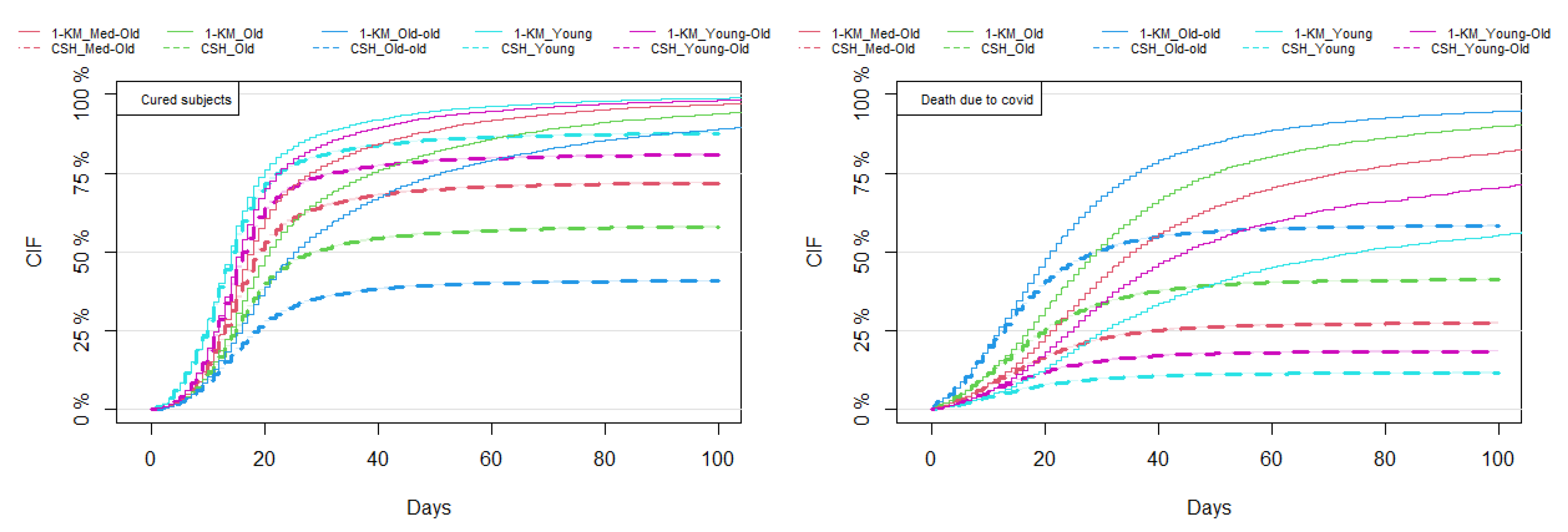
3.2. Results of Non-Parametric Estimation of the CIF

Figure 2 shows the CIFs for cured subjects, death due to COVID-19, and death due to other causes, which were estimated non-parametrically using the Aalen–Johansen estimator. Here, the estimated probability of COVID-19 death was 24 % after the first 20 days from the day of symptoms and became 35 % after 30 days. Meanwhile, the likelihood of becoming cured was 50 % after the first 20 days and around 60 % after 40 days. Death due to other causes was found to be negligible, as the probability of death over time was slightly over zero. This is because, when compared to COVID-19 death and cured subjects, there were very few patients who experienced death due to other causes (only 0.30 % death due to other causes, whereas n = 219 , 325 for COVID-19 death and n = 376 , 549 for cured events, see Figure 1).

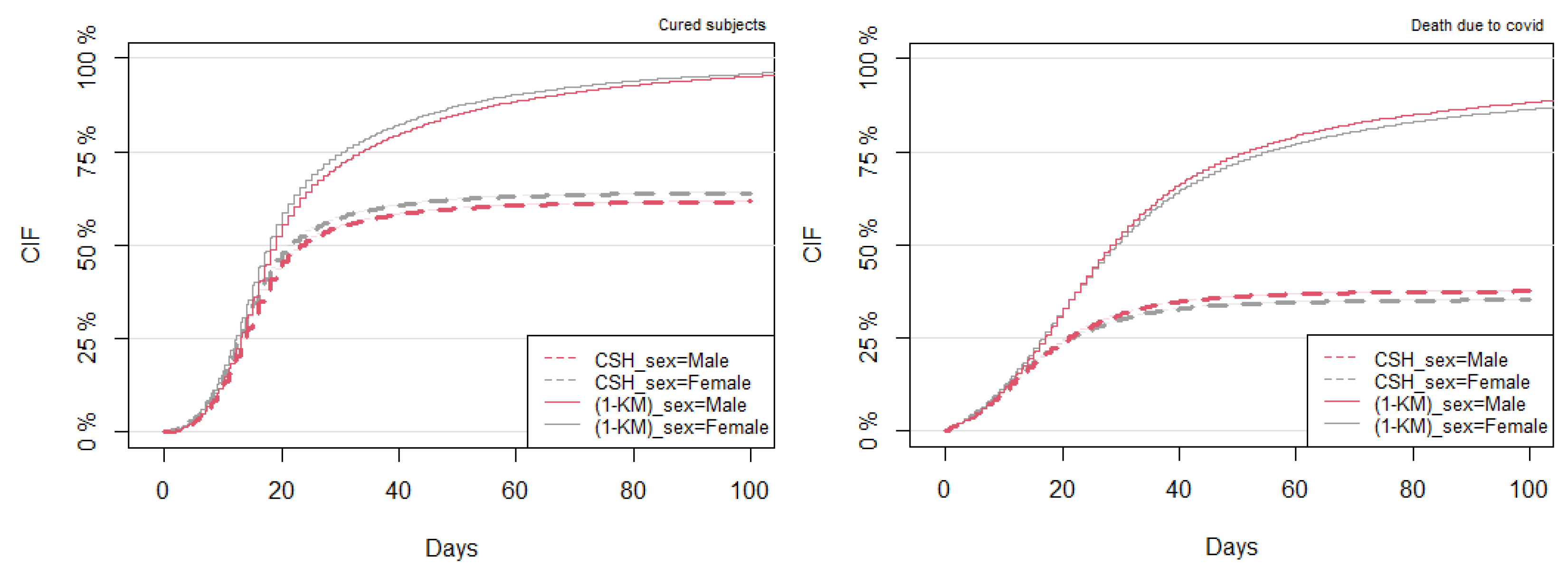
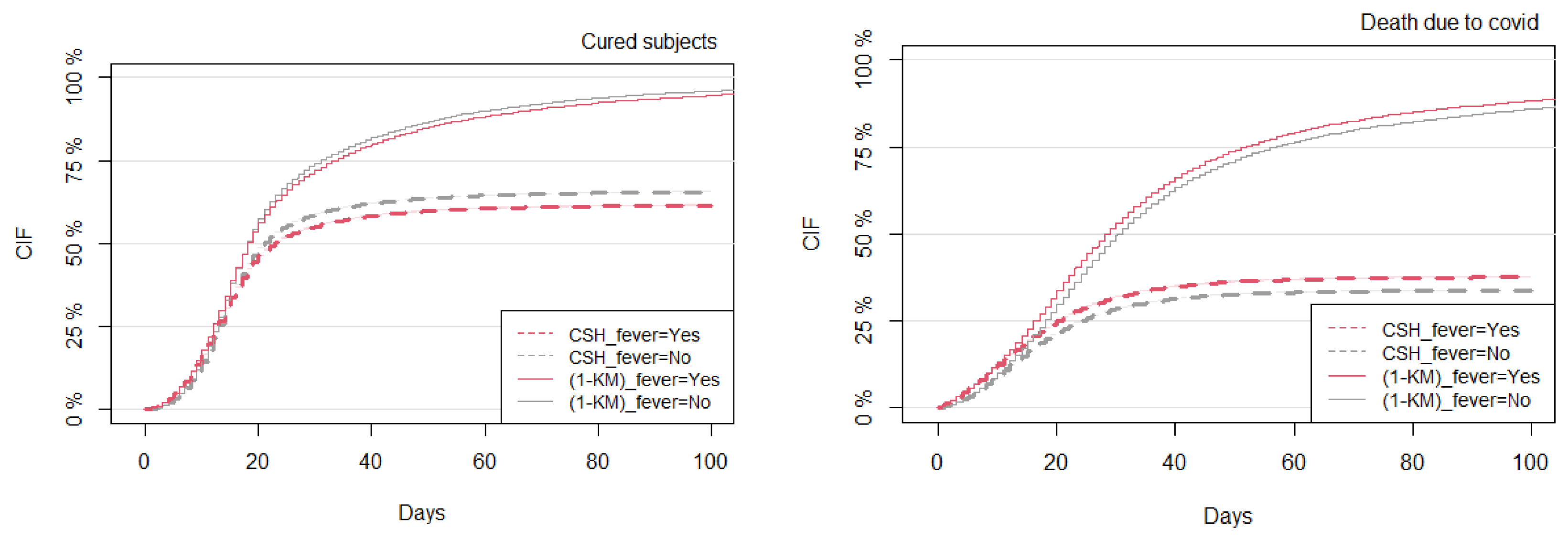
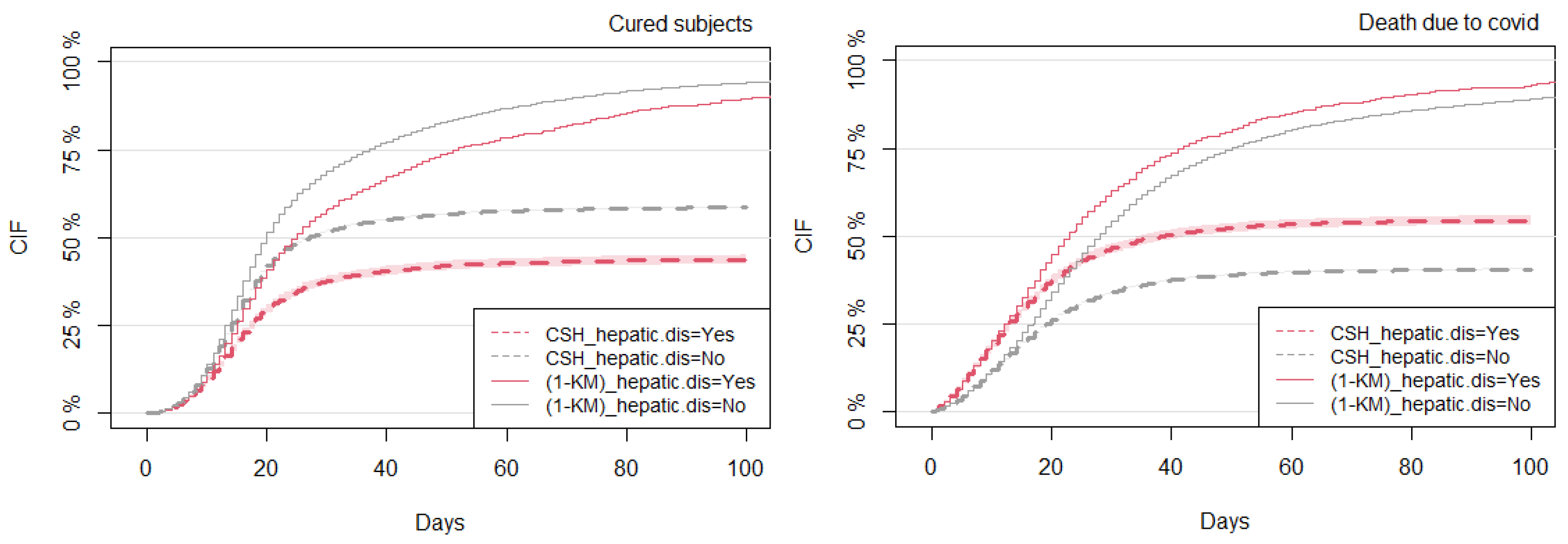
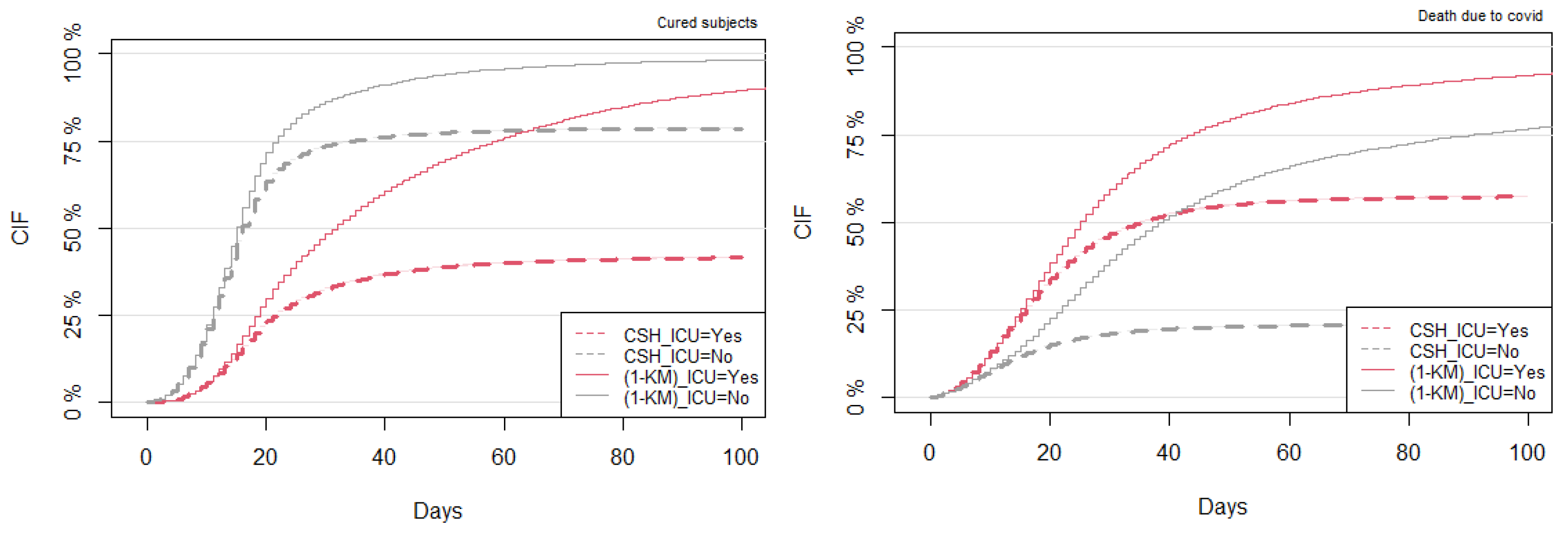
3.3. Comparison between the Kaplan–Meier and CSH Approaches

The objective here was to compute the CIFs based on the conventional technique (K–M) and then compare the results with the competing risks CSH approach. The K–M plot for COVID-19 death estimates the survival probability of subjects who did not experience COVID-19 death. The CIF can be obtained by plotting the complimentary function (1-KM), which estimates the cumulative risk of dying from COVID-19 over time, in the absence of the competing events (here, we treated all of them as right-censored times). Overall, Figure 3, Figure 4, Figure 5, Figure 6, Figure 7, Figure 8, Figure 9, Figure 10, Figure 11 and Figure 12 satisfied the proportional hazards assumption since risk curves do not cross during the analyzed period. A clear overestimation of the CIFs over time was observed under the K–M estimation technique compared with the CSH approach. The overestimation gap between the (1-KM) and CSH approaches was severe, mainly for COVID-19 death. For these reasons, the following results are shown for both the K–M and CSH approaches, but their interpretation is provided only under the CSH approach.
The subjects who developed the exposures of chronic liver disease (hepatic.dis), other symptoms, respiratory discomfort (resp.disc), oxygen saturation level, and ICU admission had a lower probability of survival after 20 days of hospitalization than subjects who did not experience these characteristics. In particular, the most severe exposure group was the one who entered the ICU, and they had about a 40 % less probability of survival after 20 days than those subjects who were not admitted to this unit (Figure 10). Furthermore, the cumulative risk for COVID-19 death was slightly higher among subjects who had a fever, as compared with subjects who did not experience fever (Figure 4). Moreover, the CIFs for subjects who had been vaccinated for the flu and those who had not received the flu vaccine were almost indistinguishable (Figure 5). Additionally, the probability of COVID-19 death for male subjects was higher as compared with female subjects (Figure 3). However, under the CSH approach, flu vaccine and sex exposures were both found to be statistically significant with a hazard ratio of 0.94 and 1.06 , respectively (Table 1). The probability of COVID-19 death increased with older age; in particular, it was more severe for the group with age greater than 70 years, being 50 % after 30 days (‘Old-old’, blue lines in Figure 11). Black subjects were found to have a higher probability of dying from COVID-19 and White subjects were associated with lower risk, as compared with the other races (Figure 12).
Note that, as expected, the results of cured subjects in Figure 3, Figure 4, Figure 5, Figure 6, Figure 7, Figure 8, Figure 9, Figure 10, Figure 11 and Figure 12 show an inverse situation on the CIFs with respect to the curves for COVID-19 death.

3.4. Regression Analysis under the CSH and SDH Approaches

To analyze the effect of the exposures on the CIF, it was found that there were confounding effects among the symptoms and some of the patients’ risk factors. Thus, we separated those confounding exposures and investigated the remaining risk factors on the cause of interest. In particular, the stepwise variable selection techniques were applied based on the AIC and likelihood ratio test under the Cox proportional hazard assumptions for the CSH and SDH approaches. The data were analyzed in R statistical software, version 4.1.1 [24]. The final regression model included the following variables: asthma, diabetes, obesity, other.risk, immuno, kidney, neuro, flu.vaccine, hepatic.dis, age, sex, ICU, pneumo, and race.

3.4.1. Regression Analysis for the CSH Approach

From Table 1, the worst outcome was observed for the age group Old-old (>70 years) with a hazard ratio around two-folds higher (HR: 2.038 , CI: 1.973–2.104) as compared with the reference group of Medium-Old age (50–60 years). Furthermore, subjects who were admitted to the Intensive Cure Unit (ICU) had a significantly higher COVID-19 mortality than those not admitted in the ICU (HR: 1.537 , CI: 1.504–1.571). Moreover, the exposures diabetes, other risks, and male sex had hazard ratios of 1.8 , 1.06 , and 1.06 , respectively, indicating a mortality increase of 6–8% with respect to the their respective reference levels. In addition, it was found that the subjects who had been vaccinated for the flu were associated with a 6 % decreased COVID-19 mortality than those who had not been vaccinated (HR: 0.939 , CI: 0.918–0.960). Moreover, subjects with a state of decreased immunological system function (Immuno), chronic kidney disease, neurological disease, and chronic liver disease (hepatic.dis1) had an increased COVID-19 mortality of approximately 27–31% (HRs = 1.286 , 1.269 , 1.310 , and 1.28 , respectively) as compared with those who had no such disease status. Additionally, the rate of dying due to COVID-19 was significantly higher for all races as compared with White subjects, and, in particular, it was 37 % and 22 % higher, respectively, for Indigenous and Black subjects (HR: 1.370 and CI: 1.136–1.653, HR: 1.219 and CI: 1.165–1.275). Subsequently, the mortality rate for Black and Brown subjects was also found to be significantly higher than that for White subjects. Interestingly, subjects with asthma were found to have a lower COVID-19 mortality (HR: 0.891 , CI: 0.842–0.943) with respect to subjects without this chronic disease. This may be justified by the fact that subjects with asthma were faster hospitalized and received extra care during hospitalization. Thus, the the risk of dying lessened.

3.4.2. Regression Analysis for the SDH Approach

This section explores the performance of the SDH approach, i.e., the Fine–Gray model. This approach makes it possible to obtain both the naive and the robust model-based standard errors. Here, only robust standard errors are reported. It is observed from Table 2 that the estimated coefficients for COVID-19 death deviate slightly from those obtained from the CSH regression model. The differences in the estimated parameters reflect the different underlying assumptions under competing risks survival data. Moreover, note that the CSH model describes the effect on the COVID-19 mortality rate, whereas the Fine–Gray model describes the effect on the cumulative risk of dying from COVID-19, transformed on the scale of the link function. The estimates derived from the Fine–Gray model have no simple interpretation, but they follow the same direction as the CSH model.

3.5. Comparison of Model Predictions between the CSH and SDH Approaches

From the results obtained with the fitted regression models, the model-based predictions can be undertaken and compared by analyzing the subject’s risk with some specific given values for the exposures. As an illustration, let us predict the cumulative risk (CIF) of dying from COVID-19 for subjects with a certain flu vaccination status and chronic liver disease status, under both the CSH and SDH approaches. Figure 13 shows two specific groups based on the two considered subjects’ risk factors: group 1 is related to those who had been vaccinated for the flu and had no chronic liver disease; group 2 refers to those who had not been vaccinated for the flu and had chronic liver disease. From Figure 13 (left panel), it is observed that, at the beginning of the study, the CIF curves between the two groups appear to be similar until day 10. Then, the discrepancy of the CIF probabilities increases over time. In particular, in the CSH approach, the cumulative risk (CIF) of COVID-19 death reaches 50 % in 25 days for group 1, and in 30 days for group 2. Moreover, the CIF probability gap is almost similar from 30 days to more than 100 days. On the contrary, in the SDH approach, after 10 days, the discrepancy in the CIF probabilities between the two groups increased similarly until 25 days, but then later on and up to 70 days, this gap is even more than that under the CSH approach, and finally, after that period, the CIF curves appear to be flat (see Figure 13, right panel).

4. Discussion

We used competing risk survival analyses to estimate the CIF of dying from COVID-19 and the CIF of dying from other causes in subjects with COVID-19 who had been monitored from the time they first showed symptoms to the time they died or left the study because they were cured. In the preliminary stage of this paper (Section 3.2 and Section 3.3), the time to become cured is regarded as one of the events of interest and explored on its own. However, in the later part of this paper, while considering the competing risk settings, this event is considered as censored since the primary focus is on the causes of mortality, in particular on COVID-19 death. This setting goes against the presumption of non-informative censoring. In particular, the likelihood of death among cured patients is not indicative of the likelihood of death among patients remaining hospitalized. Regression models, on the other hand, are particularly pertinent when the techniques are examined using the IPCW technique because they can also take dependent censoring into consideration.
Since the cumulative risk curves did not cross over the studied time, Figure 3, Figure 4, Figure 5, Figure 6, Figure 7, Figure 8, Figure 9, Figure 10, Figure 11 and Figure 12 generally satisfied the proportional hazards assumption. In comparison with the CSH approach, the K–M estimation strategy clearly overestimated the CIF functions over time. A significant overestimation gap was observed between the two approaches, particularly for COVID-19 deaths. The exposures of asthma, diabetes, obesity, other.risk, immuno, kidney, neuro, flu.vaccine, hepatic.dis, age, sex, ICU, pneumo, and race significantly increase the probability of death due to COVID-19. The highest hazard ratio, equal to 2.03 , was observed for subjects with age greater than 70 years compared with the age group 50–60 years. The Fine–Gray model (SDH approach) yielded estimated coefficients for death due to COVID-19 that differed slightly from the CSH model’s results. The disparities in the predicted parameters from the two approaches mirrored the differing underlying model assumptions for the competing risks setting.
Furthermore, from the fitted regression models, model-based predictions were undertaken and evaluated by assessing a certain subject’s risk with the desired specified exposures. In the COVID-19 application, it was found that the SDH approach provides slightly higher estimated Cumulative Incidence Functions as compared with the CSH approach. Nowadays, competing risks data are found in many fields, ranging from medicine, where several types of oncology and therapeutic outcomes are studied simultaneously over time, to epidemiology, demography, and reliability, where, e.g., failure may be due to the breakdown of a mechanical device for several different causes. Therefore, the construction of accurate regression models for competing risks data based on the two discussed approaches (the CSH and SDH methods) is of potentially great interest in many other contexts and applied fields. Furthermore, based on the fitted models, all desired individual predictions of CIFs can be computed on the same data, i.e., the training data, but also on new data, i.e., the testing data, and prediction accuracy can be measured. The competing risks regression models described in this paper provide a very important foundation for obtaining accurate personalized predictions, on which, e.g., many current statistical learning and personalized medicine techniques are based.
In this study, the ICU is considered a time-constant exposure, but more appropriately, one may also consider the ICU as a time-dependent covariate. Moreover, it could also be of interest to study its time-varying effect on the CIFs. Due to the presence of acute severe respiratory failure in a significant proportion of COVID-19 cases, hospitalization, admission to the Intensive Care Unit, and intubation are frequently necessary to treat these cases [25]. Thus, alternative approaches such as extension to multi-state regression models [26] or direct regression models based on binomial regression [27] could help with predicting such an objective, allowing one to model time-dependent covariates and time-varying coefficients. Furthermore, although the estimation technique by [11] is efficient to estimate the proportional SDHs, alternative approaches such as pseudo-value and binomial regression approaches have more flexibility to model the CIF directly through different link functions. Nevertheless, the interpretation of the regression parameters in all these approaches is direct but not straightforward, depending on the chosen link function. However, computation and graphical representation of the CIF curves between different risk factor groups are straightforward and always possible to help one make personalized individual clinical decisions.
The data may not be comprehensive for all of the Brazilian COVID-19 population due to possible errors in the compilation and registration of the information by the diseased patients or the Personnel of the Ministry offices. The registration of cured patients was recorded only on some days and not continuously, providing some possible underestimation of the CIF for cured subjects. In addition, our analyses have the limitation that they do not further investigate the difference in the CIF between subjects who have one or more risk factors from subjects without risk factors, and they do not account for delayed entry into the ICU.

Author Contributions

Conceptualization, M.A.H.; methodology, G.C.; software and data validation, G.C. and M.A.H.; formal analysis, M.A.H.; investigation, G.C.; resources, G.C.; data curation, M.A.H.; original draft preparation, M.A.H.; draft review and editing, G.C.; data visualization, M.A.H.; supervision, G.C.; project administration, G.C.; funding acquisition, G.C. All authors have read and agreed to the published version of the manuscript.

Funding

This research was funded by the Italian Ministry of University and Research (MIUR) with the grant PRIN2017 (20178S4EK9).

Data Availability Statement

The COVID-19 data from 1 January 2020 to 30 April 2021 can be obtained from the Ministry of Health of Brazil.

Acknowledgments

The authors highly acknowledge the University of Padua for administrative and technical support.

Conflicts of Interest

The authors declare no conflict of interest. The funders had no role in the design of the study; in the collection, analyses, or interpretation of data; in the writing of the manuscript; or in the decision to publish the results.

Abbreviations

The following abbreviations are used in this manuscript:
COVID-19Coronavirus Disease-2019
SARS-CoV2Severe Acute Respiratory Syndrome Coronavirus 2
CRsCompeting Risks
CIFCumulative Incidence Function
K–MKaplan–Meier
CSHCause-Specific Hazard
SDHSub-Distribution Hazard
AICAkaike information criterion
ICUIntensive Care Unit
HRHazard Ratio
IPCWInverse of the Probability of Censoring Weights

References

  1. Ge, H.; Wang, X.; Yuan, X.; Xiao, G.; Wang, C.; Deng, T.; Yuan, Q.; Xiao, X. The epidemiology and clinical information about COVID-19. Eur. J. Clin. Microbiol. Infect. Dis. 2020, 39, 1011–1019. [Google Scholar] [CrossRef] [PubMed]
  2. Ghosh, S.; Samanta, G.P.; Mubayi, A. Comparison of regression approaches for analyzing survival data in the presence of competing risks. Lett. Biomath. 2021, 8, 29–47. [Google Scholar]
  3. Zuccaro, V.; Celsa, C.; Sambo, M.; Battaglia, S.; Sacchi, P.; Biscarini, S.; Valsecchi, P.; Pieri, T.C.; Gallazzi, I.; Colaneri, M.; et al. Competing-risk analysis of coronavirus disease 2019 in-hospital mortality in a Northern Italian centre from SMAtteo COVID-19 REgistry (SMACORE). Sci. Rep. 2021, 11, 1137. [Google Scholar] [CrossRef] [PubMed]
  4. Salinas-Escudero, G.; Carrillo-Vega, M.F.; Granados-García, V.; Martínez-Valverde, S.; Toledano-Toledano, F.; Garduño-Espinosa, J. A survival analysis of COVID-19 in the Mexican population. BMC Public Health 2020, 20, 1616. [Google Scholar]
  5. Nijman, G.; Wientjes, M.; Ramjith, J.; Janssen, N.; Hoogerwerf, J.; Abbink, E.; Blaauw, M.; Dofferhoff, T.; van Apeldoorn, M.; Veerman, K.; et al. Risk factors for in-hospital mortality in laboratory-confirmed COVID-19 patients in the Netherlands: A competing risk survival analysis. PLoS ONE 2021, 16, e0249231. [Google Scholar] [CrossRef]
  6. Rathouz, P.J.; Valencia, V.; Chang, P.; Morton, D.; Yang, H.; Surer, O.; Fox, S.; Meyers, L.A.; Matsui, E.C.; Haynes, A.B. Survival analysis methods for analysis of hospitalization data: Application to COVID-19 patient hospitalization experience. medRxiv, 2021; Preprint. [Google Scholar] [CrossRef]
  7. Kim, H.T. Cumulative incidence in competing risks data and competing risks regression analysis. Clin. Cancer Res. 2007, 13, 559–565. [Google Scholar] [CrossRef]
  8. Guo, C.; So, Y. Cause-specific analysis of competing risks using the PHREG procedure. SAS Glob. Forum 2018, 2018, 18. [Google Scholar]
  9. Kaplan, E.L.; Meier, P. Nonparametric estimation from incomplete observations. JASA 1958, 53, 457–481. [Google Scholar] [CrossRef]
  10. Andersen, P.K.; Borgan, Ø.; Gill, R.D.; Keiding, N. Statistical Models Based on Counting Processes; Springer Science & Business Media: Berlin/Heidelberg, Germany, 2012. [Google Scholar]
  11. Fine, J.P.; Gray, R.J. A proportional hazards model for the subdistribution of a competing risk. JASA 1999, 94, 496–509. [Google Scholar] [CrossRef]
  12. Satagopan, J.M.; Ben-Porat, L.; Berwick, M.; Robson, M.; Kutler, D.; Auerbach, A.D. A note on competing risks in survival data analysis. Br. J. Cancer 2004, 9, 1229–1235. [Google Scholar] [CrossRef] [PubMed]
  13. Bender, R.; Augustin, T.; Blettner, M. Generating survival times to simulate Cox proportional hazards models. Stat. Med. 2005, 24, 1713–1723. [Google Scholar] [CrossRef] [PubMed]
  14. Klein, J.P.; Van, H.; Hans, C.; Ibrahim, J.G.; Scheike, T.H. Handbook of Survival Analysis; CRC Press: Boca Raton, FL, USA, 2014. [Google Scholar]
  15. Haller, B. The Analysis of Competing Risks Data with a Focus on Estimation of Cause-Specific and Subdistribution Hazard Ratios from a Mixture Model. Ph.D. Thesis, LMU School, Munchen, Germany, 2014. [Google Scholar]
  16. Aalen, O. Nonparametric inference for a family of counting processes. Ann. Stat. 1978, 6, 701–726. [Google Scholar] [CrossRef]
  17. Aalen, O.O.; Johansen, S. An empirical transition matrix for non-homogeneous Markov chains based on censored observations. Scand. J. Statist. 1978, 5, 141–150. [Google Scholar]
  18. Prentice, R.L.; Kalbfleisch, J.D.; Peterson, A.V., Jr.; Flournoy, N.; Farewell, V.T.; Breslow, N.E. The analysis of failure times in the presence of competing risks. Biometrics 1978, 34, 541–554. [Google Scholar] [CrossRef]
  19. Cheng, S.; Fine, J.P.; Wei, L. Prediction of cumulative incidence function under the proportional hazards model. Biometrics 1998, 54, 219–228. [Google Scholar] [CrossRef]
  20. Bickel, P.J.; Doksum, T. Mathematical Statistics, 2nd ed.; Springer Prentice-Hall: Berlin/Heidelberg, Germany, 2001. [Google Scholar]
  21. Demidenko, E. Mixed Models: Theory and Applications with R; John Wiley & Sons: Hoboken, NJ, USA, 2013. [Google Scholar]
  22. Demidenko, E. Sample size determination for logistic regression revisited. Stat. Med. 2007, 26, 3385–3397. [Google Scholar] [CrossRef]
  23. Gray, R.J. A class of K-sample tests for comparing the cumulative incidence of a competing risk. Ann. Stat. 1988, 16, 1141–1154. [Google Scholar] [CrossRef]
  24. R Core Team: A Language and Environment for Statistical Computing; R Foundation for Statistical Computing: Vienna, Austria, 2019; Available online: Https://www.R-project.org/ (accessed on 19 August 2023).
  25. Lai, C.C.; Shih, T.P.; Ko, W.C.; Tang, H.J.; Hsueh, P.R. Severe acute respiratory syndrome coronavirus 2 (SARS-CoV-2) and coronavirus disease-2019 (COVID-19): The epidemic and the challenges. Int. J. Antimicrob. Agents 2020, 55, 105924. [Google Scholar] [CrossRef]
  26. Cortese, G.; Gerds, T.A.; Andersen, P.K. Comparing predictions among competing risks models with time–Dependent covariates. Stat. Med. 2013, 32, 3089–3101. [Google Scholar] [CrossRef]
  27. Scheike, T.H.; Mei-Jie, Z.; Gerds, T.A. Cumulative Incidence Probability by Direct Binomial Regression. Biometrika 2008, 49, 205–220. [Google Scholar] [CrossRef]
Figure 1. Outcome variable for one main event of interest and two competing events.
Mathematics 11 03772 g001
Figure 2. Cumulative Incidence Functions (CIFs) for subjects who were cured from COVID-19, death due to COVID-19, and other causes of death in the whole population.
Mathematics 11 03772 g002
Figure 3. Cumulative Incidence Function (CIF) curves for exposure sex.
Mathematics 11 03772 g003
Figure 4. Cumulative Incidence Function (CIF) curves for exposure fever.
Mathematics 11 03772 g004
Figure 5. Cumulative Incidence Function (CIF) curves for exposure flu vaccine.
Mathematics 11 03772 g005
Figure 6. Cumulative Incidence Function (CIF) curves for exposure hepatic.dis (chronic liver disease).
Mathematics 11 03772 g006
Figure 7. Cumulative Incidence Function (CIF) curves for exposure other.symp (other symptoms).
Mathematics 11 03772 g007
Figure 8. Cumulative Incidence Function (CIF) curves for exposure resp.disc (respiratory discomfort).
Mathematics 11 03772 g008
Figure 9. Cumulative Incidence Function (CIF) curves for exposure saturation (oxygen saturation).
Mathematics 11 03772 g009
Figure 10. Cumulative Incidence Function (CIF) curves for exposure ICU.
Mathematics 11 03772 g010
Figure 11. Cumulative Incidence Function (CIF) curves for exposure age.
Mathematics 11 03772 g011
Figure 12. Cumulative Incidence Function (CIF) curves for exposure race.
Mathematics 11 03772 g012
Figure 13. Predictions of cumulative risk (CIF) of dying from COVID-19 for subjects with flu vaccine and saturation status under the CSH approach (left panel) and the SDH approach (right panel).
Mathematics 11 03772 g013
Table 1. Results from the CSH model for COVID-19 mortality (COVID-19 death is the main event of interest): regression coefficient estimates (‘Estimates’), hazard ratios (HR), standard errors (SE), 95 % confidence intervals (‘Lower CI’, ‘Upper CI’), p-values.
ExposuresEstimatesHRSELower CIUpper CIp-Value
Asthma (Yes)−0.1150.8910.0290.8420.943<0.001
Diabetes (Yes)0.0771.0800.0111.0581.104<0.001
Obesity (Yes)0.0341.0340.0180.9981.0720.060
Other.risk (Yes)0.0581.0600.0111.0381.082<0.001
Immuno (Yes)0.2521.2860.0241.2271.348<0.001
Kidney (Yes)0.2381.2690.0191.2221.317<0.001
Neuro (Yes)0.2701.3100.0191.2621.360<0.001
Flu.vaccine (Yes)−0.0630.9390.0110.9180.960<0.001
Hepatic.dis (Yes)0.2471.2800.0401.1841.384<0.001
Age: Old (60–70 Years)0.2761.3180.0181.2721.366<0.001
Age: Old-old (>70 Years)0.7122.0380.0171.9732.104<0.001
Age: Young (<40 Years)−0.3330.7170.0310.6750.761<0.001
Age: Young-Old (40–50 Years)−0.1200.8870.0260.8440.933<0.001
Sex (Male)0.0601.0620.0111.0401.085<0.001
ICU (Yes)0.4301.5370.0111.5041.571<0.001
Pneumo (Yes)0.1331.1430.0191.1001.187<0.001
Race: Black0.1981.2190.0231.1651.275<0.001
Race: East Asian0.0641.0660.0490.9681.1740.194
Race: Brown0.1491.1600.0111.1351.187<0.001
Race: Indigenous0.3151.3700.0961.1361.653<0.001
‘Other.risk’ = other risk factors; ‘immuno’ = immunosuppression, which is decreased from immunological system function; ‘kidney’ = chronic kidney disease; ‘neuro’ = neurological diseases; ‘flu.vaccine’ = flu vaccine last campaign; ‘hepatic.dis’ = chronic liver disease; ‘pneumo’ = lung chronic disease; ‘ICU’ = admitted to Intensive Care Unit.
Table 2. Results from the Fine–Gray model (SDH approach) for the cumulative incidence of COVID-19 death (main event of interest): regression coefficient estimates (‘Estimates’), hazard ratios (HR), robust standard errors (Robust SE), 95 % confidence intervals (‘Lower CI’, ‘Upper CI’), p-values.
ExposuresEstimatesHRSELower CIUpper CIp-Value
Asthma (Yes)−0.1150.8910.0290.8420.943<0.001
Diabetes (Yes)0.0781.0810.0111.0581.105<0.001
Obesity (Yes)0.0371.0370.0181.0011.075<0.050
Other.risk (Yes)0.0561.0580.0111.0361.081<0.001
Immuno (Yes)0.2411.2720.0251.2111.338<0.001
Kidney (Yes)0.2351.2650.0211.2161.317<0.001
Neuro (Yes)0.2671.3060.0211.2531.361<0.001
Flu.vaccine (Yes)−0.0620.9400.0110.9190.961<0.001
Hepatic.dis (Yes)0.2441.2760.0441.1711.391<0.001
Age: Old (60–70 Years)0.2781.3210.0171.2771.367<0.001
Age: Old-old (>70 Years)0.7102.0350.0161.9712.101<0.001
Age: Young (<40 Years)−0.3350.7150.0300.6740.759<0.001
Age: Young-Old (40–50 Years)−0.1200.8870.0250.8450.931<0.001
Sex (Male)0.0611.0630.0111.0411.086<0.001
ICU (Yes)0.4341.5430.0111.5101.577<0.001
Pneumo (Yes)0.1321.1410.0201.0971.188<0.001
Race: Black0.1981.2190.0241.1641.277<0.001
Race3: East Asian0.0531.0540.0470.9611.1570.264
Race4: Brown0.1441.1550.0121.1291.181<0.001
Race: Indigenous0.3231.3810.1061.1211.701<0.003
‘Other.risk’ = other risk factors; ‘immuno’ = immunosuppression, which is decreased from immunological system function; ‘kidney’ = chronic kidney disease; ‘neuro’ = neurological diseases; ‘flu.vaccine’ = flu vaccine last campaign; ‘hepatic.dis’ = chronic liver disease; ‘pneumo’ = lung chronic disease; ‘ICU’ = admitted to Intensive Care Unit.
Disclaimer/Publisher’s Note: The statements, opinions and data contained in all publications are solely those of the individual author(s) and contributor(s) and not of MDPI and/or the editor(s). MDPI and/or the editor(s) disclaim responsibility for any injury to people or property resulting from any ideas, methods, instructions or products referred to in the content.

