Statistical Inference and Optimal Design of Accelerated Life Testing for the Chen Distribution under Progressive Type-II Censoring

Abstract

This paper discusses statistical inference and optimal design of constant-stress accelerated life testing for the Chen distribution under progressive Type-II censoring. The scale parameter of the life distribution is assumed to be a logarithmic linear function of the stress level. The maximum likelihood estimates of the parameters are obtained. Then, the observed Fisher information matrix is derived and utilized to construct asymptotic confidence intervals. Meanwhile, the parametric bootstrap methods are provided for the interval estimation. In addition, the Bayes estimates under the squared error loss function are obtained by applying the Tierney and Kadane technique and Lindley’s approximation. As for the optimal design, D- and A-optimality criteria are considered to determine the optimal transformed stress level. Finally, the simulation is carried out to demonstrate the proposed estimation techniques and the optimal criteria, and a real data set is discussed.

1. Introduction

In factory production, life testing is of great significance to evaluate product quality. Conventional life testing is to mainly observe the failure time information of all test units under normal usage in order to reveal the life characteristics. However, products are produced more and more reliably currently, so it is difficult or even impossible for them to fail under normal usage. To reduce the cost and time, it is necessary to make the test units fail more quickly. A common way is to perform life testing at higher stress levels than normal, which is called accelerated life testing (ALT). Then, the failure time information obtained is analyzed to extrapolate the life characteristics under the normal stress level. One type of classifying ALT is the way stress changes with time. ALTs are mainly classified into constant-stress ALT (CSALT), step-stress ALT (SSALT) and progressive-stress ALT (PSALT). The different focus of the three types is the relationship between stress loading and testing time. For CSALT, the stress is fixed with time; for SSALT, the stress is increased step by step at specific moments; for PSALT, stress is increased continuously with time. Another type of classifying ALTs is by the number of stress levels. They are mainly divided into simple ALT and multiple ALT. The simple ALT has only two stress levels while the multiple ALT has more than two stress levels.

Some of the earlier works on ALT are mainly based on McCool [1], Nelson [2] and Miller and Nelson [3]. Gradually, the study of ALT has attracted the interest of more and more researchers. For the studies of CSALT, Ismail [4] discussed the estimation of parameters of Weibull distribution in the constant-stress partial ALT under hybrid censoring. Statistical inferences on the acceleration factor and the distribution parameters were made utilizing maximum likelihood and percentile bootstrap. Mohie EI-Din et al. [5] derived the optimal plans for k-level CSALT for Lindley failure data and compared the optimal plans calculated by two optimal criteria with the traditional plan calculated by the asymptotic variance of maximum likelihood estimation. In addition, many researchers studied SSALT. Mohie El-Din et al. [6] explored parametric inference for the extension of exponential distribution on SSALT under progressive Type-II censoring. They assumed the cumulative exposure model and obtained the point estimates and interval estimates such as Bayes estimation and parametric bootstrap intervals. Chandra and Khan [7] studied the optimum test plan and parameter estimation for a Lomax distribution for 3-step SSALT under modified progressive Type-I censoring. Interval and point estimates of the model parameters were obtained, and the Bayes estimates are obtained based on Gibbs sampling. Regarding the studies of PSALT, Abdel-Hamid and Abushal [8] applied PSALT when the product lifetime under design stress followed the exponential distribution. Bayes estimates were obtained and compared with maximum likelihood estimates.

Obtaining complete failure time data is ideal in life testing. However, considering the time cost and the possibility of unexpected product failure in practice, researchers increasingly focus on the application of the censoring method. The two basic censoring methods are Type-I and Type-II censoring. A life test is terminated at a fixed time and the surviving test units are withdrawn in Type-I censoring, whereas a life test is terminated when a specified number of units fail in Type-II censoring. Considering that the surviving units can only be withdrawn at the final termination point of the life test, progressive censoring has been more and more popular which enables to withdraw units at various points in the life test. For example, the progressive Type-II censoring is commonly applied in various fields. For more studies on progressive censoring, one can refer to Balakrishnan and Aggarwala [9] and Balakrishnan [10]. Jaheen et al. [11] investigated Bayes inference of constant-partial ALT when the lifetime of test units follows the generalized exponential distribution. Under progressive Type-II censoring, the maximum likelihood and Bayes methods of estimation were utilized for estimating acceleration factor and parameters. Basak and Balakrishnan [12] discussed the problem of predicting survival times of units for the exponential distribution in the simple step-stress testing under progressive Type-II censoring. The maximum likelihood predictors and the conditional median predictors were derived. Abd El-Raheem [13] considered optimal design and estimation of multiple CSALT for generalized half-normal distribution under progressive Type-II censoring. Using various estimation methods, point estimation, interval estimation and predictive estimation were obtained and the optimal transformed stress level was derived using the optimal criteria. Algarni et al. [14] considered E-Bayesian estimation of the scale parameter, hazard and reliability rate functions of the Chen distribution under Type-I censoring. On the basis of the balanced squared error loss function, the gamma distribution was used as a conjugate prior for the scale parameter and three different distributions were discussed for the hyper-parameters.

Chen [15] proposed a two-parameter lifetime distribution with an increasing or bathtub-shaped hazard function. It has been considered by many researchers because the bathtub-shaped hazard function is a suitable conceptual model for a number of machinery and electronics; see Hjorth [16] and Olkin [17]. Due to the various good properties of the Chen distribution, many authors have discussed its statistical inference. Sarhan et al. [18] obtained the Bayes estimation of parameters with gamma priors for the Chen distribution by different approximations methods and compared the maximum likelihood estimates with the approximate Bayesian estimates under non-informative prior. Rastogi and Tripathi [19] used hybrid censoring to estimate unknown parameters of the Chen distribution. Maximum likelihood estimates were obtained by the EM algorithm and Bayes estimates were evaluated by the Tierney and Kadane method and Lindley method. Asymptotic and parametric bootstrap intervals were also proposed. Ahmed [20] derived the Bayes estimators of the parameters, reliability, and hazard function for the Chen distribution under both the balanced linear-exponential loss and balanced-squared error loss utilizing the MCMC method. Moreover, to construct the asymptotic confidence intervals, delta and parametric bootstrap methods were applied to find the variance.

Considering that ALT is relatively rarely used for the Chen distribution which has a bathtub-shaped hazard function and that optimal design studies are less concerned with solving for optimal transformed stress levels, we apply the CSALT model to test units whose lifetimes follow the Chen distribution in the presence of progressive Type-II censoring in this paper. To better estimate the lifetime characteristics of products, we discuss a variety of parameter and interval estimation methods. The maximum likelihood estimates of the parameters for the Chen distribution are obtained under progressive censoring. The Bayes estimates of the parameters are derived by both the Tierney and Kadane technique and Lindley’s approximation. We also discuss three types of confidence intervals which are the asymptotic confidence interval, the bootstrap percentile confidence interval, and the bootstrap-t confidence interval. In addition, to better estimate the life parameters of products under the normal stress level, two optimal criteria are utilized to determine and specify the optimal transformed stress level of CSALT. To measure the performance of the estimates, we conduct some simulations.

The rest of this paper is organized as follows. In Section 2, we discussed some properties of the Chen distribution. In Section 3, we propose the progressive censoring scheme and necessary model assumptions. Then, the maximum likelihood estimates are obtained in Section 4. In Section 5, we derive the Fisher information matrix and the variance–covariance matrix. The asymptotic confidence intervals are also constructed. In Section 6, we present the parametric bootstrap confidence intervals. In Section 7, we discuss the Bayesian estimation and utilize the Tierney and Kadane technique and Lindley’s approximation to obtain the approximate estimates. In Section 8, we apply two optimal criteria to determine the optimal transformed stress levels. In Section 9, a numerical study is conducted to illustrate the methods proposed and examine their performance. In addition, a real data set is discussed in Section 10. Finally, we make conclusions.

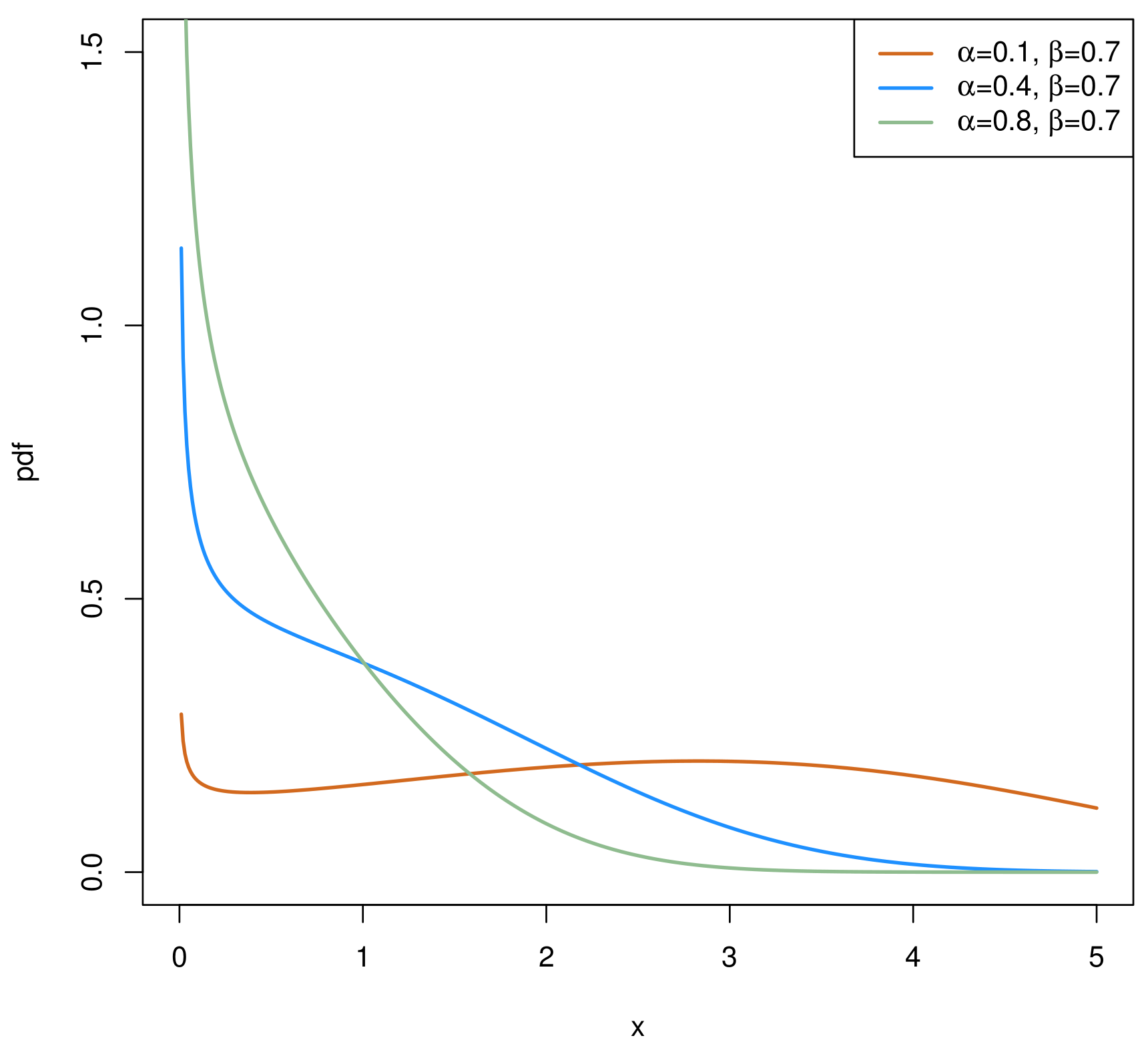
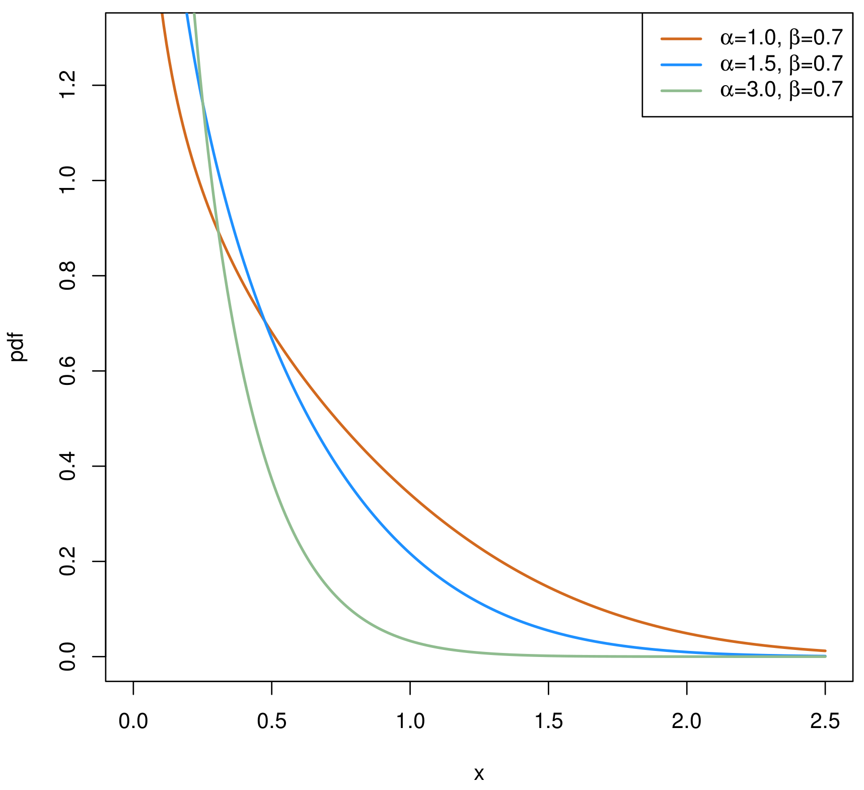
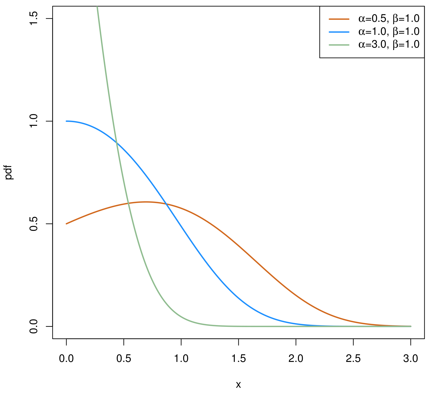
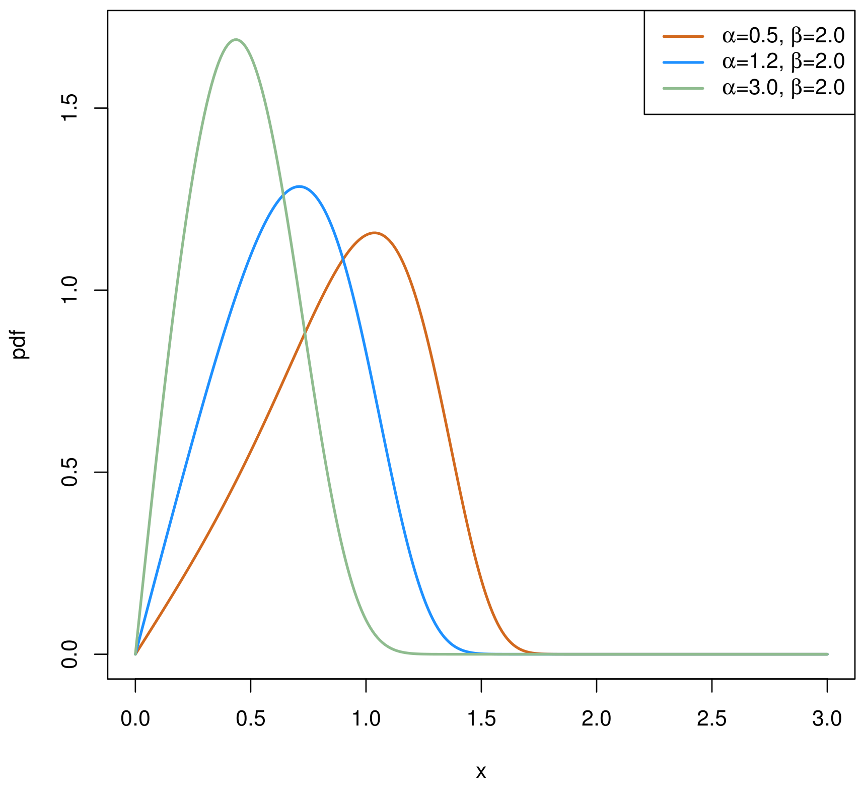
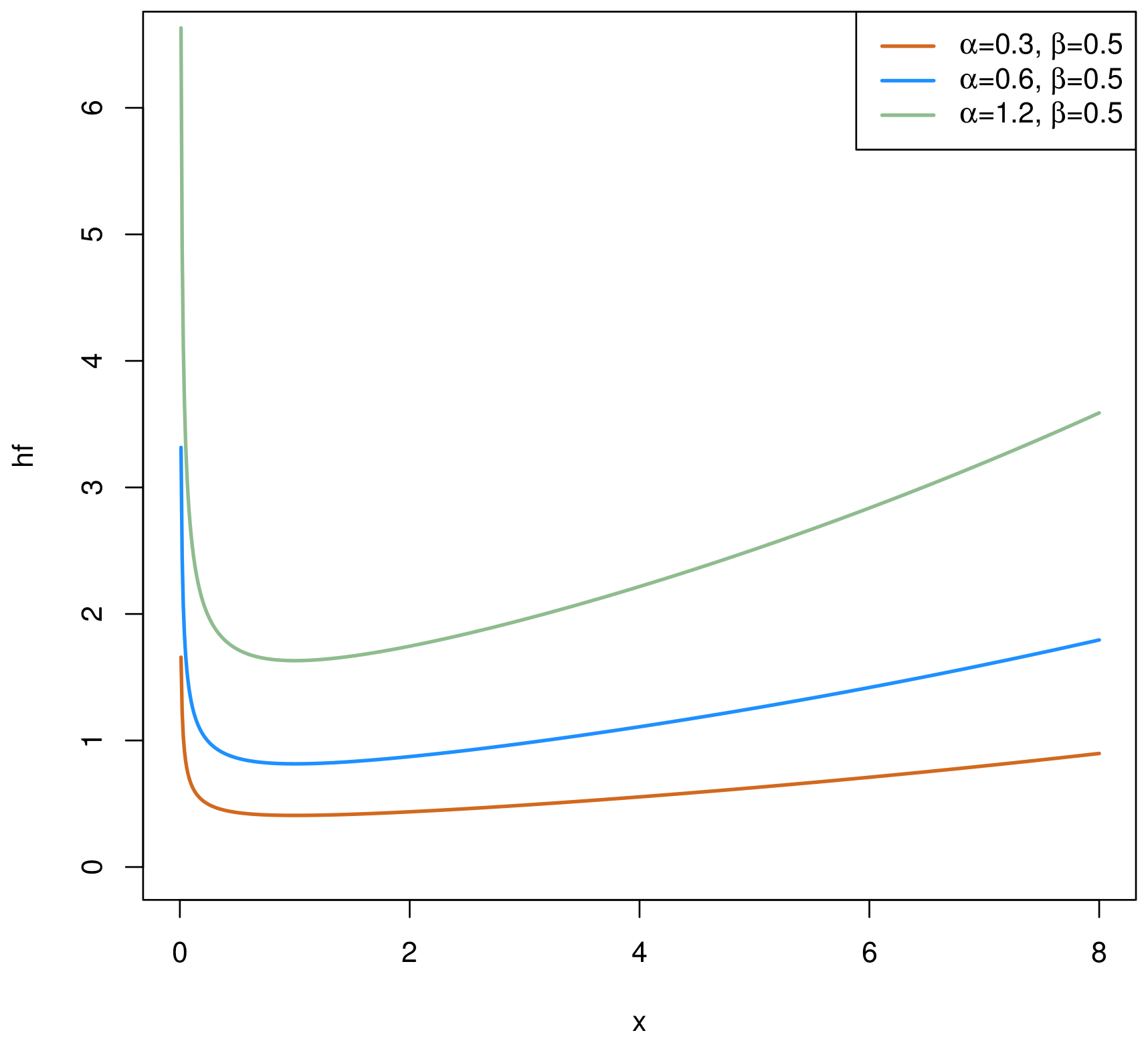
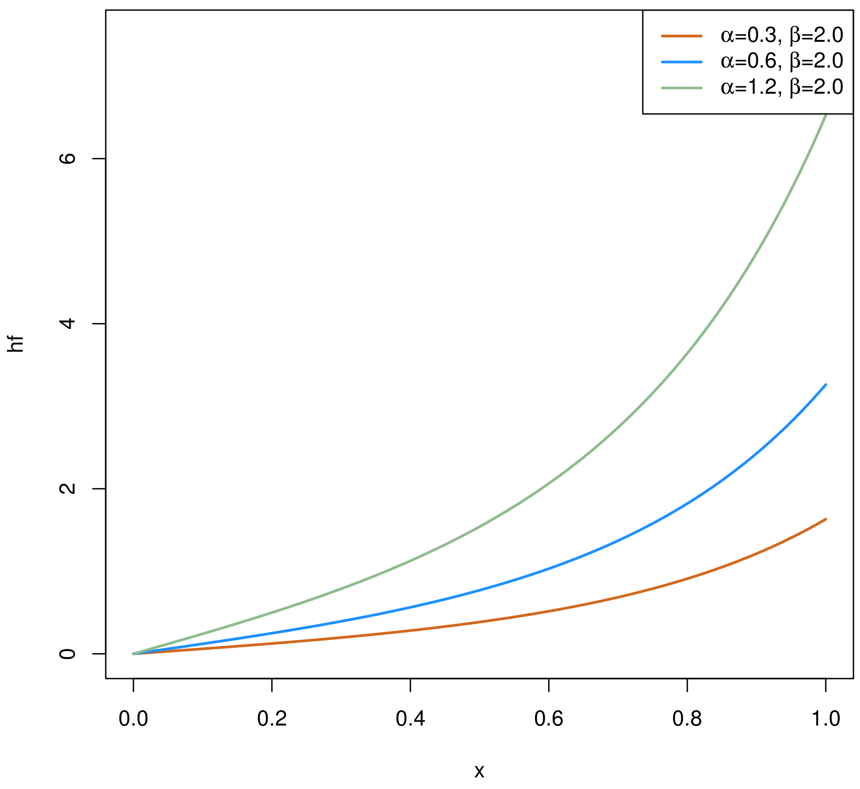
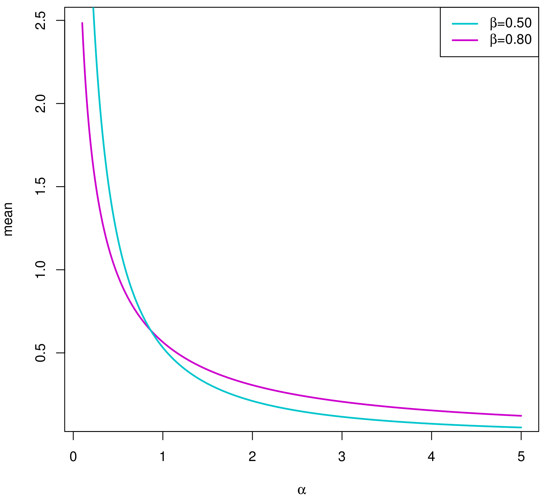
2. The Chen Distribution

The probability density function (pdf), the cumulative distribution function (cdf), and the hazard function (hf) for the Chen distribution are expressed respectively as follows:

$$\begin{array}{c}\hfill f\left(x;\alpha ,\beta \right)=\alpha \beta x^{\beta -1}exp\left\{\alpha \left(1-e^{x^{\beta }}\right)+x^{\beta }\right\},x>0,\alpha >0,\beta >0,\end{array}$$

(1)

$$\begin{array}{c}\hfill F\left(x;\alpha ,\beta \right)=1-exp\left\{\alpha \left(1-e^{x^{\beta }}\right)\right\},x>0,\alpha >0,\beta >0,\end{array}$$

(2)

$$\begin{array}{c}\hfill h\left(x;\alpha ,\beta \right)=\frac{f\left(x;\alpha ,\beta \right)}{1-F\left(x;\alpha ,\beta \right)}=\alpha \beta x^{\beta -1}{e}^{x^{\beta }},x>0,\alpha >0,\beta >0,\end{array}$$

(3)

where $\alpha$ is the scale parameter and $\beta$ is the shape parameter. When $\beta$ is less than one, the hazard function has a bathtub shape, while the shape is increasing when $\beta \ge 1$. Different plots of pdf and hf are shown in Figure 1, Figure 2, Figure 3, Figure 4, Figure 5 and Figure 6. The shape of pdf or hf varies for different parameter values. Assume that $\beta$ is fixed. If $0<\beta <1$: when $0<\alpha <1$, pdf is monotonically decreasing or decreasing, then increasing and finally decreasing, and the tail is thinner with a larger value of $\alpha$; when $\alpha \ge 1$, pdf is monotonically decreasing, and the decrease is sharper with a larger value of $\alpha$. If $\beta =1$: when $0<\alpha <1$, the pdf is unimodal; when $\alpha \ge 1$, the pdf is monotonically decreasing and the decrease is sharper with a larger value of $\alpha$. If $\beta >1$: the pdf is unimodal no matter what $\alpha$ value is taken, and the peak value is larger with a larger value of $\alpha$. From Figure 5 and Figure 6, it can be seen that the hazard rate is larger with a larger value of $\alpha$ if $0<\beta <1$; the rising rate of hf is higher with a larger value of $\alpha$ if $\beta \ge 1$.

When $\beta$ is fixed at some value less than 1, the relationship between the mean of the Chen distribution and $\alpha$ is shown in Figure 7. The mean decreases when the value of $\alpha$ increases. Additionally, letting the cdf of the Chen distribution equal $\frac{1}{2}$, we can solve for the median $x_m={\left[ln\left(1+\frac{1}{\alpha }ln2\right)\right]}^{\frac{1}{\beta }}$. Similarly, when $\beta$ is fixed and $\alpha$ increases, the median decreases.

In addition, the Chen distribution has a great deal of flexibility. Let X be a nonnegative random variable and follow the Chen distribution. Following Ahmed et al. [21], $Y=e^{X^{\beta }}-1$ follows the exponential distribution and $Y={\left(e^{X^{\beta }}-1\right)}^{\frac{1}{\theta }}$ follows the Weibull distribution. Furthermore, the Chen distribution reduces to Gompertz distribution when $\beta =1$.

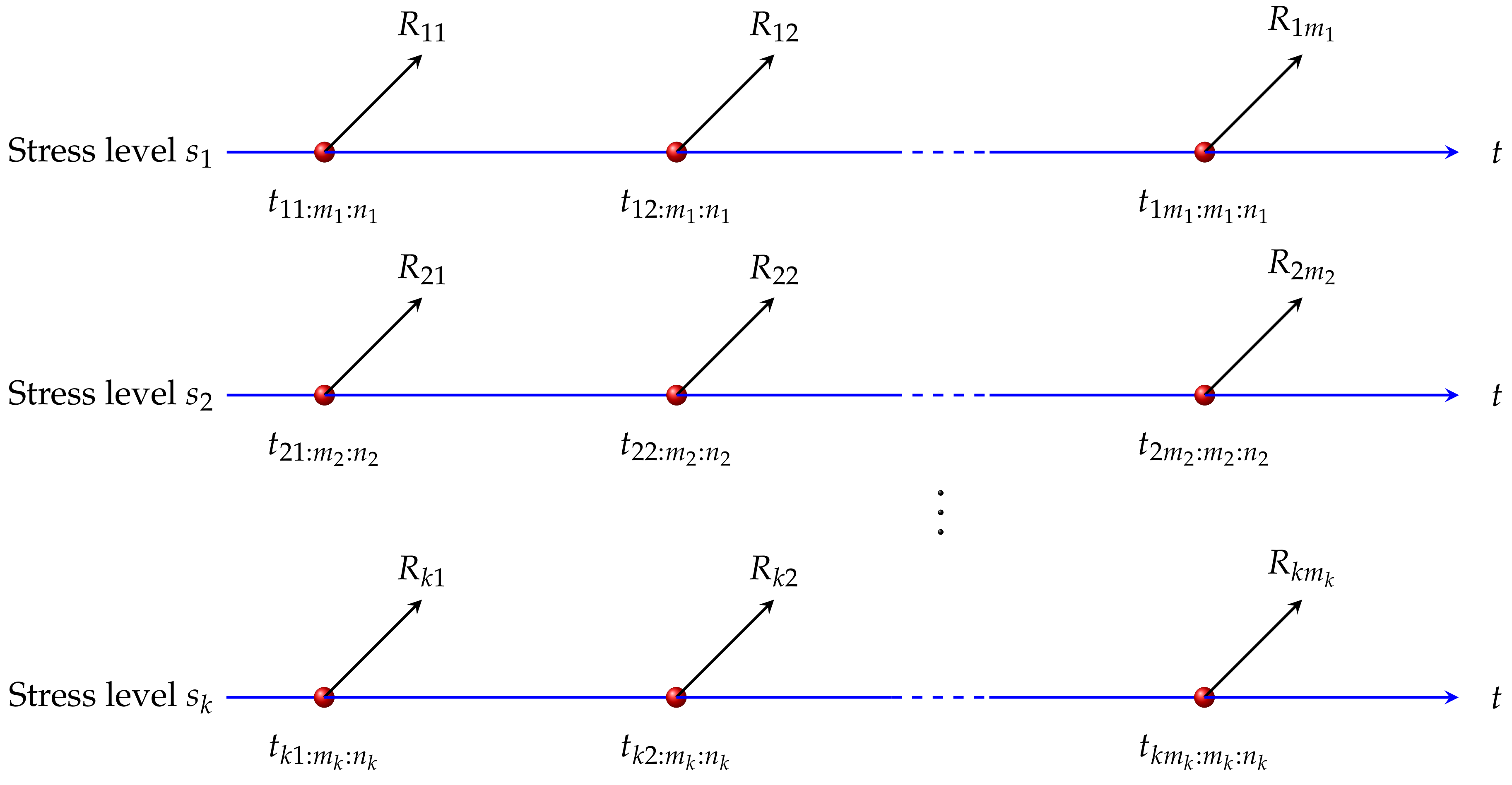
3. Model Assumptions

For CSALT, assume a total of n units under the test and $k\ge 2$ stress levels, $s_1<\cdots <s_k$. At each stress level $s_i$, $i=1,2,\cdots ,k$, $n_i$ identical units are assigned for the test, such that ${\sum }_{i=1}^k{n}_i=n$. The lifetime of each unit $X_{ij}$, $j=1,2,\cdots ,n_i$, follows the Chen distribution. $s_0$ is the normal stress level. The progressive Type-II censoring scheme in CSALT is briefly described as follows: For $i=1,2,\cdots ,k$, when the first failure occurs at time $t_{i1:m_i:n_i}$, $R_{i1}$ units are randomly withdrawn from the remaining $n_i-1$ units whose lifetime $X_{ij}>t_{i1:m_i:n_i}$. Then, when the second failure occurs at time $t_{i2:m_i:n_i}$, $R_{i2}$ units are randomly withdrawn from the remaining $n_i-2-R_{i1}$ units whose lifetime $X_{ij}>t_{i2:m_i:n_i}$. Similarly, when the $m_i$-th $\left(1\le m_i\le n_i\right)$ failure occurs at a random time of $t_{i{m}_i:m_i:n_i}$, all remaining $R_{i{m}_i}=n_i-m_i-{\sum }_{j=1}^{m_i-1}{R}_{ij}$ units are withdrawn and the test is terminated. The censoring scheme is shown in Figure 8. Under stress level $s_i$, $i=1,2,\cdots k$, $\left(R_{i1},R_{i2},\cdots ,R_{i{m}_i}\right)$ is the progressive censoring scheme and $t_{ij:m_i:n_i}$ is the observed progressive censored data that $t_{i1:m_i:n_i}<\cdots <t_{i{m}_i:m_i:n_i}$. Obviously, the sample is complete when $\left(R_{i1},R_{i2},\cdots ,R_{i{m}_i}\right)=\left(0,0,\cdots ,0\right)$ and the sample is Type-II censored when $\left(R_{i1},R_{i2},\cdots ,R_{i{m}_i}\right)=\left(0,\cdots ,0,n_i-m_i\right)$.

The following model assumptions are used throughout the whole paper:

(1)

Under stress level $s_i$, $i=1,2,\cdots ,k$, the lifetimes of the units follow

$$\begin{array}{c}\hfill f_i\left(x;{\alpha }_i,\beta \right)={\alpha }_i\beta x^{\beta -1}exp\left\{{\alpha }_i\left(1-e^{x^{\beta }}\right)+x^{\beta }\right\},x>0,{\alpha }_i>0,\beta >0.\end{array}$$

(4)

(2)

The relationship between the stress level $s_i$ and the lifetime distribution parameter ${\alpha }_i$ is

$$\begin{array}{c}\hfill ln\left({\alpha }_i\right)=b_0+b{\phi }_i,i=0,1,\cdots ,k,\end{array}$$

(5)

where ${\phi }_i=\phi \left(s_i\right)$ is an incremental function of $s_i$. $b_0$ and $b>0$ are unknown parameters.

To simplify the expression, according to the model (5), the scale parameter ${\alpha }_i$ can be presented as

$$\begin{array}{c}\hfill {\alpha }_i={\alpha }_{0}exp\left\{b\left({\phi }_i-{\phi }_0\right)\right\}={\alpha }_0{\lambda }^{h_i},i=0,1,\cdots ,k,\end{array}$$

(6)

where ${\alpha }_0$ is the scale parameter for the Chen distribution under normal stress level $s_0$, ${\phi }_0=\phi \left(s_0\right)$, $\lambda =exp\left\{b\left({\phi }_1-{\phi }_0\right)\right\}=\frac{{\alpha }_1}{{\alpha }_0}>1$ and

$$h_i=\frac{{\phi }_i-{\phi }_0}{{\phi }_1-{\phi }_0},i=1,2,\cdots ,k,$$

which satisfy $h_k>h_{k-1}>\cdots >h_1=1$. Since the Jacobian determinant from $\left(b_0,b,\beta \right)$ to $\left({\alpha }_0,\lambda ,\beta \right)$ is $1/\lambda {\alpha }_0\left({\phi }_1-{\phi }_0\right)>0$, the transformation from the model parameter $\left(b_0,b,\beta \right)$ to $\left({\alpha }_0,\lambda ,\beta \right)$ is mapped one-to-one.

4. Maximum Likelihood Estimation

Based on the above assumptions and notations, when the stress level is $s_i$, the likelihood function of parameters ${\alpha }_0,\lambda$ and $\beta$ is given by

$$\begin{array}{c}\hfill L_i\left({\alpha }_0,\lambda ,\beta \right)=C_i\prod _{j=1}^{m_i}{\alpha }_i\beta t_{ij}^{\beta -1}exp\left\{{\alpha }_i\left(1-e^{t_{ij}^{\beta }}\right)+t_{ij}^{\beta }\right\}{\left(exp\left[{\alpha }_i\left(1-e^{t_{ij}^{\beta }}\right)\right]\right)}^{R_{ij}},\end{array}$$

(7)

where $C_i=n_i\left(n_i-1-R_{i1}\right)\cdots \left(n_i-m_i+1-{\sum }_{j=1}^{m_i-1}{R}_{ij}\right)$ and $t_{ij}=t_{ij:m_i:n_i}$. Then, the likelihood function is given by

$$\begin{array}{ccc}\hfill L\left({\alpha }_0,\lambda ,\beta \right)& =& \prod _{i=1}^k{L}_i\left({\alpha }_0,\lambda ,\beta \right)\hfill \\ & & =\prod _{i=1}^k{C}_i\prod _{j=1}^{m_i}{\alpha }_i\beta t_{ij}^{\beta -1}exp\left\{{\alpha }_i\left(1-e^{t_{ij}^{\beta }}\right)+t_{ij}^{\beta }\right\}{\left(exp\left[{\alpha }_i\left(1-e^{t_{ij}^{\beta }}\right)\right]\right)}^{R_{ij}}.\hfill \end{array}$$

(8)

Correspondingly, the log-likelihood function ignoring the constants is given by

$$\begin{array}{ccc}\hfill l\left({\alpha }_0,\lambda ,\beta \right)& =& lnL\left({\alpha }_0,\lambda ,\beta \right)=ln\left(\beta \right){\sum }_{i=1}^k{m}_i+{\sum }_{i=1}^k{m}_{i}ln\left({\alpha }_i\right)+\left(\beta -1\right){\sum }_{i=1}^k{\sum }_{j=1}^{m_i}ln\left(t_{ij}\right)\hfill \\ & & +{\sum }_{i=1}^k{\sum }_{j=1}^{m_i}{\alpha }_i\left(R_{ij}+1\right)\left(1-e^{t_{ij}^{\beta }}\right)+{\sum }_{i=1}^k{\sum }_{j=1}^{m_i}{t}_{ij}^{\beta }.\hfill \end{array}$$

(9)

The partial derivatives of $l\left({\alpha }_0,\lambda ,\beta \right)$ with respect to ${\alpha }_0,\lambda$ and $\beta$ are given by

$$\begin{array}{c}\hfill \frac{\partial l}{\partial {\alpha }_0}=\frac{1}{{\alpha }_0}{\sum }_{i=1}^k{m}_i+{\sum }_{i=1}^k{\sum }_{j=1}^{m_i}{\lambda }^{h_i}\left(R_{ij}+1\right)\left(1-e^{t_{ij}^{\beta }}\right),\end{array}$$

(10)

$$\begin{array}{c}\hfill \frac{\partial l}{\partial \lambda }=\frac{1}{\lambda }{\sum }_{i=1}^k{m}_i{h}_i+{\sum }_{i=1}^k{\sum }_{j=1}^{m_i}{\alpha }_0{h}_i{\lambda }^{h_i-1}\left(R_{ij}+1\right)\left(1-e^{t_{ij}^{\beta }}\right),\end{array}$$

(11)

$$\begin{array}{c}\hfill \frac{\partial l}{\partial \beta }=\frac{1}{\beta }{\sum }_{i=1}^k{m}_i+{\sum }_{i=1}^k{\sum }_{j=1}^{m_i}\left(t_{ij}^{\beta }+1\right)ln\left(t_{ij}\right)-{\sum }_{i=1}^k{\sum }_{j=1}^{m_i}{\alpha }_i{e}^{t_{ij}^{\beta }}{t}_{ij}^{\beta }ln\left(t_{ij}\right)\left(R_{ij}+1\right).\end{array}$$

(12)

We can solve the maximum likelihood estimates (MLE) $\left({\hat{\alpha }}_0,\hat{\lambda },\hat{\beta }\right)$ for ${\alpha }_0,\lambda$ and $\beta$ by making the functions (10)–(12) equal to 0 simultaneously. Unfortunately, explicit solutions cannot be obtained and numerical methods such as the Newton–Raphson method can be utilized to calculate the estimates. According to MacDonald [22], for a constrained optimization problem, one can enforce the constraint by means of a transformation or use of a constrained optimizer. Considering the three parameters are constrained ($\alpha >0$, $\lambda >1$, $\beta >0$), we use the optim function in R software with method L-BFGS-B and default settings. L-BFGS-B is an application of the quasi-Newton method.

5. Fisher Information Matrix

Let $\mathrm{\Theta }=\left({\alpha }_0,\lambda ,\beta \right)$ and T be the observed failure data. For a large-size sample, the inverse of the Fisher information matrix (FIM) can be regarded as the approximation of the variance–covariance matrix. First, FIM is given as follows by evaluating the negative of the expected values of the second-order derivatives and mixed partial derivatives of log-likelihood function in (9) with respect to ${\alpha }_0$, $\lambda$ and $\beta$,

$$\begin{array}{c}\hfill I_T\left(\mathrm{\Theta }\right)=E\left(-\frac{{\partial }^{2}l\left(\mathrm{\Theta }\right)}{\partial {\mathrm{\Theta }}^2}\right)=\left[\begin{array}{ccc}E\left(-\frac{{\partial }^{2}l\left(\mathrm{\Theta }\right)}{\partial {\alpha }_0^2}\right)& E\left(-\frac{{\partial }^{2}l\left(\mathrm{\Theta }\right)}{\partial {\alpha }_0\partial \lambda }\right)& E\left(-\frac{{\partial }^{2}l\left(\mathrm{\Theta }\right)}{\partial {\alpha }_0\partial \beta }\right)\\ E\left(-\frac{{\partial }^{2}l\left(\mathrm{\Theta }\right)}{\partial \lambda \partial {\alpha }_0}\right)& E\left(-\frac{{\partial }^{2}l\left(\mathrm{\Theta }\right)}{\partial {\lambda }^2}\right)& E\left(-\frac{{\partial }^{2}l\left(\mathrm{\Theta }\right)}{\partial \lambda \partial \beta }\right)\\ E\left(-\frac{{\partial }^{2}l\left(\mathrm{\Theta }\right)}{\partial \beta \partial {\alpha }_0}\right)& E\left(-\frac{{\partial }^{2}l\left(\mathrm{\Theta }\right)}{\partial \beta \partial \lambda }\right)& E\left(-\frac{{\partial }^{2}l\left(\mathrm{\Theta }\right)}{\partial {\beta }^2}\right)\end{array}\right].\end{array}$$

(13)

Due to the complexity of the pdf and the integral formula, in practice, the observed FIM which utilizes the MLEs of parameters $\hat{\mathrm{\Theta }}=\left({\hat{\alpha }}_0,\hat{\lambda },\hat{\beta }\right)$ is used to approximate the exact values,

$$\begin{array}{c}\hfill O_T\left(\mathrm{\Theta }\right)={\left[\begin{array}{ccc}-\frac{{\partial }^{2}l\left(\mathrm{\Theta }\right)}{\partial {\alpha }_0^2}& -\frac{{\partial }^{2}l\left(\mathrm{\Theta }\right)}{\partial {\alpha }_0\partial \lambda }& -\frac{{\partial }^{2}l\left(\mathrm{\Theta }\right)}{\partial {\alpha }_0\partial \beta }\\ -\frac{{\partial }^{2}l\left(\mathrm{\Theta }\right)}{\partial \lambda \partial {\alpha }_0}& -\frac{{\partial }^{2}l\left(\mathrm{\Theta }\right)}{\partial {\lambda }^2}& -\frac{{\partial }^{2}l\left(\mathrm{\Theta }\right)}{\partial \lambda \partial \beta }\\ -\frac{{\partial }^{2}l\left(\mathrm{\Theta }\right)}{\partial \beta \partial {\alpha }_0}& -\frac{{\partial }^{2}l\left(\mathrm{\Theta }\right)}{\partial \beta \partial \lambda }& -\frac{{\partial }^{2}l\left(\mathrm{\Theta }\right)}{\partial {\beta }^2}\end{array}\right]}_{\mid {\alpha }_0={\hat{\alpha }}_0,\lambda =\hat{\lambda },\beta =\hat{\beta }},\end{array}$$

(14)

where

$$\begin{array}{c}\hfill -\frac{{\partial }^{2}l\left(\mathrm{\Theta }\right)}{\partial {\alpha }_0^2}=\frac{{\sum }_{i=1}^k{m}_i}{{\alpha }_0^2},\end{array}$$

(15)

$$\begin{array}{c}\hfill -\frac{{\partial }^{2}l\left(\mathrm{\Theta }\right)}{\partial {\lambda }^2}=\frac{{\sum }_{i=1}^k{m}_i{h}_i}{{\lambda }^2}-{\sum }_{i=1}^k{\sum }_{j=1}^{m_i}{\alpha }_0{\lambda }^{h_i-2}{h}_i\left(h_i-1\right)\left(R_{ij}+1\right)\left(1-e^{t_{ij}^{\beta }}\right),\end{array}$$

(16)

$$\begin{array}{ccc}\hfill -\frac{{\partial }^{2}l\left(\mathrm{\Theta }\right)}{\partial {\beta }^2}& =& \hfill \frac{{\sum }_{i=1}^k{m}_i}{{\beta }^2}+{\sum }_{i=1}^k{\sum }_{j=1}^{m_i}{\alpha }_i\left(R_{ij}+1\right){ln}^2\left(t_{ij}\right)e^{t_{ij}^{\beta }}{t}_{ij}^{\beta }\left(t_{ij}^{\beta }+1\right)\hfill \\ & & -{\sum }_{i=1}^k{\sum }_{j=1}^{m_i}{t}_{ij}^{\beta }{ln}^2\left(t_{ij}\right),\hfill \end{array}$$

(17)

$$\begin{array}{c}\hfill -\frac{{\partial }^{2}l\left(\mathrm{\Theta }\right)}{\partial {\alpha }_0\partial \lambda }=-\frac{{\partial }^{2}l\left(\mathrm{\Theta }\right)}{\partial \lambda \partial {\alpha }_0}=-{\sum }_{i=1}^k{\sum }_{j=1}^{m_i}{h}_i{\lambda }^{h_i-1}\left(R_{ij}+1\right)\left(1-e^{t_{ij}^{\beta }}\right),\end{array}$$

(18)

$$\begin{array}{c}\hfill -\frac{{\partial }^{2}l\left(\mathrm{\Theta }\right)}{\partial {\alpha }_0\partial \beta }=-\frac{{\partial }^{2}l\left(\mathrm{\Theta }\right)}{\partial \beta \partial {\alpha }_0}={\sum }_{i=1}^k{\sum }_{j=1}^{m_i}{\lambda }^{h_i}\left(R_{ij}+1\right)e^{t_{ij}^{\beta }}{t}_{ij}^{\beta }ln\left(t_{ij}\right),\end{array}$$

(19)

$$\begin{array}{c}\hfill -\frac{{\partial }^{2}l\left(\mathrm{\Theta }\right)}{\partial \lambda \partial \beta }=-\frac{{\partial }^{2}l\left(\mathrm{\Theta }\right)}{\partial \beta \partial \lambda }={\sum }_{i=1}^k{\sum }_{j=1}^{m_i}{\alpha }_0{h}_i{\lambda }^{h_i-1}\left(R_{ij}+1\right)e^{t_{ij}^{\beta }}{t}_{ij}^{\beta }ln\left(t_{ij}\right).\end{array}$$

(20)

According to the observed FIM in (14), the asymptotic variance–covariance matrix of $\hat{\mathrm{\Theta }}$ can be constructed as $O_T^{-1}\left(\mathrm{\Theta }\right)$. Then, on the basis of the respective asymptotic variances and the asymptotic normality of $\hat{\mathrm{\Theta }}$, the $100(1-\tau )\%$ asymptotic confidence intervals can be given by

$$\begin{array}{c}\hfill \left({\hat{\theta }}_l,{\hat{\theta }}_u\right)=\hat{\theta }\pm Z_{1-\frac{\tau }{2}}\sqrt{Var\left(\hat{\theta }\right)},\end{array}$$

(21)

where $\theta$ is ${\alpha }_0,\lambda$ or $\beta$, and $Z_r$ is the $100r$-th percentile of the standard normal distribution.

6. Parametric Bootstrap Intervals

The asymptotic confidence interval based on the normal approximation which we mentioned in Section 5 has a better performance for the large sample size. In this section, two parametric bootstrap methods are discussed to find more accurate approximate confidence intervals for unknown parameters ${\alpha }_0,\lambda$ and $\beta$ when the sample size is not large. The algorithms are as follows.

6.1. The Bootstrap Percentile Confidence Interval

-

Step 1: Utilize the progressive censored sample to compute the MLE $\hat{\mathrm{\Theta }}=\left({\hat{\alpha }}_0,\hat{\lambda },\hat{\beta }\right)$.

-

Step 2: Generate a progressive censored sample by regarding $\hat{\mathrm{\Theta }}$ as the parameter values for the Chen distribution.

-

Step 3: Compute the MLE ${\hat{\mathrm{\Theta }}}^{*}=\left({\hat{\alpha }}_0^{*},{\hat{\lambda }}^{*},{\hat{\beta }}^{*}\right)$ using the samples from Step 2.

-

Step 4: Repeat Step 2 and 3, B times.

-

Step 5: Estimate the cdf of $\widehat{{\theta }^{*}}$ by $\widehat{F_1}\left(x\right)=P\left(\widehat{{\theta }^{*}}\le x\right)$ where $\theta$ is ${\alpha }_0,\lambda$ or $\beta$ and let ${\hat{\theta }}_{Boot-p}={\widehat{F_1}}^{-1}\left(x\right)$ be the inverse of $\widehat{F_1}$ for a given x $\left(0<x<1\right)$.

By following the above steps, the $100(1-\tau )\%$ bootstrap percentile confidence interval of $\theta$ is given by

$$\left({\hat{\theta }}_l,{\hat{\theta }}_u\right)=\left({\hat{\theta }}_{Boot-p}\left(\frac{\tau }{2}\right),{\hat{\theta }}_{Boot-p}\left(1-\frac{\tau }{2}\right)\right).$$

6.2. The Bootstrap-t Confidence Interval

-

Steps 1 and 2 are the same as those in the algorithm of the bootstrap percentile confidence interval.

-

Step 3: Compute the MLE $\widehat{{\theta }^{*}}$ using the progressive censored samples from Step 2 where $\theta$ is ${\alpha }_0,\lambda$ or $\beta$. Then, obtain the statistic

$$T^{*}=\frac{\widehat{{\theta }^{*}}-\hat{\theta }}{\sqrt{V\hat{a}r\left(\widehat{{\theta }^{*}}\right)}}.$$

-

Step 4: Repeat Step 2 and 3, B times.

-

Step 5: Estimate the cdf of $T^{*}$ by $\widehat{F_2}\left(x\right)=P\left(T^{*}\le x\right)$ and let ${\hat{\theta }}_{Boot-t}=\hat{\theta }+\sqrt{V\hat{a}r\left(\widehat{{\theta }^{*}}\right)}$ ${\widehat{F_2}}^{-1}\left(x\right)$ for a given x $\left(0<x<1\right)$.

By following the above steps, the $100(1-\tau )\%$ bootstrap-t confidence interval of $\theta$ is given by

$$\left({\hat{\theta }}_l,{\hat{\theta }}_u\right)=\left({\hat{\theta }}_{Boot-t}\left(\frac{\tau }{2}\right),{\hat{\theta }}_{Boot-t}\left(1-\frac{\tau }{2}\right)\right).$$

7. Bayesian Estimation

The aim of this section is to obtain the Bayes estimates (BE) of unknown parameters ${\alpha }_0$, $\lambda$ and $\beta$, utilizing progressive censored samples of CSALT. First, considering ${\alpha }_0>0$, $\lambda >1$ and $\beta >0$, the prior distributions of ${\alpha }_0$ and $\beta$ are assumed to be the gamma distributions and the prior distribution of $\lambda$ is assumed to be the left truncated gamma distribution as

$$\begin{array}{c}\hfill {\pi }_1\left({\alpha }_0\right)\propto {\alpha }_0^{a_1-1}{e}^{-b_1{\alpha }_0},{\alpha }_0>0,a_1>0,b_1>0,\end{array}$$

(22)

$$\begin{array}{c}\hfill {\pi }_2\left(\lambda \right)\propto \frac{{\lambda }^{a_2-1}{e}^{-b_2\lambda }}{{\int }_1^{\infty }{u}^{a_2-1}{e}^{-b_{2}u}du},\lambda >1,a_2>0,b_2>0,\end{array}$$

(23)

$$\begin{array}{c}\hfill {\pi }_3\left(\beta \right)\propto {\beta }^{a_3-1}{e}^{-b_3\beta },\beta >0,a_3>0,b_3>0,\end{array}$$

(24)

where all the hyperparameters $a_i$ and $b_i$, ($i=1,2,3$) are considered to be known and non-negative. When the hyperparameters all tend to zero, the BEs are obtained in the case of non-informative prior. Because of the independence of ${\alpha }_0,\lambda$ and $\beta$, their joint prior distribution is given by

$$\begin{array}{c}\hfill \pi \left({\alpha }_0,\lambda ,\beta \right)\propto \frac{{\alpha }_0^{a_1-1}{\lambda }^{a_2-1}{\beta }^{a_3-1}{e}^{-\left(b_1{\alpha }_0+b_2\lambda +b_3\beta \right)}}{{\int }_1^{\infty }{u}^{a_2-1}{e}^{-b_{2}u}du}.\end{array}$$

(25)

Denote the observed failure data as T. Then using both the likelihood function (8) and the joint prior distribution (25), the posterior distribution is given by

$$\begin{array}{c}\hfill {\pi }^{*}\left({\alpha }_0,\lambda ,\beta \mid T\right)\propto \frac{\pi \left({\alpha }_0,\lambda ,\beta \right)L\left(T\mid {\alpha }_0,\lambda ,\beta \right)}{{\int }_0^{\infty }{\int }_1^{\infty }{\int }_0^{\infty }\pi \left({\alpha }_0,\lambda ,\beta \right)L\left(T\mid {\alpha }_0,\lambda ,\beta \right)d{\alpha }_{0}d\lambda d\beta }.\end{array}$$

(26)

Let $g\left({\alpha }_0,\lambda ,\beta \right)$ be an arbitrary function of ${\alpha }_0$, $\lambda$ and $\beta$. The BE of $g\left({\alpha }_0,\lambda ,\beta \right)$ under squared error loss function is given by

$$\begin{array}{ccc}\hfill \widehat{g_{BE}}\left({\alpha }_0,\lambda ,\beta \right)& =& E\left(g\left({\alpha }_0,\lambda ,\beta \right)\mid T\right)\hfill \\ & & \hfill =\frac{{\int }_0^{\infty }{\int }_1^{\infty }{\int }_0^{\infty }g\left({\alpha }_0,\lambda ,\beta \right)\pi \left({\alpha }_0,\lambda ,\beta \right)L\left(T\mid {\alpha }_0,\lambda ,\beta \right)d{\alpha }_{0}d\lambda d\beta }{{\int }_0^{\infty }{\int }_1^{\infty }{\int }_0^{\infty }\pi \left({\alpha }_0,\lambda ,\beta \right)L\left(T\mid {\alpha }_0,\lambda ,\beta \right)d{\alpha }_{0}d\lambda d\beta }.\hfill \end{array}$$

(27)

For the ease of calculation, the BE of $g\left({\alpha }_0,\lambda ,\beta \right)$ is rewritten as

$$\begin{array}{c}\hfill \widehat{g_{BE}}\left({\alpha }_0,\lambda ,\beta \right)=\frac{{\int }_0^{\infty }{\int }_1^{\infty }{\int }_0^{\infty }g\left({\alpha }_0,\lambda ,\beta \right)e^{l\left({\alpha }_0,\lambda ,\beta \right)+\rho \left({\alpha }_0,\lambda ,\beta \right)}d{\alpha }_{0}d\lambda d\beta }{{\int }_0^{\infty }{\int }_1^{\infty }{\int }_0^{\infty }{e}^{l\left({\alpha }_0,\lambda ,\beta \right)+\rho \left({\alpha }_0,\lambda ,\beta \right)}d{\alpha }_{0}d\lambda d\beta },\end{array}$$

(28)

where $l\left({\alpha }_0,\lambda ,\beta \right)=ln\left(L\left({\alpha }_0,\lambda ,\beta \right)\right)$ and $\rho \left({\alpha }_0,\lambda ,\beta \right)=ln\left(\pi \left({\alpha }_0,\lambda ,\beta \right)\right)$.

Considering the complexity of the likelihood function (8) and the ratio of two multiple integrals, $\widehat{g_{BE}}\left({\alpha }_0,\lambda ,\beta \right)$ cannot be given by an analytical form. Therefore, it is necessary to employ some approximation methods to obtain the approximate posterior expectations. Among others, the methods suggested by Tierney and Kadane [23] and Lindley [24] are commonly used and perform well. In the next subsections, the Tierney and Kadane technique and Lindley’s approximation are applied.

7.1. Tierney and Kadane Technique

By applying the Tierney and Kadane technique, we can approximate (28) into an explicit expression. First, two functions $\psi \left({\alpha }_0,\lambda ,\beta \right)$ and ${\psi }_{\theta }^{*}\left({\alpha }_0,\lambda ,\beta \right)$ are defined as follows:

$$\begin{array}{c}\hfill \psi \left({\alpha }_0,\lambda ,\beta \right)=\frac{l\left({\alpha }_0,\lambda ,\beta \right)+\rho \left({\alpha }_0,\lambda ,\beta \right)}{n},\end{array}$$

(29)

$$\begin{array}{c}\hfill {\psi }_{\theta }^{*}\left({\alpha }_0,\lambda ,\beta \right)=\psi \left({\alpha }_0,\lambda ,\beta \right)+\frac{ln\left(g\left({\alpha }_0,\lambda ,\beta \right)\right)}{n}.\end{array}$$

(30)

Then, (28) can be approximated as

$$\begin{array}{c}\hfill \widehat{g_{TK}}\left({\alpha }_0,\lambda ,\beta \right)=\sqrt{\frac{\left|{\Sigma }_{\theta }^{*}\right|}{\left|\Sigma \right|}}exp\left\{n\left({\psi }_{\theta }^{*}\left({\hat{\alpha }}_{0{\psi }^{*}},{\hat{\lambda }}_{{\psi }^{*}},{\hat{\beta }}_{{\psi }^{*}}\right)-\psi \left({\hat{\alpha }}_{0\psi },{\hat{\lambda }}_{\psi },{\hat{\beta }}_{\psi }\right)\right)\right\},\end{array}$$

(31)

where $\left({\hat{\alpha }}_{0\psi },{\hat{\lambda }}_{\psi },{\hat{\beta }}_{\psi }\right)$ and $\left({\hat{\alpha }}_{0{\psi }^{*}},{\hat{\lambda }}_{{\psi }^{*}},{\hat{\beta }}_{{\psi }^{*}}\right)$ maximize $\psi \left({\alpha }_0,\lambda ,\beta \right)$ and ${\psi }_{\theta }^{*}\left({\alpha }_0,\lambda ,\beta \right)$, respectively, and $\left|\Sigma \right|$ and $\left|{\Sigma }_{\theta }^{*}\right|$ are the determinants of negative inverse Hessian of $\psi \left({\alpha }_0,\lambda ,\beta \right)$ and ${\psi }_{\theta }^{*}\left({\alpha }_0,\lambda ,\beta \right)$ at $\left({\hat{\alpha }}_{0\psi },{\hat{\lambda }}_{\psi },{\hat{\beta }}_{\psi }\right)$ and $\left({\hat{\alpha }}_{0{\psi }^{*}},{\hat{\lambda }}_{{\psi }^{*}},{\hat{\beta }}_{{\psi }^{*}}\right)$, respectively.

From the (9) and (25), $\psi \left({\alpha }_0,\lambda ,\beta \right)$ ignoring the constants can be expressed as

$$\begin{array}{ccc}\hfill \psi \left({\alpha }_0,\lambda ,\beta \right)& =& \frac{1}{n}\left[ln\left({\alpha }_0\right)\left(a_1-1+{\sum }_{i=1}^k{m}_i\right)+ln\left(\lambda \right)\left(a_2-1+{\sum }_{i=1}^k{m}_i{h}_i\right)\right.\hfill \\ & & +ln\left(\beta \right)\left(a_3-1+{\sum }_{i=1}^k{m}_i\right)+\left(\beta -1\right){\sum }_{i=1}^k{\sum }_{j=1}^{m_i}ln\left(t_{ij}\right)\hfill \\ & & +{\sum }_{i=1}^k{\sum }_{j=1}^{m_i}{\alpha }_0{\lambda }^{h_i}\left(R_{ij}+1\right)\left(1-e^{t_{ij}^{\beta }}\right)+{\sum }_{i=1}^k{\sum }_{j=1}^{m_i}{t}_{ij}^{\beta }\hfill \\ & & \left.-\left(b_1{\alpha }_0+b_2\lambda +b_3\beta \right)\right].\hfill \end{array}$$

(32)

To obtain $\left({\hat{\alpha }}_{0\psi },{\hat{\lambda }}_{\psi },{\hat{\beta }}_{\psi }\right)$, the derivatives of $\psi$ are derived

$$\begin{array}{c}\hfill \frac{\partial \psi }{\partial {\alpha }_0}=\frac{1}{n}\left[\frac{1}{{\alpha }_0}\left(a_1-1+{\sum }_{i=1}^k{m}_i\right)+{\sum }_{i=1}^k{\sum }_{j=1}^{m_i}{\lambda }^{h_i}\left(R_{ij}+1\right)\left(1-e^{t_{ij}^{\beta }}\right)-b_1\right],\end{array}$$

(33)

$$\begin{array}{c}\hfill \frac{\partial \psi }{\partial \lambda }=\frac{1}{n}\left[\frac{1}{\lambda }\left(a_2-1+{\sum }_{i=1}^k{m}_i{h}_i\right)+{\sum }_{i=1}^k{\sum }_{j=1}^{m_i}{\alpha }_0{h}_i{\lambda }^{h_i}\left(R_{ij}+1\right)\left(1-e^{t_{ij}^{\beta }}\right)-b_2\right],\end{array}$$

(34)

$$\begin{array}{ccc}\hfill \frac{\partial \psi }{\partial \beta }& =& \frac{1}{n}\left[\frac{1}{\beta }\left(a_3-1+{\sum }_{i=1}^k{m}_i\right)-{\sum }_{i=1}^k{\sum }_{j=1}^{m_i}{\alpha }_0{\lambda }^{h_i}{e}^{t_{ij}^{\beta }}{t}_{ij}^{\beta }ln\left(t_{ij}\right)\left(R_{ij}+1\right)\right.\hfill \\ & & \left.+{\sum }_{i=1}^k{\sum }_{j=1}^{m_i}ln\left(t_{ij}\right)+{\sum }_{i=1}^k{\sum }_{j=1}^{m_i}{t}_{ij}^{\beta }ln\left(t_{ij}\right)-b_3\right].\hfill \end{array}$$

(35)

To calculate $\left|\Sigma \right|$, the second-order derivatives of $\psi$ are derived

$$\begin{array}{c}\hfill \frac{{\partial }^2\psi }{\partial {\alpha }_0^2}=\frac{1}{n}\left[-\frac{1}{{\alpha }_0^2}\left(a_1-1+{\sum }_{i=1}^k{m}_i\right)\right],\end{array}$$

(36)

$$\begin{array}{c}\hfill \frac{{\partial }^2\psi }{\partial {\alpha }_0\partial \lambda }=\frac{1}{n}\left[{\sum }_{i=1}^k{\sum }_{j=1}^{m_i}{h}_i{\lambda }^{h_i-1}\left(R_{ij}+1\right)\left(1-e^{t_{ij}^{\beta }}\right)\right],\end{array}$$

(37)

$$\begin{array}{c}\hfill \frac{{\partial }^2\psi }{\partial {\alpha }_0\partial \beta }=\frac{1}{n}\left[-{\sum }_{i=1}^k{\sum }_{j=1}^{m_i}{\lambda }^{h_i}{e}^{t_{ij}^{\beta }}{t}_{ij}^{\beta }ln\left(t_{ij}\right)\left(R_{ij}+1\right)\right],\end{array}$$

(38)

$$\begin{array}{c}\hfill \frac{{\partial }^2\psi }{\partial {\lambda }^2}=\frac{1}{n}\left[-\frac{1}{{\lambda }^2}\left(a_2-1+{\sum }_{i=1}^k{m}_i{h}_i\right)+{\sum }_{i=1}^k{\sum }_{j=1}^{m_i}{\alpha }_0{h}_i\left(h_i-1\right){\lambda }^{h_i-2}\left(R_{ij}+1\right)\left(1-e^{t_{ij}^{\beta }}\right)\right],\end{array}$$

(39)

$$\begin{array}{c}\hfill \frac{{\partial }^2\psi }{\partial \lambda \partial \beta }=\frac{1}{n}\left[-{\sum }_{i=1}^k{\sum }_{j=1}^{m_i}{\alpha }_0{h}_i{\lambda }^{h_i-1}{e}^{t_{ij}^{\beta }}{t}_{ij}^{\beta }ln\left(t_{ij}\right)\left(R_{ij}+1\right)\right],\end{array}$$

(40)

$$\begin{array}{ccc}\hfill \frac{{\partial }^2\psi }{\partial {\beta }^2}& =& \frac{1}{n}\left[-\frac{1}{{\beta }^2}\left(a_3-1+{\sum }_{i=1}^k{m}_i\right)+{\sum }_{i=1}^k{\sum }_{j=1}^{m_i}{t}_{ij}^{\beta }{\left(ln\left(t_{ij}\right)\right)}^2\right.\hfill \\ & & \left.-{\sum }_{i=1}^k{\sum }_{j=1}^{m_i}{\alpha }_0{\lambda }^{h_i}ln\left(t_{ij}\right)\left(R_{ij}+1\right)\left(e^{t_{ij}^{\beta }}{\left(t_{ij}^{\beta }\right)}^{2}ln\left(t_{ij}\right)+e^{t_{ij}^{\beta }}{t}_{ij}^{\beta }ln\left(t_{ij}\right)\right)\right].\hfill \end{array}$$

(41)

Take solving ${\hat{\alpha }}_{0TK}$ as an example. Let $g\left({\alpha }_0,\lambda ,\beta \right)={\alpha }_0$. Then, the ${\psi }_{{\alpha }_0}^{*}$ is given by

$$\begin{array}{c}\hfill {\psi }_{{\alpha }_0}^{*}\left({\alpha }_0,\lambda ,\beta \right)=\psi +\frac{1}{n}ln\left({\alpha }_0\right).\end{array}$$

(42)

Correspondingly, the derivatives and second-order derivatives of ${\psi }_{{\alpha }_0}^{*}$ are as follows, respectively,

$$\begin{array}{c}\hfill \frac{\partial {\psi }_{{\alpha }_0}^{*}}{\partial {\alpha }_0}=\frac{\partial \psi }{\partial {\alpha }_0}+\frac{1}{n{\alpha }_0},\frac{\partial {\psi }_{{\alpha }_0}^{*}}{\partial \lambda }=\frac{\partial \psi }{\partial \lambda },\frac{\partial {\psi }_{{\alpha }_0}^{*}}{\partial \beta }=\frac{\partial \psi }{\partial \beta },\end{array}$$

(43)

$$\begin{array}{ccc}\hfill & & \hfill \frac{{\partial }^2{\psi }_{{\alpha }_0}^{*}}{\partial {\alpha }_0^2}=\frac{{\partial }^2\psi }{\partial {\alpha }_0^2}-\frac{1}{n{\alpha }_0^2},\frac{{\partial }^2{\psi }_{{\alpha }_0}^{*}}{\partial {\lambda }^2}=\frac{{\partial }^2\psi }{\partial {\lambda }^2},\frac{{\partial }^2{\psi }_{{\alpha }_0}^{*}}{\partial {\beta }^2}=\frac{{\partial }^2\psi }{\partial {\beta }^2},\hfill \\ & & \hfill \frac{{\partial }^2{\psi }_{{\alpha }_0}^{*}}{\partial {\alpha }_0\partial \lambda }=\frac{{\partial }^2\psi }{\partial {\alpha }_0\partial \lambda },\frac{{\partial }^2{\psi }_{{\alpha }_0}^{*}}{\partial {\alpha }_0\partial \beta }=\frac{{\partial }^2\psi }{\partial {\alpha }_0\partial \beta },\frac{{\partial }^2{\psi }_{{\alpha }_0}^{*}}{\partial \lambda \partial \beta }=\frac{{\partial }^2\psi }{\partial \lambda \partial \beta }.\hfill \end{array}$$

(44)

From the above derivation, we obtain the estimates ${\hat{\alpha }}_{0TK}$ by

$$\begin{array}{c}\hfill {\hat{\alpha }}_{0TK}=\sqrt{\frac{\left|{\Sigma }_{{\alpha }_0}^{*}\right|}{\left|\Sigma \right|}}exp\left\{n\left({\psi }_{{\alpha }_0}^{*}\left({\hat{\alpha }}_{0{\psi }^{*}},{\hat{\lambda }}_{{\psi }^{*}},{\hat{\beta }}_{{\psi }^{*}}\right)-\psi \left({\hat{\alpha }}_{0\psi },{\hat{\lambda }}_{\psi },{\hat{\beta }}_{\psi }\right)\right)\right\}.\end{array}$$

(45)

Similarly, by making $g\left({\alpha }_0,\lambda ,\beta \right)=\lambda$ and $g\left({\alpha }_0,\lambda ,\beta \right)=\beta$, respectively, the estimates ${\hat{\lambda }}_{TK}$ and ${\hat{\beta }}_{TK}$ can be obtained by

$$\begin{array}{c}\hfill {\hat{\lambda }}_{TK}=\sqrt{\frac{\left|{\Sigma }_{\lambda }^{*}\right|}{\left|\Sigma \right|}}exp\left\{n\left({\psi }_{\lambda }^{*}\left({\hat{\alpha }}_{0{\psi }^{*}},{\hat{\lambda }}_{{\psi }^{*}},{\hat{\beta }}_{{\psi }^{*}}\right)-\psi \left({\hat{\alpha }}_{0\psi },{\hat{\lambda }}_{\psi },{\hat{\beta }}_{\psi }\right)\right)\right\},\end{array}$$

(46)

$$\begin{array}{c}\hfill {\hat{\beta }}_{TK}=\sqrt{\frac{\left|{\Sigma }_{\beta }^{*}\right|}{\left|\Sigma \right|}}exp\left\{n\left({\psi }_{\beta }^{*}\left({\hat{\alpha }}_{0{\psi }^{*}},{\hat{\lambda }}_{{\psi }^{*}},{\hat{\beta }}_{{\psi }^{*}}\right)-\psi \left({\hat{\alpha }}_{0\psi },{\hat{\lambda }}_{\psi },{\hat{\beta }}_{\psi }\right)\right)\right\}.\end{array}$$

(47)

7.2. Lindley’s Approximation

Jung and Chung [25] mentioned that the Lindley’s approximation can be utilized to the model with three parameters. Denote $\mathrm{\Theta }=\left({\theta }_1,{\theta }_2,{\theta }_3\right)=\left({\alpha }_0,\lambda ,\beta \right)$. By applying the Lindley’s approximation, (28) becomes

$$\begin{array}{ccc}\hfill \widehat{g_{LA}}\left({\alpha }_0,\lambda ,\beta \right)& \approx & g\left(\mathrm{\Theta }\right)+\frac{1}{2}{\sum }_{i=1}^3{\sum }_{j=1}^3\left(g_{ij}\left(\mathrm{\Theta }\right)+2g_i\left(\mathrm{\Theta }\right){\rho }_j\right){\sigma }_{ij}\hfill \\ & & +\frac{1}{2}{\sum }_{i=1}^3{\sum }_{j=1}^3{\sum }_{k=1}^3{\sum }_{l=1}^3{l}_{ijk}{g}_l\left(\mathrm{\Theta }\right){\sigma }_{ij}{\sigma }_{kl},\hfill \end{array}$$

(48)

where $g_i=\frac{\partial g}{\partial {\theta }_i}$, $g_{ij}=\frac{{\partial }^{2}g}{\partial {\theta }_i\partial {\theta }_j}$, ${\rho }_i=\frac{\partial \rho }{\partial {\theta }_i}$, $l_{ijk}=\frac{{\partial }^{3}l}{\partial {\theta }_i\partial {\theta }_j\partial {\theta }_k}$ and ${\sigma }_{ij}$ is the $\left(i,j\right)$th element of the matrix $O_T^{-1}\left(\mathrm{\Theta }\right)$.

By making $g\left(\mathrm{\Theta }\right)={\alpha }_0$, $g\left(\mathrm{\Theta }\right)=\lambda$ and $g\left(\mathrm{\Theta }\right)=\beta$, respectively, the estimates ${\hat{\alpha }}_{0LA}$, ${\hat{\lambda }}_{LA}$ and ${\hat{\beta }}_{LA}$ can be calculated by

$$\begin{array}{c}\hfill {\hat{\alpha }}_{0LA}={\hat{\alpha }}_0+{\rho }_1{\sigma }_{11}+{\rho }_2{\sigma }_{12}+{\rho }_3{\sigma }_{13}+\frac{1}{2}{\sum }_{i=1}^3{\sum }_{j=1}^3{\sum }_{k=1}^3{l}_{ijk}{\sigma }_{ij}{\sigma }_{k1},\end{array}$$

(49)

$$\begin{array}{c}\hfill {\hat{\lambda }}_{LA}=\hat{\lambda }+{\rho }_1{\sigma }_{21}+{\rho }_2{\sigma }_{22}+{\rho }_3{\sigma }_{23}+\frac{1}{2}{\sum }_{i=1}^3{\sum }_{j=1}^3{\sum }_{k=1}^3{l}_{ijk}{\sigma }_{ij}{\sigma }_{k2},\end{array}$$

(50)

$$\begin{array}{c}\hfill {\hat{\beta }}_{LA}=\hat{\beta }+{\rho }_1{\sigma }_{31}+{\rho }_2{\sigma }_{32}+{\rho }_3{\sigma }_{33}+\frac{1}{2}{\sum }_{i=1}^3{\sum }_{j=1}^3{\sum }_{k=1}^3{l}_{ijk}{\sigma }_{ij}{\sigma }_{k3}.\end{array}$$

(51)

8. Optimal Design

In addition to the study of parameter estimation, this paper also includes the problem of selecting the optimal transformed stress level $h_i^{*}$ $\left(i=1,\dots ,k\right)$ of CSALT for the Chen distribution under progressive Type-II censoring. In CSALT, test units are assigned to run under different stress levels to better estimate the life characteristics of the units under the normal stress level. For different combinations of stress levels, the performance of parameter estimation will be different. Therefore, to improve the accuracy of product life characteristic estimation, the selection of stress levels is very important.

According to Nelson [2], the best test plan has two stress levels to produce the most precise estimation of life distribution parameters (minimum variance) under design stress levels. Therefore, we consider and discuss the case $k=2$ when solving the optimal transformed stress level. Since the minimum transformed stress level is constant at $h_1=1$, we only need to solve the optimal stress level of $h_2$. Here, we investigate this problem according to the following two optimal criteria.

8.1. D-Optimality

D-optimality is very common in designing ALT, which maximizes the determinant of FIM. The determinant of FIM is known to be proportional to the determinant of the inverse of the asymptotic variance–covariance matrix, which is proportional to the total volume of the joint confidence interval of the parameter $\left({\alpha }_0,\lambda ,\beta \right)$. To estimate the life parameters of the unit under the normal stress level with greater accuracy, when the progressive censoring scheme is determined, the smaller the total volume of the joint confidence region of the parameter $\left({\alpha }_0,\lambda ,\beta \right)$, the better the estimation. Therefore, maximizing the determinant of the FIM within a suitable range can achieve this aim. Here, we continue to use the observed FIM $O_T\left(\mathrm{\Theta }\right)$ derived from the preceding section. The criterion can be expressed as follows

$$\begin{array}{c}\hfill max\left|O_T\left({\alpha }_0,\lambda ,\beta \right)\right|.\end{array}$$

(52)

8.2. A-Optimality

Similarly, according to the relationship between the asymptotic variance–covariance matrix and the joint confidence region of the parameter $\left({\alpha }_0,\lambda ,\beta \right)$, we can also minimize the trace of the inverse of FIM to obtain the optimal solution. It provides a global indicator to measure the overall change of MLE. We still use observed FIM $O_T\left(\mathrm{\Theta }\right)$ to obtain the optimal transformed stress to estimate the life parameters of the unit under the normal stress level more accurately when the progressive censoring scheme is determined. The criterion can be expressed as follows

$$\begin{array}{c}\hfill mintr\left(O_T^{-1}\left({\alpha }_0,\lambda ,\beta \right)\right).\end{array}$$

(53)

9. Simulation Study

In this section, a numerical study is carried out with the Monte Carlo simulation using R software to assess the performance of the methods for point and interval estimation discussed in the preceding sections. Initially, we set the true values of the parameters to ${\alpha }_0=0.45$, $\lambda =2.0$ and $\beta =0.7$. We also set the CSALT with two stress levels that $h=\left(1,8.0\right)$ and $k=2$. Under both stress levels $s_1$ and $s_2$, suppose that the number of assigned test units $n_i$, ($i=1,2$), the number of failed test units $m_i$, and the censoring schemes $R_i$ do not depend on i. We set three different sample sizes (30, 15), (45, 25) and (60, 35), and consider three different censoring schemes in each sample size. Among the censoring schemes, ($0*7$, 15, $0*7$) denotes that no unit is withdrawn for the first 7 times, then 15 units are withdrawn at one time, and no unit is withdrawn for the last 7 times. It is similar to other notations. By utilizing the algorithm from Balakrishnan and Sandhu [26], the progressive Type-II censored samples are generated.

For all point and interval estimation methods, the simulation is repeated 5000 times. Then, we take the expected values (EV) as the final point estimates and take the mean values of lower bounds (LB) and upper bounds (UB) as the final interval estimates. Additionally, we calculate the mean square error (MSE) for point estimation and the average interval length (AIL) and the coverage probability (COVP) for interval estimation to compare the performance of the estimation from various methods.

According to the log-likelihood function (9), we use the progressively censored samples to obtain the MLEs of the parameters in

Table 1. The expected values (EV) and mean square errors (MSE) of the maximum likelihood estimates for different sample sizes $\left(n_i,m_i\right)$ and different censoring schemes $R_i$.

$\left({\mathit{n}}_{\mathit{i}},{\mathit{m}}_{\mathit{i}}\right)$	${\mathit{R}}_{\mathit{i}}$	EV${}_{{\hat{\mathit{\alpha }}}_0}$	MSE${}_{{\hat{\mathit{\alpha }}}_0}$	EV${}_{\hat{\mathit{\lambda }}}$	MSE${}_{\hat{\mathit{\lambda }}}$	EV${}_{\hat{\mathit{\beta }}}$	MSE${}_{\hat{\mathit{\beta }}}$
$\left(30,15\right)$	($0\ast 7$, 15, $0\ast 7$)	$0.4933$	$0.0321$	$2.1014$	$0.0736$	$0.7474$	$0.0142$
	($0\ast 5$, $3\ast 5$, $0\ast 5$)	$0.4946$	$0.0324$	$2.1050$	$0.0786$	$0.7484$	$0.0151$
	($1\ast 15$)	$0.4967$	$0.0367$	$2.1238$	$0.0932$	$0.7567$	$0.0182$
$\left(45,25\right)$	($0\ast 12$, 20, $0\ast 12$)	$0.4728$	$0.0144$	$2.0573$	$0.0330$	$0.7281$	$0.0071$
	($0\ast 10$, $4\ast 5$, $0\ast 10$)	$0.4729$	$0.0146$	$2.0583$	$0.0368$	$0.7281$	$0.0076$
	($1\ast 20$, $0\ast 5$)	$0.4703$	$0.0139$	$2.0595$	$0.0355$	$0.7281$	$0.0074$
$\left(60,35\right)$	($0\ast 17$, 25, $0\ast 17$)	$0.4643$	$0.0096$	$2.0456$	$0.0235$	$0.7217$	$0.0049$
	($0\ast 15$, $5\ast 5$, $0\ast 15$)	$0.4671$	$0.0100$	$2.0409$	$0.0224$	$0.7205$	$0.0048$
	($1\ast 25$, $0\ast 10$)	$0.4650$	$0.0098$	$2.0402$	$0.0228$	$0.7199$	$0.0050$

. In computing BEs, we set $\left(a_1,a_2,a_3\right)=\left(0.1,0.1,0.1\right)$ and $\left(b_1,b_2,b_3\right)=\left(0.2,0.2,0.2\right)$ as the values of hyperparameters for the prior distributions. Then, we apply the Tierney and Kadane technique and Lindley’s approximation to obtain BEs that are shown in

Table 2. The expected values (EV) and mean square errors (MSE) of the Bayes estimates using the Tierney and Kadane technique for different sample sizes $\left(n_i,m_i\right)$ and different censoring schemes $R_i$.

$\left({\mathit{n}}_{\mathit{i}},{\mathit{m}}_{\mathit{i}}\right)$	${\mathit{R}}_{\mathit{i}}$	EV${}_{{\hat{\mathit{\alpha }}}_0}$	MSE${}_{{\hat{\mathit{\alpha }}}_0}$	EV${}_{\hat{\mathit{\lambda }}}$	MSE${}_{\hat{\mathit{\lambda }}}$	EV${}_{\hat{\mathit{\beta }}}$	MSE${}_{\hat{\mathit{\beta }}}$
$\left(30,15\right)$	($0\ast 7$, 15, $0\ast 7$)	0.4957	0.0291	2.0937	0.0715	0.7386	0.0130
	($0\ast 5$, $3\ast 5$, $0\ast 5$)	0.4957	0.0299	2.1003	0.0779	0.7397	0.0139
	($1\ast 15$)	0.4953	0.0315	2.1187	0.0902	0.7476	0.0166
$\left(45,25\right)$	($0\ast 12$, 20, $0\ast 12$)	0.4744	0.0147	2.0541	0.0330	0.7229	0.0067
	($0\ast 10$, $4\ast 5$, $0\ast 10$)	0.4747	0.0150	2.0563	0.0350	0.7236	0.0069
	($1\ast 20$, $0\ast 5$)	0.4750	0.0142	2.0556	0.0345	0.7244	0.0071
$\left(60,35\right)$	($0\ast 17$, 25, $0\ast 17$)	0.4669	0.0093	2.0368	0.0220	0.7157	0.0047
	($0\ast 15$, $5\ast 5$, $0\ast 15$)	0.4664	0.0096	2.0364	0.0223	0.7154	0.0046
	($1\ast 25$, $0\ast 10$)	0.4664	0.0098	2.0401	0.0235	0.7172	0.0049

and

Table 3. The expected values (EV) and mean square errors (MSE) of the Bayes estimates using the Lindley’s approximation for different sample sizes $\left(n_i,m_i\right)$ and different censoring schemes $R_i$.

$\left({\mathit{n}}_{\mathit{i}},{\mathit{m}}_{\mathit{i}}\right)$	${\mathit{R}}_{\mathit{i}}$	EV${\hat{\mathit{\alpha }}}_0$	MSE${\hat{\mathit{\alpha }}}_0$	EV${}_{\hat{\mathit{\lambda }}}$	MSE${}_{\hat{\mathit{\lambda }}}$	EV${}_{\hat{\mathit{\beta }}}$	MSE${}_{\hat{\mathit{\beta }}}$
$\left(30,15\right)$	($0\ast 7$, 15, $0\ast 7$)	0.4869	0.0270	2.0424	0.0491	0.7117	0.0098
	($0\ast 5$, $3\ast 5$, $0\ast 5$)	0.4825	0.0265	2.0425	0.0514	0.7099	0.0105
	($1\ast 15$)	0.4826	0.0258	2.0462	0.0593	0.7119	0.0125
$\left(45,25\right)$	($0\ast 12$, 20, $0\ast 12$)	0.4699	0.0126	2.0290	0.0269	0.7088	0.0058
	($0\ast 10$, $4\ast 5$, $0\ast 10$)	0.4704	0.0138	2.0290	0.0285	0.7089	0.0060
	($1\ast 20$, $0\ast 5$)	0.4708	0.0133	2.0286	0.0304	0.7085	0.0065
$\left(60,35\right)$	($0\ast 17$, 25, $0\ast 17$)	0.4632	0.0088	2.0190	0.0192	0.7059	0.0042
	($0\ast 15$, $5\ast 5$, $0\ast 15$)	0.4648	0.0087	2.0189	0.0196	0.7054	0.0042
	($1\ast 25$, $0\ast 10$)	0.4660	0.0096	2.0171	0.0194	0.7051	0.0042

, respectively. Further,

Table 4. The lower bounds (LB), upper bounds (UB), average interval lengths (AIL) and coverage probabilities (COVP) of the $95\%$ asymptotic confidence intervals for different sample sizes $\left(n_i,m_i\right)$ and different censoring schemes $R_i$.

$\left({\mathit{n}}_{\mathit{i}},{\mathit{m}}_{\mathit{i}}\right)$	${\mathit{R}}_{\mathit{i}}$	Parameter	LB	UB	AIL	COVP
$\left(30,15\right)$	($0\ast 7$, 15, $0\ast 7$)	${\alpha }_0$	0.2015	0.7859	0.5844	0.9422
		$\lambda$	1.6609	2.5389	0.8779	0.9556
		$\beta$	0.5503	0.9425	0.3922	0.9403
	($0\ast 5$, $3\ast 5$, $0\ast 5$)	${\alpha }_0$	0.2020	0.7876	0.5856	0.9451
		$\lambda$	1.6553	2.5524	0.8971	0.9595
		$\beta$	0.5470	0.9495	0.4025	0.9436
	($1\ast 15$)	${\alpha }_0$	0.2018	0.7889	0.5871	0.9476
		$\lambda$	1.6240	2.6262	1.0022	0.9649
		$\beta$	0.5285	0.9863	0.4578	0.9404
$\left(45,25\right)$	($0\ast 12$, 20, $0\ast 12$)	${\alpha }_0$	0.2565	0.6871	0.4306	0.9467
		$\lambda$	1.7324	2.3861	0.6538	0.9535
		$\beta$	0.5784	0.8780	0.2995	0.9465
	($0\ast 10$, $4\ast 5$, $0\ast 10$)	${\alpha }_0$	0.2569	0.6878	0.4309	0.9461
		$\lambda$	1.7296	2.3883	0.6587	0.9546
		$\beta$	0.5768	0.8793	0.3026	0.9456
	($1\ast 20$, $0\ast 5$)	${\alpha }_0$	0.2553	0.6840	0.4287	0.9446
		$\lambda$	1.7270	2.3995	0.6725	0.9546
		$\beta$	0.5742	0.8847	0.3106	0.9470
$\left(60,35\right)$	($0\ast 17$, 25, $0\ast 17$)	${\alpha }_0$	0.2860	0.6448	0.3588	0.9461
		$\lambda$	1.7700	2.3133	0.5433	0.9535
		$\beta$	0.5940	0.8454	0.2514	0.9474
	($0\ast 15$, $5\ast 5$, $0\ast 15$)	${\alpha }_0$	0.2856	0.6437	0.3581	0.9444
		$\lambda$	1.7683	2.3144	0.5461	0.9523
		$\beta$	0.5935	0.8465	0.2531	0.9486
	($1\ast 25$, $0\ast 10$)	${\alpha }_0$	0.2853	0.6447	0.3594	0.9422
		$\lambda$	1.7675	2.3144	0.5468	0.9562
		$\beta$	0.5927	0.8471	0.2544	0.9491

shows the corresponding $95\%$ asymptotic confidence intervals based on the asymptotic property of MLEs and the approximate variance of the parameters in the matrix $O_T^{-1}\left(\mathrm{\Theta }\right)$. For the interval estimation, we also apply the parametric bootstrap method to find the $95\%$ bootstrap percentile confidence interval and the $95\%$ bootstrap-t confidence interval that are shown in

Table 5. The lower bounds (LB), upper bounds (UB), average interval lengths (AIL) and coverage probabilities (COVP) of the $95\%$ bootstrap percentile confidence interval for different sample sizes $\left(n_i,m_i\right)$ and different censoring schemes $R_i$.

$\left({\mathit{n}}_{\mathit{i}},{\mathit{m}}_{\mathit{i}}\right)$	${\mathit{R}}_{\mathit{i}}$	Parameter	LB	UB	AIL	COVP
$\left(30,15\right)$	($0\ast 7$, 15, $0\ast 7$)	${\alpha }_0$	0.2748	1.0015	0.7267	0.9180
		$\lambda$	1.8041	2.9166	1.1125	0.8520
		$\beta$	0.6093	1.0612	0.4519	0.8560
	($0\ast 5$, $3\ast 5$, $0\ast 5$)	${\alpha }_0$	0.2762	1.0105	0.7343	0.9320
		$\lambda$	1.7954	2.9324	1.1370	0.8680
		$\beta$	0.6050	1.0685	0.4635	0.8540
	($1\ast 15$)	${\alpha }_0$	0.2760	1.0237	0.7476	0.9260
		$\lambda$	1.7939	3.0883	1.2945	0.8800
		$\beta$	0.5961	1.1200	0.5238	0.8800
$\left(45,25\right)$	($0\ast 12$, 20, $0\ast 12$)	${\alpha }_0$	0.3040	0.7959	0.4919	0.9260
		$\lambda$	1.8200	2.5674	0.7474	0.8980
		$\beta$	0.6171	0.9435	0.3265	0.8900
	($0\ast 10$, $4\ast 5$, $0\ast 10$)	${\alpha }_0$	0.3056	0.8003	0.4947	0.9220
		$\lambda$	1.8125	2.5607	0.7482	0.9040
		$\beta$	0.6144	0.9442	0.3298	0.9000
	($1\ast 20$, $0\ast 5$)	${\alpha }_0$	0.3134	0.8193	0.5059	0.9120
		$\lambda$	1.7963	2.5448	0.7484	0.9180
		$\beta$	0.6068	0.9414	0.3346	0.8960
$\left(60,35\right)$	($0\ast 17$, 25, $0\ast 17$)	${\alpha }_0$	0.3188	0.7094	0.3906	0.9460
		$\lambda$	1.8287	2.4219	0.5932	0.9180
		$\beta$	0.6188	0.8854	0.2666	0.9060
	($0\ast 15$, $5\ast 5$, $0\ast 15$)	${\alpha }_0$	0.3184	0.7082	0.3898	0.9420
		$\lambda$	1.8368	2.4402	0.6035	0.9040
		$\beta$	0.6251	0.8957	0.2706	0.8820
	($1\ast 25$, $0\ast 10$)	${\alpha }_0$	0.3144	0.7022	0.3878	0.9200
		$\lambda$	1.8367	2.4400	0.6032	0.9020
		$\beta$	0.6219	0.8917	0.2699	0.8880

and

Table 6. The lower bounds (LB), upper bounds (UB), average interval lengths (AIL) and coverage probabilities (COVP) of the $95\%$ bootstrap-t confidence interval for different sample sizes $\left(n_i,m_i\right)$ and different censoring schemes $R_i$.

$\left({\mathit{n}}_{\mathit{i}},{\mathit{m}}_{\mathit{i}}\right)$	${\mathit{R}}_{\mathit{i}}$	Parameter	LB	UB	AIL	COVP
$\left(30,15\right)$	($0\ast 7$, 15, $0\ast 7$)	${\alpha }_0$	0.2779	1.0088	0.7309	0.9180
		$\lambda$	1.8004	2.8922	1.0919	0.8660
		$\beta$	0.6098	1.0624	0.4526	0.8460
	($0\ast 5$, $3\ast 5$, $0\ast 5$)	${\alpha }_0$	0.2803	1.0228	0.7425	0.9140
		$\lambda$	1.7986	2.9278	1.1293	0.8640
		$\beta$	0.6091	1.0729	0.4639	0.8580
	($1\ast 15$)	${\alpha }_0$	0.2862	1.0585	0.7723	0.9260
		$\lambda$	1.7877	3.0774	1.2897	0.8680
		$\beta$	0.5981	1.1247	0.5266	0.8540
$\left(45,25\right)$	($0\ast 12$, 20, $0\ast 12$)	${\alpha }_0$	0.2991	0.7843	0.4851	0.9300
		$\lambda$	1.8251	2.5750	0.7499	0.8900
		$\beta$	0.6203	0.9461	0.3257	0.8760
	($0\ast 10$, $4\ast 5$, $0\ast 10$)	${\alpha }_0$	0.3063	0.8031	0.4968	0.9240
		$\lambda$	1.8170	2.5678	0.7508	0.9180
		$\beta$	0.6151	0.9446	0.3295	0.9020
	($1\ast 20$, $0\ast 5$)	${\alpha }_0$	0.3135	0.8194	0.5059	0.9180
		$\lambda$	1.8088	2.5659	0.7571	0.9100
		$\beta$	0.6123	0.9485	0.3362	0.8860
$\left(60,35\right)$	($0\ast 17$, 25, $0\ast 17$)	${\alpha }_0$	0.3255	0.7213	0.3957	0.9280
		$\lambda$	1.8254	2.3876	0.5623	0.9060
		$\beta$	0.6194	0.8699	0.2505	0.9120
	($0\ast 15$, $5\ast 5$, $0\ast 15$)	${\alpha }_0$	0.3182	0.7099	0.3917	0.9460
		$\lambda$	1.8306	2.4291	0.5984	0.9020
		$\beta$	0.6199	0.8886	0.2687	0.9040
	($1\ast 25$, $0\ast 10$)	${\alpha }_0$	0.3173	0.7077	0.3904	0.9260
		$\lambda$	1.8339	2.4316	0.5977	0.9160
		$\beta$	0.6227	0.8927	0.2700	0.9120

, where we set $B=1000$. Finally, utilizing D- and A- optimal criteria, we obtain the average optimal transformed stress level for each progressive censoring scheme that are shown in

Table 7. The average optimal transformed stress level $h_k^{\ast }$ using D-optimality for different sample sizes $\left(n_i,m_i\right)$ and different censoring schemes $R_i$.

$\left({\mathit{n}}_{\mathit{i}},{\mathit{m}}_{\mathit{i}}\right)$	${\mathit{R}}_{\mathit{i}}$	${\mathit{h}}_{\mathit{k}}^{\ast }$	${\mathit{R}}_{\mathit{i}}$	${\mathit{h}}_{\mathit{k}}^{\ast }$	${\mathit{R}}_{\mathit{i}}$	${\mathit{h}}_{\mathit{k}}^{\ast }$
$\left(30,15\right)$	($0\ast 7$, 15, $0\ast 7$)	8.2396	($0\ast 5$, $3\ast 5$, $0\ast 5$)	8.1901	($1\ast 15$)	7.7286
$\left(45,25\right)$	($0\ast 12$, 20, $0\ast 12$)	8.6145	($0\ast 10$, $4\ast 5$, $0\ast 10$)	8.5932	($1\ast 20$, $0\ast 5$)	8.5267
$\left(60,35\right)$	($0\ast 17$, 25, $0\ast 17$)	8.7662	($0\ast 15$, $5\ast 5$, $0\ast 15$)	8.7874	($1\ast 25$, $0\ast 10$)	8.7212

and

Table 8. The average optimal transformed stress level $h_k^{\ast }$ using A-optimality for different sample sizes $\left(n_i,m_i\right)$ and different censoring schemes $R_i$.

$\left({\mathit{n}}_{\mathit{i}},{\mathit{m}}_{\mathit{i}}\right)$	${\mathit{R}}_{\mathit{i}}$	${\mathit{h}}_{\mathit{k}}^{\ast }$	${\mathit{R}}_{\mathit{i}}$	${\mathit{h}}_{\mathit{k}}^{\ast }$	${\mathit{R}}_{\mathit{i}}$	${\mathit{h}}_{\mathit{k}}^{\ast }$
$\left(30,15\right)$	($0\ast 7$, 15, $0\ast 7$)	6.7736	($0\ast 5$, $3\ast 5$, $0\ast 5$)	6.7567	($1\ast 15$)	6.7330
$\left(45,25\right)$	($0\ast 12$, 20, $0\ast 12$)	6.7087	($0\ast 10$, $4\ast 5$, $0\ast 10$)	6.7015	($1\ast 20$, $0\ast 5$)	6.6857
$\left(60,35\right)$	($0\ast 17$, 25, $0\ast 17$)	6.6858	($0\ast 15$, $5\ast 5$, $0\ast 15$)	6.6738	($1\ast 25$, $0\ast 10$)	6.6786

.

From Table 1, Table 2, Table 3, Table 4, Table 5, Table 6, Table 7 and Table 8, the following conclusions can be drawn.

(1)

According to Table 1, Table 2, Table 3, Table 4, Table 5 and Table 6, the parameter estimation under different progressive censoring schemes all roughly follows the pattern of better performance with increasing sample size. Different censoring schemes have different performance in different estimation methods. As the censoring scheme of withdrawing one surviving unit for each unit observed to fail from the beginning of the test (for example, $\left(1*15\right)$), the performance in point estimation is poor, especially when the sample size is relatively small and the estimation bias is relatively large. However, this censoring scheme has no obvious difference from other schemes in interval estimation.

(2)

According to the results of the point estimates in Table 1, Table 2 and Table 3, the estimated values are all close to the true values and, roughly, the MSE decreases as the sample size increases, so all the point estimation methods mentioned are valid. Based on the MSEs of the parameter estimators, the three methods perform similarly when the progressive censoring scheme is determined. For the estimation of ${\alpha }_0$, the BE obtained from the Lindley’s approximation performs better than BE obtained from the Tierney and Kadane technique. Additionally, BE obtained from the Tierney and Kadane technique performs slightly better than MLE. For $\lambda$ estimation, BE obtained from the Lindley’s approximation performs best, and the BE obtained from the Tierney and Kadane technique and MLE perform similarly. For $\beta$ estimation, BE obtained from the Lindley’s approximation performs best, followed by BE obtained from Lindley’s approximation and MLE. Overall, BE obtained from the Lindley’s approximation performs well for all three parameters.

(3)

According to the results of the interval estimation in Table 4, Table 5 and Table 6, generally speaking, the asymptotic confidence intervals perform best. The bootstrap percentile confidence intervals and the bootstrap-t confidence intervals perform similarly when the progressive censoring scheme is determined. For all three interval estimation methods, the AIL of $\lambda$ is longer than those of ${\alpha }_0$ and $\beta$. The COVP of the intervals of ${\alpha }_0$ outperforms those of both $\lambda$ and $\beta$ in parametric bootstrap intervals.

(4)

According to Table 7 and Table 8 for the optimal transformed stress level, the values based on A-optimality are smaller than those based on D-optimality. For a similar censoring scheme, the results based on D-optimality become larger as the sample size increases. However, the results based on A-optimality are the opposite. In general, the optimal transformed stress levels do not differ significantly in each of the optimal criteria.

10. Real Data Analysis

A real data set on the breakdown times (in minutes) of a type of insulating fluid from Chapter Three of Nelson [2] is considered to illustrate the methods. The normal stress level is $s_0=20$ kilovolt (kV). In CSALT, the complete failure data under both stress levels are presented in

Table 9. The complete failure data and the fitting results.

Stress Level	Data Set	K-S Statistic	p-Value
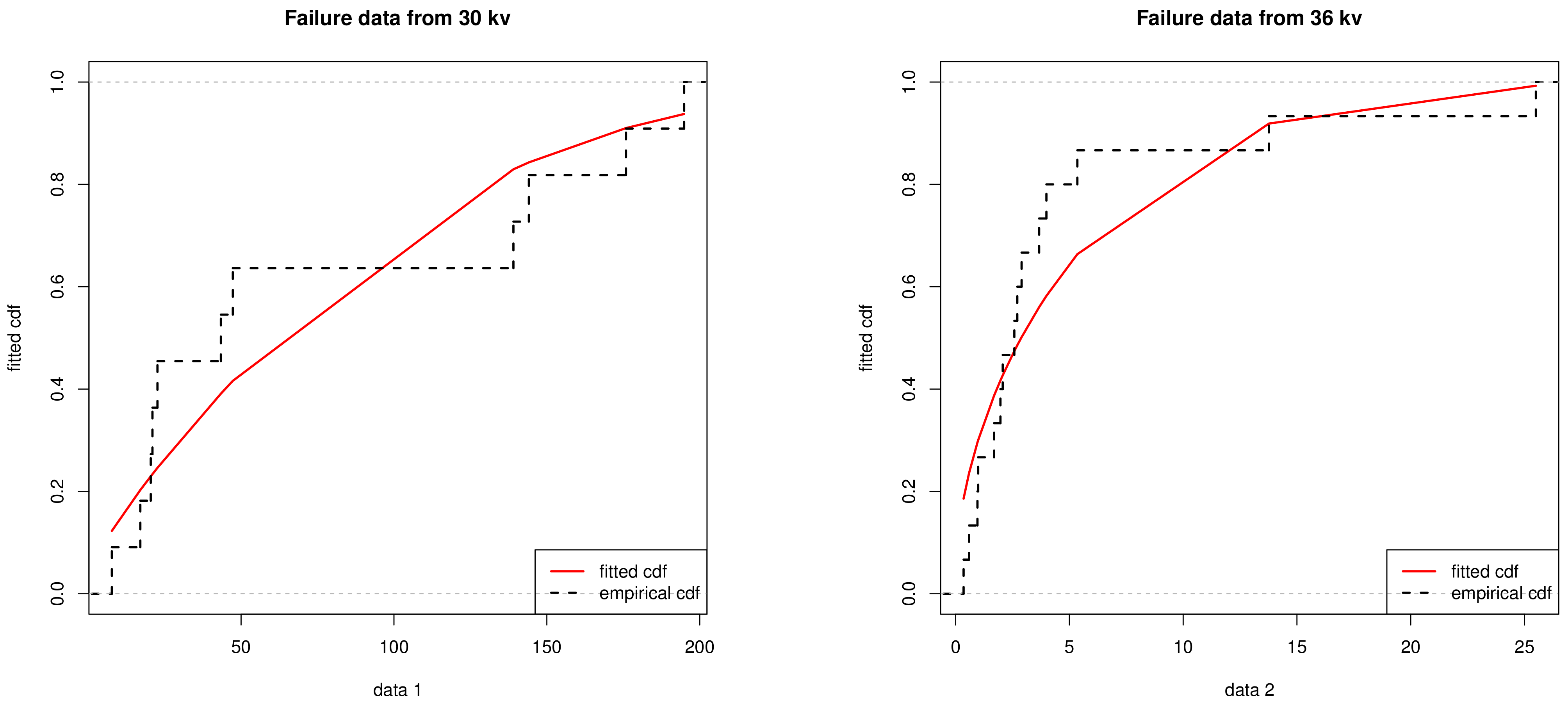
30 kV	7.74, 17.05, 20.46, 21.02, 22.66, 43.40, 47.30, 139.07, 144.12, 175.88, 194.90	0.2203	0.5858
36 kV	0.35, 0.59, 0.96, 0.99, 1.69, 1.97, 2.07, 2.58, 2.71, 2.90, 3.67, 3.99, 5.35, 13.77, 25.50	0.2179	0.4154

. To ensure the fit of the data to the Chen distribution, we calculate the Kolmogorov–Smirnov statistics and p-values, also shown in Table 9. Furthermore, the plots of the empirical cumulative distribution function and the fitted cumulative distribution function are shown in Figure 9. It is clear that the data set fits the model well.

Based on the chemical reaction mechanism leading to the failure, the inverse power model is a suitable acceleration model. Therefore, we let $\varphi \left(s_i\right)=ln\left(s_i\right)$, ($i=1,2$). The value of h is then calculated as $h=(1,1.44966)$. Under both stress levels $s_1=30$ kV and $s_2=36$ kV, the number of assigned test units $n_i$, $i=1,2$, the number of failed test units $m_i$, the progressive Type-II censoring schemes $R_i$ and the censored data are shown in

Table 10. The constant-stress progressive Type-II censored data.

Stress Level	${\mathit{h}}_{\mathit{i}}$	$\left({\mathit{n}}_{\mathit{i}},{\mathit{m}}_{\mathit{i}}\right)$	${\mathit{R}}_{\mathit{i}}$	Censored Data
30 kV	1	$\left(11,10\right)$	($0\ast 4$, 1, $0\ast 5$)	7.74, 17.05, 20.46, 21.02, 22.66, 47.30, 139.07, 144.12, 175.88, 194.90
36 kV	1.44966	$\left(15,14\right)$	($0\ast 6$, 1, $0\ast 7$)	0.35, 0.59, 0.96, 0.99, 1.69, 1.97, 2.07, 2.58, 2.90, 3.67, 3.99, 5.35, 13.77, 25.50

. The point estimates are shown in

Table 11. The maximum likelihood estimates (MLE) and the Bayes estimates using the Tierney and Kadane technique ($B{E}_{TK}$) and Lindley’s approximation ($B{E}_{LA}$).

Parameter	MLE	${\mathit{BE}}_{\mathit{TK}}$	${\mathit{BE}}_{\mathit{LA}}$
${\alpha }_0$	0.0025	0.0032	0.0026
$\lambda$	22.8063	20.4310	21.3963
$\beta$	0.2639	0.2605	0.2673

and the intervals estimates are shown in

Table 12. The 95% asymptotic confidence intervals (ACI), the 95% bootstrap percentile confidence intervals (Boot-p) and the 95% bootstrap-t confidence intervals (Boot-t).

Parameter	ACI	Boot-p	Boot-t
${\alpha }_0$	(0.0012, 0.0039) 0.0027	(0.0025, 0.0218) 0.0193	(0.0025, 0.0043) 0.0018
$\lambda$	(9.9884, 35.6241) 25.6356	(4.8530, 28.3640) 23.5111	(6.0894, 28.2857) 22.1964
$\beta$	(0.2292, 0.2986) 0.0694	(0.2162, 0.2848) 0.0686	(0.2259, 0.2812) 0.0553

. The number below each interval in Table 12 is the length of that interval. For Bayesian estimation, the results are calculated with non-informative priors in which the hyperparameters all tend to zero.

From Table 11 and Table 12, the following conclusions can be drawn:

(1)

The point estimates of ${\alpha }_0$ and $\beta$ obtained from the three different point estimation methods are similar, but the point estimates of $\lambda$ are slightly different. For $\lambda$ estimation, the MLE is maximal, followed by the BE obtained from the Lindley’s approximation and the BE obtained from the Tierney and Kadane technique;

(2)

In terms of AIL, the results obtained by the three interval estimation methods do not differ significantly. The bootstrap-t confidence intervals outperform slightly the asymptotic confidence intervals and the bootstrap percentile confidence intervals. This is consistent with the pattern that parametric bootstrap intervals outperform asymptotic intervals when the sample size is small.

(3)

For the bounds of the interval estimates of ${\alpha }_0$, the bootstrap percentile confidence intervals and the bootstrap-t confidence intervals are similar. For the interval estimates of $\lambda$, the upper and lower bounds of the asymptotic confidence intervals are significantly larger than those of the bootstrap percentile confidence intervals and the bootstrap-t confidence intervals. The bounds of the bootstrap-t confidence intervals are slightly larger than those of the bootstrap percentile confidence intervals. For the bounds on the interval estimates of $\beta$, the results obtained by the three methods are similar.

11. Conclusions

This paper considers statistical inference and optimal design of CSALT for the Chen distribution under progressive Type-II censoring. Specifically, maximum likelihood estimates are obtained utilizing the Newton–Raphson algorithm. Bayesian estimation under the squared error loss function is also considered and estimated by the Tierney and Kadane technique and Lindley’s approximation. At the same time, we establish confidence intervals for the lifetime distribution parameters and compare them. We construct the asymptotic intervals based on the observed Fisher information matrix and calculate the bootstrap percentile confidence intervals and the bootstrap-t confidence intervals to address the problem of small sample sizes. In addition, two optimal criteria are applied to determine the optimal transformed stress level that would provide more accurate estimates of the life parameters under the normal stress level. The performance of these estimation methods and the optimal criteria are compared using Monte Carlo simulation methods.

The Chen distribution possessing a bathtub-shaped hazard function is of great significance and practical importance in life experiments. Accelerated life tests and progressive censoring also play important roles. Further research into these models has great potential for estimating lifetime characteristics. This paper can also be extended by considering other distributions or other censoring schemes.

References

- McCool, J.I. Confidence limits for Weibull regression with censored data. IEEE Trans. Reliab. 1980, 29, 145–150. [Google Scholar] [CrossRef]
- Nelson, W.B. Accelerated Testing: Statistical Models, Test Plans, and Data Analysis; Wiley: New York, NY, USA, 1990. [Google Scholar]
- Miller, R.; Nelson, W. Optimum simple step-stress plans for accelerated life testing. IEEE Trans. Reliab. 1983, 32, 59–65. [Google Scholar] [CrossRef]
- Ismail, A.A. Reliability analysis under constant-stress partially accelerated life tests using hybrid censored data from Weibull distribution. Hacet. J. Math. Stat. 2016, 45, 181–193. [Google Scholar] [CrossRef]
- El-Din, M.M.M.; Abu-Youssef, S.E.; Ali, N.S.A.; El-Raheem, A.M.A. Optimal plans of constant-stress accelerated life tests for the Lindley distribution. J. Test. Eval. 2017, 45, 1463–1475. [Google Scholar]
- El-Din, M.M.M.; Abu-Youssef, S.E.; Ali, N.S.A.; El-Raheem, A.M.A. Parametric inference on step-stress accelerated life testing for the extension of exponential distribution under progressive type-II censoring. Commun. Stat. Appl. Methods 2016, 23, 269–285. [Google Scholar] [CrossRef] [Green Version]
- Chandra, N.; Khan, M.A. Analysis and optimum plan for 3-step step-stress accelerated life tests with Lomax model under progressive type-I censoring. Commun. Math. Stat. 2018, 6, 73–90. [Google Scholar]
- Abdel-Hamid, A.H.; Abushal, T.A. Inference on progressive-stress model for the exponentiated exponential distribution under type-II progressive hybrid censoring. J. Stat. Comput. Simul. 2015, 85, 1165–1186. [Google Scholar] [CrossRef]
- Balakrishnan, N.; Aggarwala, R. Progressive Censoring: Theory, Methods, and Applications; Birkhäuser: Boston, MA, USA, 2000. [Google Scholar]
- Balakrishnan, N. Progressive censoring methodology: An appraisal. Test 2007, 16, 211–259. [Google Scholar] [CrossRef]
- Jaheen, Z.F.; Moustafa, H.M.; Abd El-Monem, G.H. Bayes inference in constant partially accelerated life tests for the generalized exponential distribution with progressive censoring. Commun. Stat.-Theory Methods 2014, 43, 2973–2988. [Google Scholar] [CrossRef]
- Basak, I.; Balakrishnan, N. Prediction of censored exponential lifetimes in a simple step-stress model under progressive Type II censoring. Comput. Stat. 2017, 32, 1665–1687. [Google Scholar] [CrossRef]
- Abd El-Raheem, A.M. Inference and optimal design of multiple constant-stress testing for generalized half-normal distribution under type-II progressive censoring. J. Stat. Comput. Simul. 2019, 89, 3075–3104. [Google Scholar] [CrossRef]
- Algarni, A.; Almarashi, A.M.; Okasha, H.; Ng, H.K.T. E-bayesian estimation of Chen distribution based on type-I censoring scheme. Entropy 2020, 22, 636. [Google Scholar] [CrossRef] [PubMed]
- Chen, Z. A new two-parameter lifetime distribution with bathtub shape or increasing failure rate function. Stat. Probab. Lett. 2000, 49, 155–161. [Google Scholar] [CrossRef]
- Hjorth, U. A reliability distribution with increasing, decreasing, constant and bathtub-shaped failure rates. Technometrics 1980, 22, 99–107. [Google Scholar] [CrossRef]
- Olkin, I. Life distributions: A brief discussion. Commun. Stat.-Simul. Comput. 2016, 45, 1489–1498. [Google Scholar] [CrossRef]
- Sarhan, A.M.; Hamilton, D.C.; Smith, B. Parameter estimation for a two-parameter bathtub-shaped lifetime distribution. Appl. Math. Model. 2012, 36, 5380–5392. [Google Scholar] [CrossRef]
- Rastogi, M.K.; Tripathi, Y.M. Estimation using hybrid censored data from a two-parameter distribution with bathtub shape. Comput. Stat. Data Anal. 2013, 67, 268–281. [Google Scholar] [CrossRef]
- Ahmed, E.A. Bayesian estimation based on progressive Type-II censoring from two-parameter bathtub-shaped lifetime model: An Markov chain Monte Carlo approach. J. Appl. Stat. 2014, 41, 752–768. [Google Scholar] [CrossRef]
- Ahmed, E.A.; Alhussain, Z.A.; Salah, M.M.; Ahmed, H.H.; Eliwa, M.S. Inference of progressively type-II censored competing risks data from Chen distribution with an application. J. Appl. Stat. 2020, 47, 2492–2524. [Google Scholar] [CrossRef]
- MacDonald, I.L. Does Newton–Raphson really fail? Stat. Methods Med. Res. 2014, 23, 308–311. [Google Scholar] [CrossRef]
- Tierney, L.; Kadane, J.B. Accurate approximations for posterior moments and marginal densities. J. Am. Stat. Assoc. 1986, 81, 82–86. [Google Scholar] [CrossRef]
- Lindley, D.V. Approximate Bayesian methods. Trab. Estadística Y Investig. Oper. 1980, 31, 223–245. [Google Scholar] [CrossRef]
- Jung, M.; Chung, Y. Bayesian inference of three-parameter bathtub-shaped lifetime distribution. Commun. Stat.-Theory Methods 2018, 47, 4229–4241. [Google Scholar] [CrossRef]
- Balakrishnan, N.; Sandhu, R.A. A simple simulational algorithm for generating progressive type-II censored samples. Am. Stat. 1995, 49, 229–230. [Google Scholar]