Article

A Comprehensive Comparison of the Performance of Metaheuristic Algorithms in Neural Network Training for Nonlinear System Identification

Department of Computer Engineering, Engineering Architecture Faculty, Nevsehir Haci Bektas Veli University, Nevsehir 50300, Turkey
Mathematics 2022, 10(9), 1611; https://doi.org/10.3390/math10091611
Submission received: 6 February 2022 / Revised: 21 April 2022 / Accepted: 26 April 2022 / Published: 9 May 2022
(This article belongs to the Special Issue Neural Networks and Learning Systems II)

Abstract

:
Many problems in daily life exhibit nonlinear behavior. Therefore, it is important to solve nonlinear problems. These problems are complex and difficult due to their nonlinear nature. It is seen in the literature that different artificial intelligence techniques are used to solve these problems. One of the most important of these techniques is artificial neural networks. Obtaining successful results with an artificial neural network depends on its training process. In other words, it should be trained with a good training algorithm. Especially, metaheuristic algorithms are frequently used in artificial neural network training due to their advantages. In this study, for the first time, the performance of sixteen metaheuristic algorithms in artificial neural network training for the identification of nonlinear systems is analyzed. It is aimed to determine the most effective metaheuristic neural network training algorithms. The metaheuristic algorithms are examined in terms of solution quality and convergence speed. In the applications, six nonlinear systems are used. The mean-squared error (MSE) is utilized as the error metric. The best mean training error values obtained for six nonlinear systems were 3.5 × 10 4 , 4.7 × 10 4 , 5.6 × 10 5 , 4.8 × 10 4 , 5.2 × 10 4 , and 2.4 × 10 3 , respectively. In addition, the best mean test error values found for all systems were successful. When the results were examined, it was observed that biogeography-based optimization, moth–flame optimization, the artificial bee colony algorithm, teaching–learning-based optimization, and the multi-verse optimizer were generally more effective than other metaheuristic algorithms in the identification of nonlinear systems.

1. Introduction

In a fundamental sense, artificial intelligence can be expressed as the modeling of intelligent behavior in nature. Artificial intelligence techniques have emerged as a result of different artificial intelligence approaches. Due to the problem-solving ability of artificial intelligence techniques, artificial intelligence is used extensively in many areas [1,2,3,4].
ANNs, fuzzy logic, neuro-fuzzy, metaheuristic optimization algorithms, and deep learning are some of the artificial intelligence techniques. The fact that metaheuristic algorithms can be used together with other artificial intelligence techniques makes them powerful. ANN training, neuro-fuzzy training, or optimization of problems are examples of this situation. The computer science, bioinformatics, operation research, imaging science, food industry, meteorology, medicine, energy, education, engineering, economy, and automotive fields are some where metaheuristic algorithms are used [5,6]. When the literature is examined, it is seen that more than 200 metaheuristic algorithms have been proposed. ABC [7], BAT [8], CS [9], FPA [10], PSO [11], TLBO [12], JAYA [13], SCA [14], BBO [15], WOA [16], BSA [17], HS [18], and SSA [19] are some of the popular metaheuristic algorithms.
Many problems that we encounter in daily life exhibit nonlinear behavior. Therefore, it is important to identify these problems. When the literature is examined, it is seen that identification approaches based on network and neuro-fuzzy methods have been used. Nonlinear systems are grouped into stationary and non-stationary dynamics. Stationary stands for fixed (not depending on time) transfer functions. Non-stationary stands for the case when the transfer functions change with time [20]. Intensive studies have been carried out on nonlinear system identification. Cherkassky et al. [21] compared the performance of different methods such as ANN, KNN, GMBL, MARS, PP, and CTM on nonlinear system identification. Du ve Zhang [22] proposed an approach based on the Takagi–Sugeno (T–S) fuzzy model for the Box–Jenkins nonlinear system and nonlinear plant modeling problem. Tavoosi et al. [23] proposed a new neuro-fuzzy model called ANFIS2 for nonlinear dynamic system identification. Shoorehdeli et al. [24] introduced a hybrid neuro-fuzzy training algorithm based on PSO for the identification of nonlinear systems. Karaboga and Kaya conducted ANFIS training using the ABC algorithm for nonlinear system identification [25,26,27]. Kaya and Baştemur Kaya [28] developed a metaheuristic neural network training algorithm based on the ABC algorithm for the identification of nonlinear static systems. Subudhi and Jena [29] used an approach consisting of DE and the ANN for nonlinear system identification. Apart from these studies, there are many neuro-fuzzy- and ANN-based studies [30,31,32,33,34,35].
As seen in some of the studies above, nonlinear test functions are used to analyze the performance of many training algorithms. Nonlinear systems are inherently difficult and complex problems. Being effective in identifying nonlinear systems is one of the important indicators that training algorithms are successful. Therefore, the main subject of this study is the identification of nonlinear systems.
One of the most important techniques used in areas such as modeling, prediction, and identification is ANNs. Time series analysis, energy, air pollution prediction, the solution of engineering problems, and cancer diagnosis are some of the fields where it is utilized [36,37,38,39,40,41]. A successful training process is required to achieve effective results with the ANN. Especially, metaheuristic algorithms are used intensively in ANN training because of the good convergence speed and the absence of the local minima problem. Detailed information on the use of metaheuristic algorithms in ANN training is presented in Section 2. Different metaheuristic algorithms are preferred in solving real-world problems by utilizing the ANN. When metaheuristic algorithms are considered as neural network training algorithms, it is a fact that performance can vary depending on the type of problem. In order to determine the best training algorithm for solving the related problem, it is necessary to compare the performance of different metaheuristic algorithms. The plurality of the metaheuristic algorithm used in the comparison makes the analyzes meaningful. However, when the literature is examined, it is seen that there is a deficiency in this regard. In order to give an idea to the researchers, for the first time, ANN training is carried out with 16 metaheuristic algorithms within the scope of this study. In particular, many real-world problems exhibit nonlinear behavior. Every nonlinear system has a characteristic and may correspond to a problem in the real world. Nonlinear dynamical system identification has a long history starting from Fréchet’s theorem, where it was demonstrated that a sum of a finite number of terms of Volterra series can approximate continuous real-valued mappings. Studies on nonlinear systems have been going on for a long time [42]. Especially, nonlinear systems are inherently difficult problems. Therefore, the modeling and identification of these systems is important. The successful identification of these systems shows the success of the training algorithm. Nonlinear test systems have been used especially for the analysis of the performance of neuro-fuzzy and neural network training algorithms. In this context, the identification of nonlinear systems is chosen for the analysis of the performance of the related metaheuristic algorithms. The contributions and innovations of this study are as follows:
  • In this study, the success cases of metaheuristic algorithms are revealed. As it is known, the identification of nonlinear systems is one of the difficult problems. Which metaheuristic algorithm is more effective in solving this problem? There is no clear answer to this in the literature. Therefore, the performances of sixteen metaheuristic algorithms are compared in this study. Although this comparison is valid only for nonlinear systems, it will be a reference for different types of problems. It is thought that this study will guide the future studies of many researchers in different fields. It is an important innovation that it is one of the first studies to compare the aforementioned sixteen metaheuristic algorithms. At the same time, the results make a significant contribution to the literature.
  • The success of ANNs is directly related to the training process. In particular, metaheuristic algorithms have been used in ANN training. Some metaheuristic algorithms are heavily used, while others are more limited. However, there is no clear information about what the most effective metaheuristic-based ANN training algorithms are. This study is one of the first studies to identify the most effective metaheuristic-based ANN training algorithms. Therefore, it is innovative. The use of a training algorithm without relying on any analysis in solving a problem may be insufficient for success. This study gives an idea to the literature about which metaheuristic algorithms can be used in ANN training.
  • The importance of nonlinear systems has been emphasized above. This study is one of the most comprehensive studies in terms of the identification of nonlinear systems. It is innovative in terms of the technique used. This study was carried out on nonlinear test systems. Many systems in the real world exhibit nonlinear behavior. Therefore, this study will be a guide for the solution of many problems and will make important contributions to the literature.
This study continues as follows: Related works are presented in Section 2. Section 3 introduces the general structure of the ANN. The simulation results are presented in Section 4. The discussion is given in Section 5. The last section belongs to the conclusions.

2. Related Works

Metaheuristic algorithms are used successfully in solving difficult problems. The training of ANNs is also one of their usage areas. Recently, the increase in the number of metaheuristic algorithms has allowed the use of different metaheuristic algorithms in ANN training. Some of these algorithms are reviewed in this section:
Ozturk and Karaboga [43] proposed a hybrid approach based on the ABC algorithm and the Levenberg–Marquardt (LM) algorithm for training an ANN. Abusnaina et al. [44] proposed an approach based on the ANN and SSA to perform pattern classification. Ghanem and Jantan [45] presented a new approach based on the enhanced bat algorithm (EBat) and ANN for intrusion detection. Jaddi et al. [46] introduced a modified bat algorithm to determine the weights and structure of ANNs. The proposed algorithm was performed on classification and prediction problems. Valian et al. [47] used an improved CS to train an FFNN. Kueh and Kuok [48] trained an FFNN and recurrent neural network (RNN) by using CS to forecast long-term precipitation. Baştemur Kaya and Kaya [49] proposed an approach based on an ANN and FPA to predict the number of Turkey’s COVID-19 cases. Gupta et al. [50] suggested the usage of FPA and the generalized regression neural network (GRNN) for the prediction of COVID-19 trends. Das et al. [51] realized the training of the ANN by using PSO for nonlinear channel equalization. Ghashami et al. [52] used a hybrid approach based on an ANN and PSO for the prediction of a stock market index. Kankal and Uzlu [53] studied an ANN based on TLBO for modeling electric energy demand in Turkey. Chen et al. [54] proposed a variant of TLBO for optimizing the parameters of ANN. Wang et al. [55] trained the FFNN by using JAYA. The performance of JAYA was compared with BP, MBP, GA, SA, and PSO. Uzlu [56] suggested a hybrid algorithm based on an ANN and JAYA to estimate Turkey’s future energy usage. Hamdan et al. [57] presented an application of SCA belonging to the training of an ANN for solving a load forecasting problem. Pashiri et al. [58] used the ANN and SCA approaches for spam detection through feature selection. Pham et al. [59] utilized a new artificial intelligence technique based on a multi-layer perceptron ANN and BBO for predicting the coefficient of the consolidation of soil. Mousavirad et al. [60] proposed a hybrid neural network training algorithm based on PSO, BBO, and a global search strategy. Aljarah et al. [61] evaluated the performance of WOA in terms of solution quality and convergence speed in training the FFNN. Alameer et al. [62] used the multi-layer perceptron ANN and WOA techniques for forecasting gold price fluctuations. Aljarah et al. [63] presented an approach based on BSA and an ANN for data classification and regression applications. Xiang et al. [64] optimized a model based on an improved empirical wavelet transform (IEWT) and least-squares support vector machine (LSSVM) by using BSA for forecasting short-term wind speed. Kulluk et al. [65] implemented HS for supervised training of an ANN and used FFNNs for classification problems. In a different study, a neural network training approach based on the self-adaptive global best HS was presented [66]. Muthukumar and Balamurugan [67] proposed a hybrid renewable energy system based on an ANN and BA. Bairathi and Gopalani [68] realized the training of an ANN by using SSA. Apart from these, there are ANN studies based on metaheuristic algorithms [69,70,71].

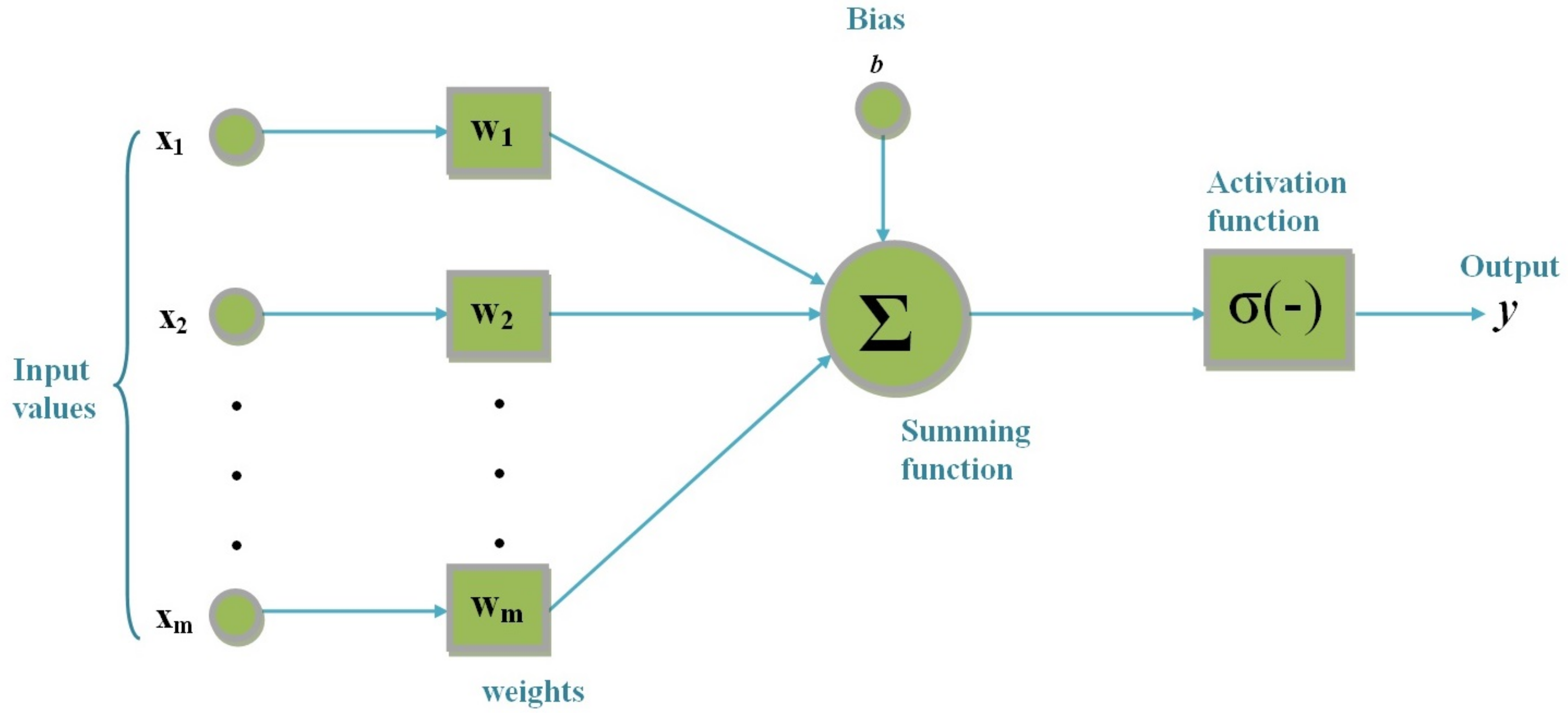
3. Artificial Neural Networks

The cornerstone of an ANN is artificial neurons. ANNs are formed by the combination of many artificial neurons. An FFNN basically consists of three layers: input, hidden, and output. There is a process in the neurons in the hidden and output layers. A neuron generates an output using the input data, as shown in Figure 1. The output of one neuron can be the input for other neurons. A neuron consists of inputs, weights, a threshold, and an output. It uses the activation and transfer functions to obtain the output value. (1) is utilized to calculate the output of the artificial neuron given in Figure 1. w is the weight value corresponding to the input. b is the bias value. f is the activation function. y corresponds to the output of the artificial neuron. Here, the summing function is used as the transfer function. In addition, there are different activation functions. One of the most popular is the sigmoid function given in (2). In this study, the sigmoid function is utilized.
y = f i = 1 m w i x i + b
σ x = 1 1 + e x
The weight and bias values in the ANN structure are important arguments of the training process. The total number of parameters to be optimized during training is directly related to these. In addition, the number of parameters to be optimized also depends on the number of inputs and the total number of neurons.
It is possible to evaluate the stage of creating the appropriate ANN structure for the solution of a problem in two steps. These are the training process and the test process. The existing sample dataset is divided into two parts. A certain part is used for the training process. The remaining part is utilized for the testing process. For a successful training process, a successful training algorithm is required. The ANN is trained using the training dataset. The maximum number of generations or an error value can be used as the stopping criterion. In simple terms, the difference between the real output and the predicted output gives the error. A low error value indicates that the training process is successful. It also means that a suitable ANN structure is obtained for solving the related problem. At the end of the training process, the ANN recognizes the training dataset. In the test process, the test is realized on the dataset that the ANN has not seen before. Therefore, the test error value is also important as the training error value.

4. Simulation Results

In this section, the results of neural network training based on metaheuristic algorithms are presented for the identification of nonlinear systems. As given in Table 1, six nonlinear systems were used. The nonlinear systems include two groups. These are stationary dynamic systems and non-stationary dynamic systems. The first four systems ( S 1 , S 2 , S 3 , and S 4 ) are stationary dynamic systems. The last two systems are non-stationary dynamic systems ( D 1 and D 2 ). S 1 has one input. S 2 and S 3 have two inputs. Other systems have three inputs. All systems consist of one output. In applications, an FFNN is used. Three different FFNN models were created for each systems. There were 5, 10 and 15 neurons utilized in the hidden layer of the FFNN. Sigmoid was used as the activation function for all neurons. The summing function was chosen as the transfer function. In addition, the bias value was utilized for each neuron. The number of data used in the training and testing process is given in Table 1. In general, 80% of the data were reserved for training. The remaining were for the testing process. Before starting the network training, the dataset was scaled in the range of [0, 1]. The colony size and maximum number of generations for all metaheuristic algorithms were 20 and 2500, respectively. Each application was run 30 times, and the mean error value was calculated. The mean-squared error (MSE) was used as the error type.
When the literature is examined, it is possible to see many nonlinear test functions. It is seen that nonlinear systems between four and ten are generally used in studies in the literature. It is not enough to describe the performance of the proposed approaches using only one system. In this context, this study included six nonlinear systems. The selected systems were taken from the literature. The input and output relationship of the system is also one of the important factors. The difference in the number of inputs also affects the network structures to be used. In fact, this completely changes the problem structure. Analyzing the proposed approaches on different systems is also a factor that increases reliability. For this reason, the analyzes were carried out on stationary dynamic systems consisting of one, two, and three inputs. The different behaviors of the stationary dynamic systems are an important reason for the preference. In fact, the equations of stationary dynamic systems give an idea about their characteristic structures. Non-stationary dynamic systems are characteristically different from stationary dynamic systems. They use past outputs/information. D 1 and D 2 are two non-stationary dynamic test functions accepted in the literature. It is possible to encounter these systems in many studies. Although both systems consist of three inputs, their characteristics are different from each other. The equation structures of systems significantly affect their characteristics. Considering this point, the systems were determined. Therefore, stationary dynamic systems based on exponential, trigonometric, and polynomial were included. On the other hand, the inputs and equation structure change the characteristic of the problem in non-stationary dynamic systems. Although both non-stationary dynamic systems consist of three inputs, their characteristics are different. This is also one of the aims of this study, namely whether the proposed approaches can produce successful solutions for different systems. Nonlinear systems are classified according to the number of inputs and outputs. All nonlinear systems used in this study contain an output. The S 1 system consists of one input. Therefore, S 1 is a SISO system. Other nonlinear systems have more than one input. Therefore, they are MISO systems. In light of this information, the identification of SISO and MISO systems was carried out within the scope of this study.
Modeling based on ANNs of nonlinear systems includes training and testing processes. In order to evaluate the performance of the obtained model, training and test results should be considered together. In the training phase, the training of the ANN is carried out on known data. In other words, the values of the weights and some parameters are determined by the training algorithm. The training process continues until the stopping criterion is met. In each generation, it is aimed to reach more optimum parameter values. As the parameter values approach the optimum, the error value will decrease. In Figure 2, a block diagram showing the modeling of a stationary dynamic system with an approach based on the ANN and metaheuristic algorithms is given. Here, s input sets are given to the system and a real output is obtained by the nonlinear system. In parallel, an estimated output value was found as a result of ANN training with metaheuristic algorithms. Until the stopping criterion, we aimed to minimize the difference between the real output and the estimated output. The same is true for non-stationary dynamic systems. Similar to stationary dynamic systems, the block diagram of modeling for non-stationary dynamic systems is given in Figure 3. In the training process, the error value or the maximum number of generations can be used as the stopping criterion. In this study, the maximum number of generations was utilized as the stopping criterion. The training process takes place on the known data set. In the testing process, data sets that are not utilized in the training of the network are used. If a successful training process has been realized, the error values belonging to the testing process should also be low.
FFNN training was performed by using sixteen metaheuristic algorithms: ABC, BAT, CS, FPA, PSO, JAYA, TLBO, SCA, BBO, WOA, BSA, HS, BA, MVO, MFO, and SSA. The results obtained for S 1 are presented in Table 2. When ABC, FPA, BBO, MVO, MFO, and SSA were used, increasing the number of neurons mostly improved the solution quality of the training and testing process. In these algorithms, the best error value was found with the 1-15-1 network structure. The training error values of CS and BA improved as the number of neurons increased. The same effect was not observed in the test error value. In these algorithms, the best result was obtained with the 1-15-1 network structure for training, while the 1-10-1 network structure was more effective for testing. As seen in the training and test results of BAT, TLBO, and BSA, the 1-10-1 network structure was more effective than other network structures. Increasing the number of neurons in PSO, SCA, and HS mostly reduced the quality of the solution. When the training and test error values were examined, the most effective results were obtained using 1-5-1 in these algorithms. The best training and test error values in JAYA and WOA were found with 1-10-1.
The results obtained for S 2 are presented in Table 3. In only five algorithms, BAT, BBO, MVO, MFO, and SSA, increasing the number of neurons positively affected the training and test results mostly. The best errors were found with the 2-15-1 network structure in these algorithms. In S 2 , CS exhibited similar behavior to S 1 . FPA was like CS. In PSO, JAYA, SCA, and HS, the training and test errors were also negatively affected by an increase in the number of neurons. The best errors for ABC, TLBO, and BSA were achieved using the 2-10-1 network structure. In WOA and BA, the change in network structure affected the training and test results differently.
The results obtained for S 3 are presented in Table 4. In BAT, BSA, and SSA, the best errors were found with 2-15-1. The increase in the number of neurons mostly improved the solution quality in these algorithms. The increase in the number of neurons for CS, FPA, PSO, SCA, WOA, HS, JAYA, and BA generally decreased the solution quality. The 2-10-1 network structure was more effective for MFO and BBO. In other algorithms, variable behavior was exhibited for the training and test processes.
The results obtained for S 4 are presented in Table 5. Reducing the number of neurons in BAT, PSO, JAYA, SCA, WOA, HS, and BA mostly improved the quality of the solution in both training and testing. The best error values were obtained by using the 3-15-1 network structure in BSA, MVO, MFO, and SSA. In these algorithms, the increase in the number of neurons positively affected the quality of the solution generally. In ABC, the best training and testing results were found with 3-10-1. In other algorithms, the change in the network structure affected the training and test results differently.
The results obtained for D 1 are presented in Table 6. The 3-15-1 network structure for ABC, BAT, BSA, MVO, MFO, and SSA was effective in both the training and test results. The 3-15-1 structure was very successful compared to 3-5-1 in these algorithms. The opposite was true for PSO, JAYA, SCA, BBO, WOA, and HS. In these algorithms, the 3-5-1 network structure was mostly more successful than the others. In TLBO, BA, and FPA, the best solutions were found in the hidden layer with ten neurons. The 3-5-1 and 3-10-1 networks were effective in CS.
The results obtained for D 2 are presented in Table 7. ABC, BAT, CS, FPA, MVO, MFO, and SSA responded positively to an increase in the number of neurons. This increased the quality of the solution for both training and testing. The best errors in PSO, SCA, WOA, and HS were obtained with the 3-5-1 network structure. The 3-10-1 network structure was effective for JAYA, TLBO, BBO, BSA, and BA.
For better analysis of the results, the best results obtained with the relevant metaheuristic algorithms are presented in Table 8, Table 9, Table 10 and Table 11. Table 8 and Table 9 refer to the training results. Table 10 and Table 11 show the test results. When the training results were examined, the eight metaheuristic algorithms for S 1 achieved the best results with the 1-15-1 network structure. The best training error value in S 1 was found as 3.5 × 10 4 by using MFO. In addition, it was observed that the 1-10-1 and 1-15-1 network structures were in competition in the test results of S 1 . As in the training error value of S 1 , the best error value in testing belonged to MFO. The performance of the metaheuristic algorithms in S 2 varied according to the network structure. Successful training error values were found with BBO, MVO, MFO, and ABC in S 2 . The best training error of S 2 belonged to BBO. In the test results, PSO, MFO, and MVO stood out. The test error value of PSO was 1.8 × 10 3 . According to the training results of S 3 , the metaheuristic algorithms seemed to be more effective mostly in 2-5-1. The best training error value was found with TLBO in S 3 . TLBO had an error value of 10 5 only. As in the training results of S 3 , 2-5-1 was also more prominent in the test results. In the test results of S 3 , PSO was quite successful compared to the other algorithms. The test error value of PSO was 2.1 × 10 4 . As in S 3 , TLBO was also very successful in the training process of S 4 . The training error value of the TLBO was 4.8 × 10 4 . At the same time, TLBO showed the same success in testing. ABC, BBO, and MFO were successful in the training process of D 1 . The best training error value was found as 5.2 × 10 4 by using BBO in D 1 . The test error value of BBO was also better than other algorithms in this system. It was 6.1 × 10 4 . There were mostly more successful results for 3-15-1 in D 2 . The effective training and test error values were obtained with MFO and BBO in D 2 . The training results of both were 2.4 × 10 3 . The test results of both were 2.5 × 10 3 .
A success ranking was created to evaluate the performance of the metaheuristic algorithms on all systems. The success ranking of the training results is given in Table 12. The best training score belonged to BBO. It was 10. After BBO, the other successful algorithms were MFO, TLBO, ABC, and MVO, respectively. The most unsuccessful algorithm in the training process was JAYA. The success ranking of the test results is given in Table 13. According to the test results, the most successful algorithm was BBO with a 16 ranking score. ABC, TLBO, MFO, and MVO followed this algorithm. The most unsuccessful algorithm was JAYA. The general success scores were created by evaluating the training and test scores together. This is presented in Table 14. The results were evaluated in three groups. Group 1 contained the most successful algorithms. These algorithms were BBO, MFO, ABC, TLBO, and MVO. The algorithms that had scores in the range of [0–70] were in this group. Group 2 was the moderately successful algorithms. The algorithms CS, SSA, PSO, FPA, and SCA were in this group. They had a score in the range of [70, 140]. Group 3 included the most unsuccessful algorithms. They were WOA, BAT, HS, BSA, BA, and JAYA.
The convergence speeds of the algorithms in Group 1 were also examined. The convergence graphs obtained for all systems are given in Figure 4, Figure 5, Figure 6, Figure 7, Figure 8 and Figure 9. It is clearly seen that the convergence speed of BBO was better in S 1 , S 2 , S 4 , and D 1 . The convergence speeds of BBO and TLBO in S 3 were close to each other. In D 2 , the convergence speeds of BBO and MFO were close to each other. TLBO had the best convergence in S 3 and S 4 , after BBO. In other systems, its position changed according to the number of generations. It was observed that ABC and MFO ranked third or forth in terms of convergence speed usually, except D 2 . MVO was in the last place in terms of convergence speed, outside D 2 .

5. Discussion

Two groups of nonlinear systems were used in the study. These were stationary dynamic systems and non-stationary dynamic systems. Both types of problems have different degrees of difficulty due to their structure. According to the best training results obtained, the error values obtained for stationary dynamic systems were more successful than non-stationary dynamic systems mostly. The best error values obtained for S 1 , S 2 , S 3 , and S 4 were 3.5 × 10 4 , 4.7 × 10 4 , 5.6 × 10 5 , and 4.8 × 10 4 , respectively. The error values of D 1 and D 2 were 5.2 × 10 4 and 2.4 × 10 3 . These error values belonged to the best results. When evaluated in terms of all metaheuristic algorithms, the success situations in nonlinear systems varied. This is a result of the general character of the algorithms. It also affects the training process. A robust behavior is expected to be exhibited in the face of all kinds of problems with metaheuristic algorithms. When evaluated in terms of six nonlinear systems, it was seen that BBO, MFO, ABC, TLBO, and MVO were effective on all systems. The network structure used was one of the important factors affecting the performance. In the applications, three different network structures were used for each system. More effective results were obtained mostly with networks that had many neurons (10 and 15). This shows that more parameters (weights) are needed for identification due to the complex structure of the problems.
Derivative-based and metaheuristic algorithms are used in ANN training. Both training approaches have some advantages and disadvantages. Derivative-based approaches have the risk of being stuck at a local minimum. This creates a significant disadvantage. The success of metaheuristic algorithms in solving difficult problems is one of the important reasons for their use in ANN training. In metaheuristic algorithms, the initial solution starts randomly. At the same time, each application is run 30 times and the mean error is found. In this study, a common comparison was not made due to the different structures of derivative-based and metaheuristic algorithms. For a fair comparison, ANN training was performed using only metaheuristic algorithms, and the performance analysis was realized. In fact, this status is one of the limitations of the study.
Besides the solution quality of metaheuristic algorithms, runtime is also an important metric. However, the time required for each application in ANN training is high. This time increases even more when each application is run 30 times. In particular, the low performance of the computer used can increase this time even more. Especially, different network structures can be tried for each system, and the effect of different control parameters on performance can be examined. These make the process even longer. Therefore, in studies where ANN and neuro-fuzzy algorithms are trained by using metaheuristic algorithms, the runtime is usually not given. Solution quality and convergence speed are used as success criteria. We evaluated our study in this direction.
The long runtime of metaheuristic algorithms in ANN training brings up the online/offline running situation. In the case of the constant change of data sets, a new training process is needed to update the network. In this case, it is more advantageous to use training algorithms with a short runtime. Every system does not require online running. If the data sets are within certain ranges, the created model can be used offline. Nonlinear systems can be evaluated in this way. The output of nonlinear systems used in the study was within a certain range. The models formed as a result of the training process can be used in offline applications. The use of metaheuristic approaches can be advantageous for the identification of nonlinear systems. Nonlinear systems are a difficult problem type by nature. At the same time, they are also a good problem type for evaluating the performance of metaheuristic algorithms. They can be used in system identification studies to evaluate the performance of the new metaheuristic approach. These studies focus on solution quality and convergence speed rather than online/offline use. In this context, a similar strategy was followed in this study.
The limitations of the study were the colony size, the maximum number of generations, the network structures used, the number of nonlinear systems utilized in identification, and the number of metaheuristic algorithms examined. The colony size was taken as 20. This value is one of the colony size values used extensively in the literature. The maximum number of generations was taken as 2500. The maximum number of generations is also one of the control parameters that affects the performance. The performances of the algorithms may vary according to this control parameter. While some metaheuristic algorithms can be effective at a low number of generations, others can be effective at a higher number of generations. Testing different maximum numbers of generations allows more precise analysis. However, this provides disadvantages in terms of time and cost. Therefore, the maximum number of generations has a limitation. The change of the network structure also affects the number of parameters to be optimized during training. A low number of parameters may be sufficient for modeling some systems. In some systems, larger network structures may be required. The performance of the model may vary depending on the number of neurons in the hidden layer. It is practically impossible to obtain a result for each different network structure. Therefore, the number of neurons in the hidden layer is one of the limitations of the study. The results belonging to one system are not sufficient to determine whether a training algorithm is successful in system identification. In system identification studies, it is seen that nonlinear systems between four and ten are generally used in the literature. In parallel with this information, six nonlinear systems were utilized in this study, and the limitation was applied. Sixteen metaheuristic algorithms were used in ANN training. This study aimed to find the most successful ones among sixteen metaheuristic algorithms. Apart from these algorithms, there may be more effective training algorithms. In addition to these, the performance of metaheuristic algorithms on nonlinear system identification was analyzed in this study. It is possible to reach different results with metaheuristic algorithms for different problems. The performance of the algorithms should be evaluated specifically for the problem at hand.
In future studies, the study can be expanded by considering these limitations. Different perspectives can be brought. In this study, only the performance of metaheuristic algorithms on nonlinear test problems was evaluated. Health, economics, engineering, education, and social sciences are some of the fields where ANN and metaheuristic algorithms are used. The approaches can be utilized for solving many problems in these areas. In addition, sixteen metaheuristic algorithms were used in this study. As is known, there are more than 200 metaheuristic algorithms in the literature. The pool of metaheuristic algorithms that was analyzed can be expanded.

6. Conclusions

Derivative-based and metaheuristic algorithms are intensely used in ANN training. Derivative-based algorithms have a risk of local minima. This situation has increased the interest in metaheuristic algorithms in ANN training. Therefore, this study focused on the performance of metaheuristic algorithms in ANN training. In this context, ANN training was carried out by using sixteen metaheuristic algorithms for the identification of nonlinear systems. The following main conclusions were reached:
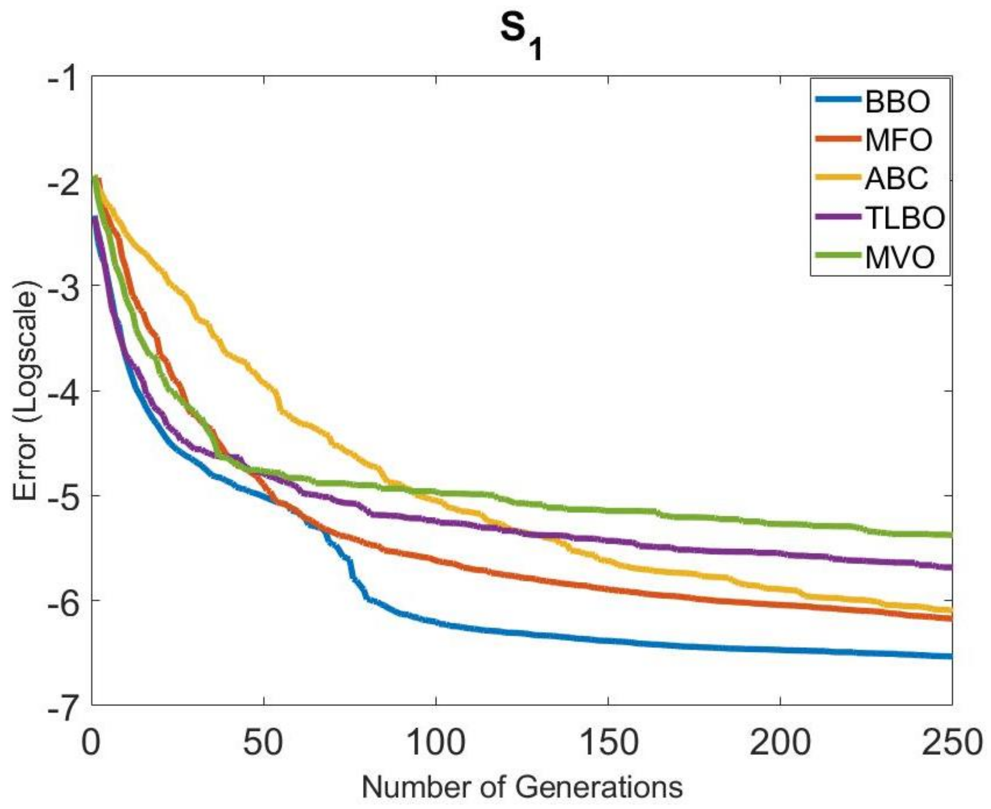
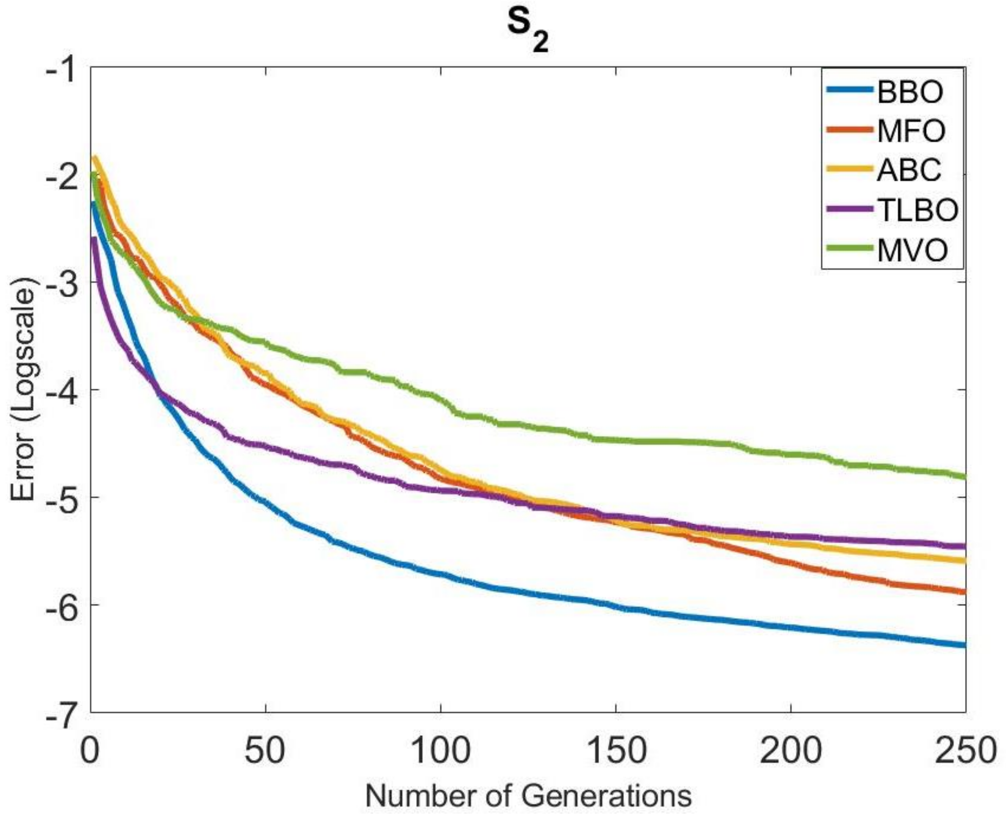
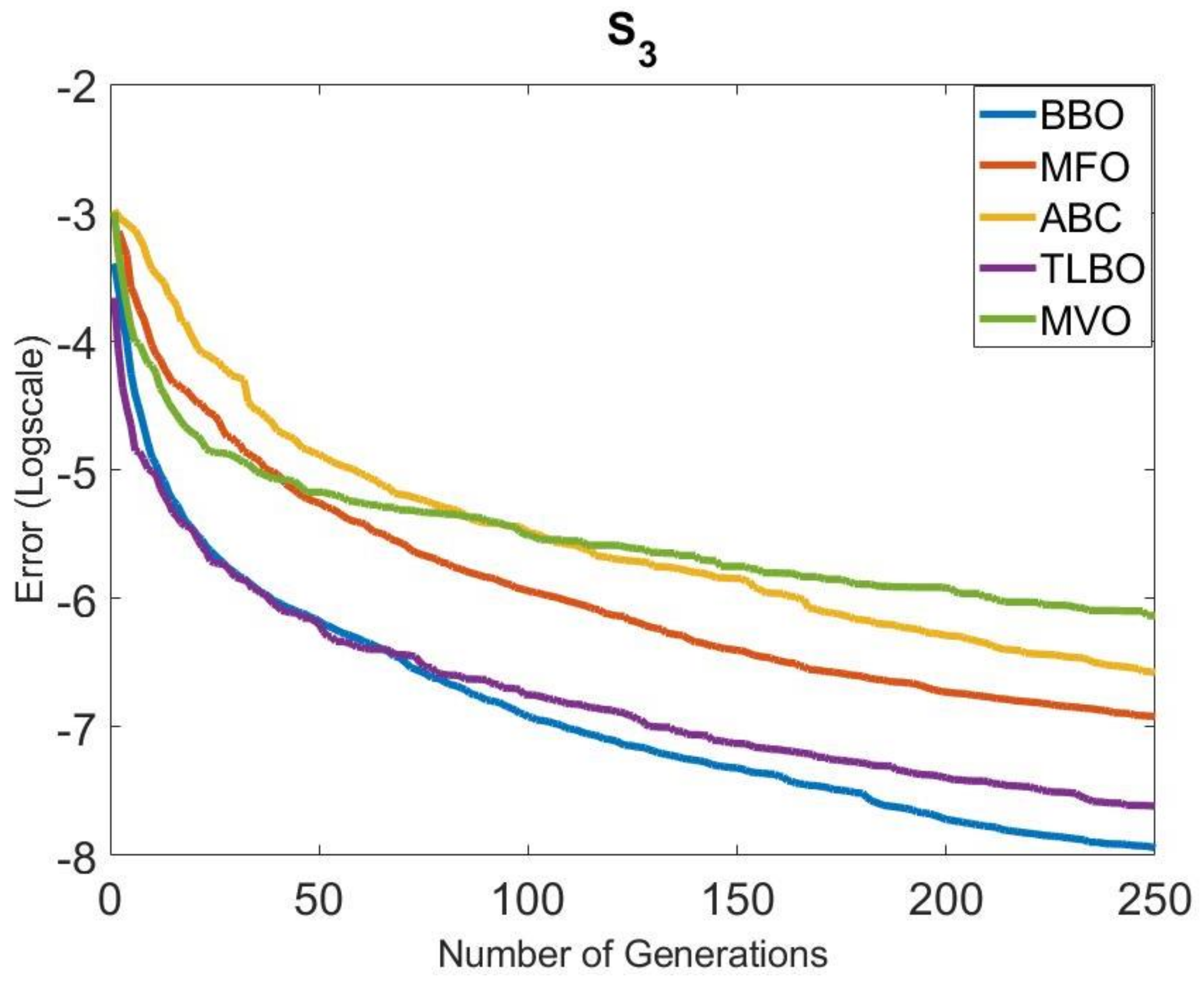
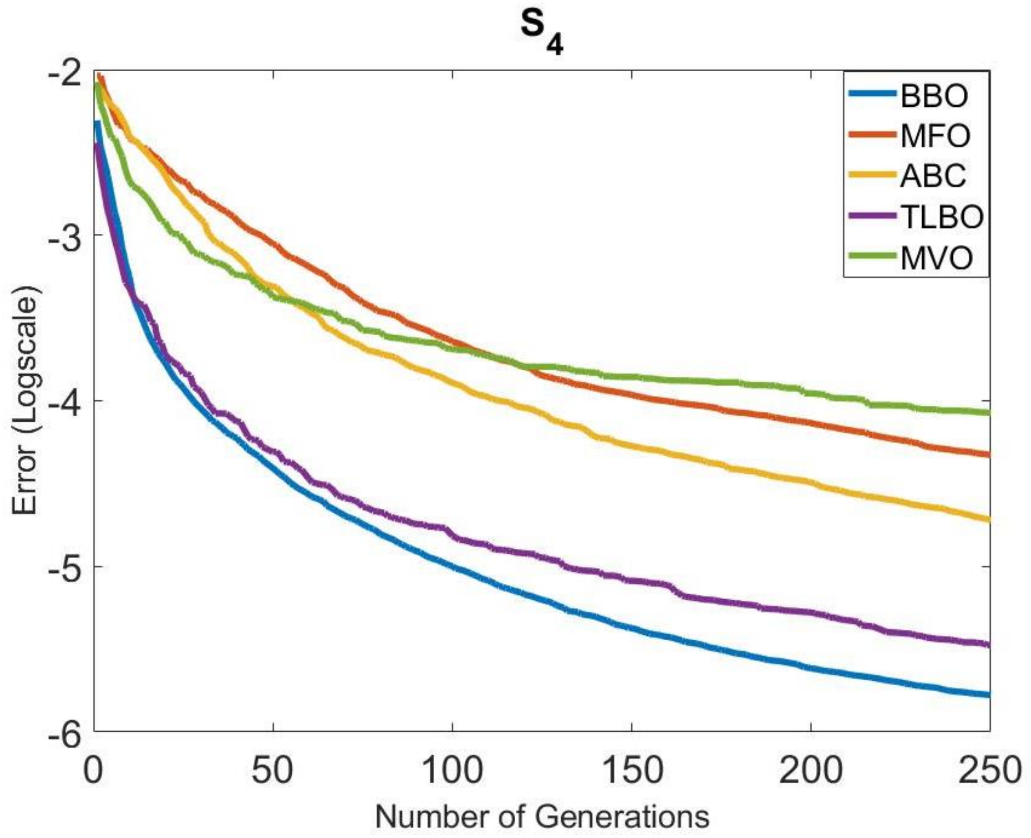
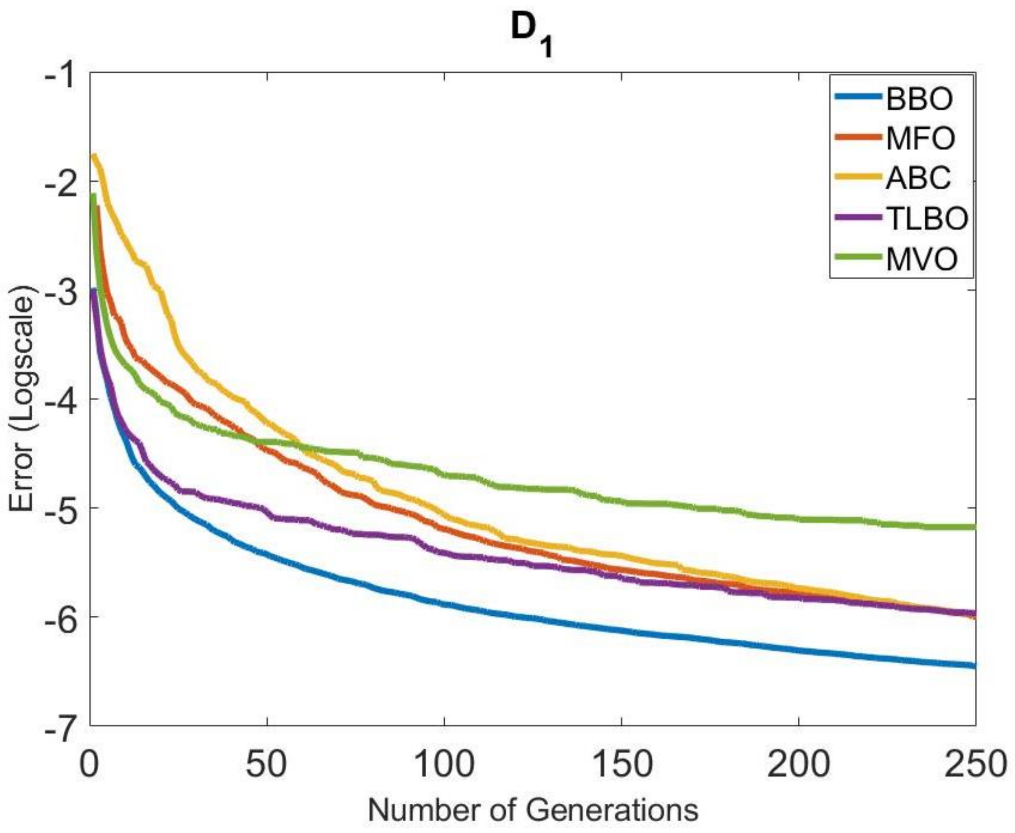
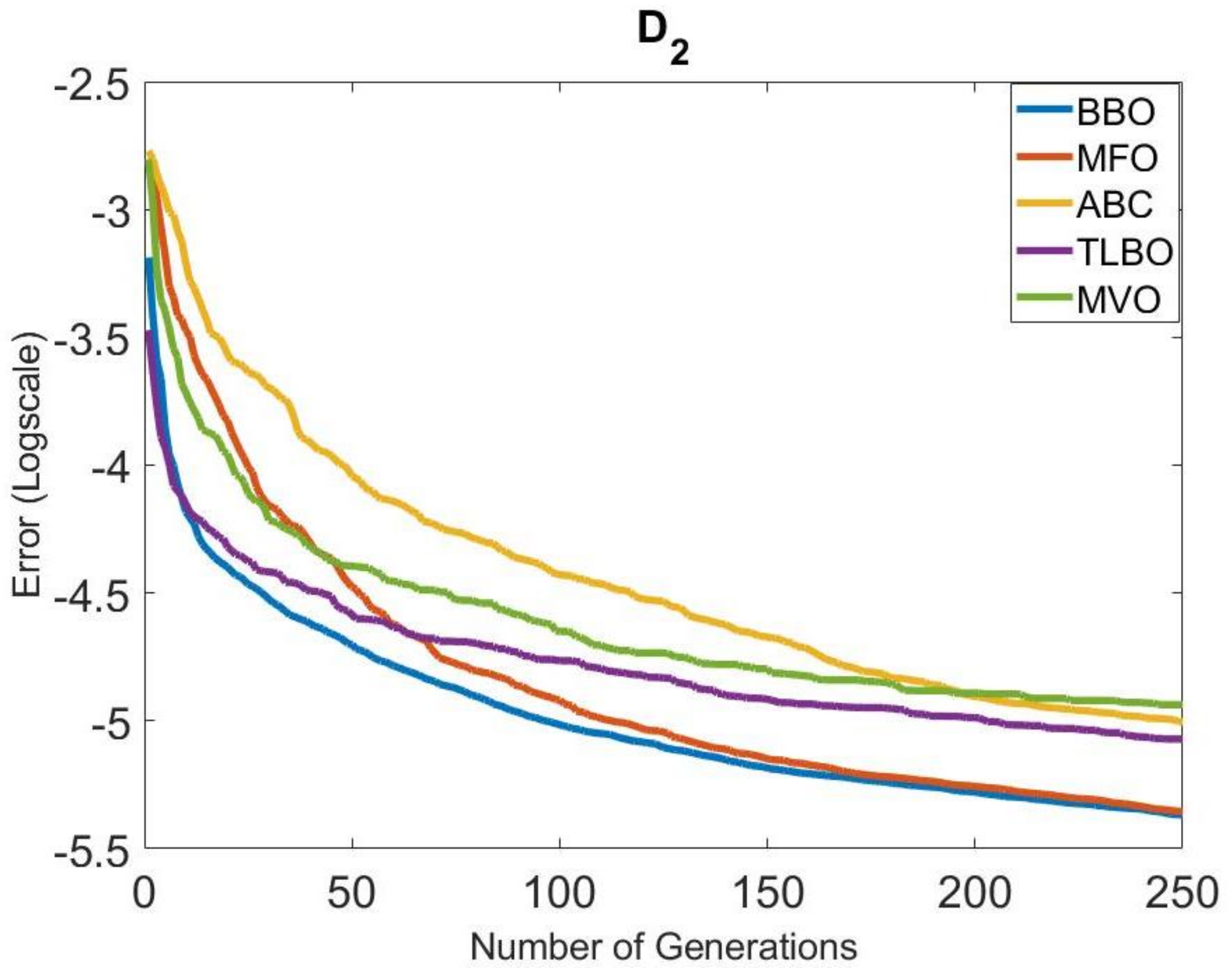
  • The performances of metaheuristic algorithms were examined in three groups. BBO, MFO, ABC, TLBO, and MVO were in Group 1. The most effective results were obtained with these algorithms. The algorithms CS, SSA, PSO, FPA, and SCA were in Group 2. Compared to Group 3, acceptable results were achieved in Group 2. The algorithms WOA, BAT, HS, BSA, BA, and JAYA were included in Group 3. It was seen that these algorithms were ineffective in solving the related problem. All rankings were valid within the stated limitations of the study.
  • The type of nonlinear systems, network structures, and training/testing processes affected the performance of the algorithms.
  • Nonlinear system identification is a difficult problem due to its structure. It was determined that most algorithms that were successful in solving numerical optimization problems cannot show the same resistance in system identification.
  • The speed of convergence is also an important criterion. The speed of convergence was very good, as was the solution quality of BBO.
In this study, ANN training was only carried out by utilizing metaheuristic algorithms for system identification. The ANN is used to solve many problems. Similarly, it is possible to carry out different studies in the future. Namely, ANN and related metaheuristic algorithms can be used for solving different problems also.

Funding

This research received no external funding.

Institutional Review Board Statement

This research did not involve humans or animals.

Informed Consent Statement

Not applicable.

Data Availability Statement

Not applicable.

Conflicts of Interest

The author declares no conflict of interest.

Abbreviations

The following abbreviations are used in this manuscript:
ABCArtificial bee colony
BATBat algorithm
CSCuckoo search
FPAFlower pollination algorithm
PSOParticle swarm optimization
TLBOTeaching–learning-based optimization
JAYAJaya algorithm
SCASine-cosine algorithm
BBOBiogeography-based optimization
WOAWhale optimization algorithm
BSABird swarm algorithm
HSHarmony search
SSASalp swarm algorithm
BABee algorithm
MFOMoth-flame optimization
MVOMulti-verse optimizer
ANNsArtificial neural networks
FFNNFeedforward neural network

References

  1. Fethi, M.D.; Pasiouras, F. Assessing bank efficiency and performance with operational research and artificial intelligence techniques: A survey. Eur. J. Oper. Res. 2010, 204, 189–198. [Google Scholar] [CrossRef]
  2. Alizadehsani, R.; Khosravi, A.; Roshanzamir, M.; Abdar, M.; Sarrafzadegan, N.; Shafie, D.; Khozeimeh, F.; Shoeibi, A.; Nahavandi, S.; Panahiazar, M. Coronary artery disease detection using artificial intelligence techniques: A survey of trends, geographical differences and diagnostic features 1991–2020. Comput. Biol. Med. 2021, 128, 104095. [Google Scholar] [CrossRef] [PubMed]
  3. Ganesh Babu, R.; Amudha, V. A Survey on Artificial Intelligence Techniques in Cognitive Radio Networks. In Emerging Technologies in Data Mining and Information Security; Abraham, A., Dutta, P., Mandal, J., Bhattacharya, A., Dutta, S., Eds.; Springer: Singapore, 2019; pp. 99–110. [Google Scholar]
  4. Bannerjee, G.; Sarkar, U.; Das, S.; Ghosh, I. Artificial Intelligence in Agriculture: A Literature Survey. Int. J. Sci. Res. Comput. Sci. Appl. Manag. Stud. 2018, 7, 1–6. [Google Scholar]
  5. Abdel-Basset, M.; Shawky, L.A. Flower pollination algorithm: A comprehensive review. Artif. Intell. Rev. 2019, 52, 2533–2557. [Google Scholar] [CrossRef]
  6. Karaboga, D.; Gorkemli, B.; Ozturk, C.; Karaboga, N. A comprehensive survey: Artificial bee colony (ABC) algorithm and applications. Artif. Intell. Rev. 2014, 42, 21–57. [Google Scholar] [CrossRef]
  7. Karaboga, D.; Basturk, B. On The performance of Artificial Bee Colony (ABC) algorithm. Appl. Soft Comput. 2008, 8, 687–697. [Google Scholar] [CrossRef]
  8. Yang, X.S. A new metaheuristic bat-inspired algorithm. In Nature Inspired Cooperative Strategies for Optimization (NICSO 2010); Springer: Berlin, Germany, 2010; pp. 65–74. [Google Scholar]
  9. Yang, X.; Deb, S. Cuckoo search via Lévy flights. In Proceedings of the IEEE World Congress on Nature & Biologically Inspired Computing (NaBIC 2009), Coimbatore, India, 9–11 December 2009; pp. 210–214. [Google Scholar]
  10. Yang, X.S. Flower pollination algorithm for global optimization. In Unconventional Computation and Natural Computation; Springer: Berlin/Heidelberg, Germany, 2012; pp. 240–249. [Google Scholar]
  11. Kennedy, J.; Eberhart, R. Particle swarm optimization. In Proceedings of the ICNN’95—International Conference on Neural Networks, Institute of Electrical and Electronics Engineers (IEEE), Perth, Australia, 27 November–1 December 1995; Volume 4, pp. 1942–1948. [Google Scholar]
  12. Rao, R.V.; Savsani, V.J.; Vakharia, D.P. Teaching–learning-based optimization: A novel method for constrained mechanical design optimization problems. Comput. Des. 2011, 43, 303–315. [Google Scholar] [CrossRef]
  13. Rao, R. Jaya: A simple and new optimization algorithm for solving constrained and unconstrained optimization problems. Int. J. Ind. Eng. 2016, 7, 19–34. [Google Scholar]
  14. Mirjalili, S. SCA: A sine cosine algorithm for solving optimization problems. Knowl. Based Syst. 2016, 96, 120–133. [Google Scholar] [CrossRef]
  15. Simon, D. Biogeography-based optimization. IEEE Trans. Evol. Comput. 2008, 12, 702–713. [Google Scholar] [CrossRef] [Green Version]
  16. Mirjalili, S.; Lewis, A. The whale optimization algorithm. Adv. Eng. Softw. 2016, 95, 51–67. [Google Scholar] [CrossRef]
  17. Meng, X.B.; Gao, X.Z.; Lu, L.H. A new bio-inspired optimisation algorithm: Bird Swarm Algorithm. J. Exp. Theory Artif. 2016, 28, 673–687. [Google Scholar] [CrossRef]
  18. Lee, K.S.; Geem, Z.W. A new meta-heuristic algorithm for continuous engineering optimization: Harmony search theory and practice. Comput. Methods Appl. Mech. Eng. 2005, 194, 3902–3933. [Google Scholar] [CrossRef]
  19. Mirjalili, S.; Gandomi, A.H.; Mirjalili, S.Z.; Saremi, S.; Faris, H.; Mirjalili, S.M. Salp Swarm Algorithm: A bio-inspired optimizer for engineering design problems. Adv. Eng. Softw. 2017, 114, 163–191. [Google Scholar] [CrossRef]
  20. Sidorov, D. Integral Dynamical Models: Singularities, Signals & Control; World Scientific Series on Nonlinear Science Series A; Chua, L.O., Ed.; World Scientific Publ. Pte: Singapore, 2015; Volume 87. [Google Scholar]
  21. Cherkassky, V.; Gehring, D.; Mulier, F. Comparison of adaptive methods for function estimation from samples. IEEE Trans. Neural Netw. 1996, 7, 969–984. [Google Scholar] [CrossRef]
  22. Du, H.; Zhang, N. Application of evolving Takagi-Sugeno fuzzy model to nonlinear system identification. Appl. Soft Comput. 2008, 8, 676–686. [Google Scholar] [CrossRef]
  23. Tavoosi, J.; Suratgar, A.A.; Menhaj, M.B. Stable ANFIS2 for Nonlinear System Identification. Neurocomputing 2016, 182, 235–246. [Google Scholar] [CrossRef]
  24. Shoorehdeli, M.A.; Teshnehlab, M.; Sedigh, A.K.; Khanesar, M.A. Identification using ANFIS with intelligent hybrid stable learning algorithm approaches and stability analysis of training methods. Appl. Soft Comput. 2009, 9, 833–850. [Google Scholar] [CrossRef]
  25. Karaboga, D.; Kaya, E. An adaptive and hybrid artificial bee colony algorithm (aABC) for ANFIS training. Appl. Soft Comput. 2016, 49, 423–436. [Google Scholar] [CrossRef]
  26. Karaboga, D.; Kaya, E. Training ANFIS by using the artificial bee colony algorithm. Turk. J. Electr. Eng. 2017, 25, 1669–1679. [Google Scholar] [CrossRef]
  27. Karaboga, D.; Kaya, E. Training ANFIS by Using an Adaptive and Hybrid Artificial Bee Colony Algorithm (aABC) for the Identification of Nonlinear Static Systems. Arab. J. Sci. Eng. 2018, 44, 3531–3547. [Google Scholar] [CrossRef]
  28. Kaya, E.; Baştemur Kaya, C. A Novel Neural Network Training Algorithm for the Identification of Nonlinear Static Systems: Artificial Bee Colony Algorithm Based on Effective Scout Bee Stage. Symmetry 2021, 13, 419. [Google Scholar] [CrossRef]
  29. Subudhi, B.; Jena, D. A differential evolution based neural network approach to nonlinear system identification. Appl. Soft Comput. 2011, 11, 861–871. [Google Scholar] [CrossRef]
  30. Giannakis, G.; Serpedin, E. A bibliography on nonlinear system identification. Signal Process. 2001, 81, 533–580. [Google Scholar] [CrossRef]
  31. Chiuso, A.; Pillonetto, G. System identification: A machine learning perspective. Annu. Rev. Control Robot. Auton. Syst. 2019, 2, 281–304. [Google Scholar] [CrossRef]
  32. Xavier, J.; Patnaik, S.; Panda, R.C. Process Modeling, Identification Methods, and Control Schemes for Nonlinear Physical Systems—A Comprehensive Review. ChemBioEng Rev. 2021, 8, 392–412. [Google Scholar] [CrossRef]
  33. Paulo Vitor de Campos Souza, P.V. Fuzzy neural networks and neuro-fuzzy networks: A review the main techniques and applications used in the literature. Appl. Soft Comput. 2020, 92, 106275. [Google Scholar] [CrossRef]
  34. Gonzalez, J.; Yu, W. Non-linear system modeling using LSTM neural networks. IFAC PapersOnLine 2018, 51, 485–489. [Google Scholar] [CrossRef]
  35. Karaboga, D.; Kaya, E. Adaptive network based fuzzy inference system (ANFIS) training approaches: A comprehensive survey. Artif. Intell. Rev. 2019, 52, 2263–2293. [Google Scholar] [CrossRef]
  36. Ambrosino, F.; Sabbarese, C.; Roca, V.; Giudicepietro, F.; Chiodini, G. Analysis of 7-years Radon time series at Campi Flegrei area (Naples, Italy) using artificial neural network method. Appl. Radiat. Isot. 2020, 163, 109239. [Google Scholar] [CrossRef]
  37. Elsheikh, A.H.; Sharshir, S.W.; Elaziz, M.A.; Kabeel, A.E.; Guilan, W.; Zhang, H. Modeling of solar energy systems using artificial neural network: A comprehensive review. Sol. Energy 2019, 180, 622–639. [Google Scholar] [CrossRef]
  38. Cabaneros, S.M.; Calautit, J.K.; Hughes, B.R. A review of artificial neural network models for ambient air pollution prediction. Environ. Model. Softw. 2019, 119, 285–304. [Google Scholar] [CrossRef]
  39. Moayedi, H.; Mosallanezhad, M.; Rashid, A.S.A.; Jusoh, W.A.W.; Muazu, M.A. A systematic review and meta-analysis of artificial neural network application in geotechnical engineering: Theory and applications. Neural Comput. Appl. 2020, 32, 495–518. [Google Scholar] [CrossRef]
  40. Bharati, S.; Podder, P.; Mondal, M. Artificial neural network based breast cancer screening: A comprehensive review. arXiv 2020, arXiv:2006.01767. [Google Scholar]
  41. Ma, S.W.; Zhang, X.; Jia, C.; Zhao, Z.; Wang, S.; Wanga, S. Image and Video Compression with Neural Networks: A Review. IEEE Trans. Circuits Syst. Video Technol. 2019, 30, 1683–1698. [Google Scholar] [CrossRef] [Green Version]
  42. Sidorov, D.N.; Sidorov, N.A. Convex majorants method in the theory of nonlinear Volterra equations. Banach J. Math. Anal. 2012, 6, 1–10. [Google Scholar] [CrossRef]
  43. Ozturk, C.; Karaboga, D. Hybrid artificial bee colony algorithm for neural network training. In Proceedings of the 2011 IEEE Congress of Evolutionary Computation (CEC), New Orleans, LA, USA, 5–8 June 2011; Volume 30, pp. 84–88. [Google Scholar]
  44. Abusnaina, A.A.; Ahmad, S.; Jarrar, R.; Mafarja, M. Training neural networks using salp swarm algorithm for pattern classification. In Proceedings of the 2nd International Conference on Future Networks and Distributed Systems, Amman, Jordan, 26–27 June 2018; p. 17. [Google Scholar]
  45. Ghanem, W.A.; Jantan, A. A new approach for intrusion detection system based on training multilayer perceptron by using enhanced Bat algorithm. Neural Comput. Appl. 2019, 32, 1–34. [Google Scholar] [CrossRef]
  46. Jaddi, N.S.; Abdullah, S.; Hamdan, A.R. Optimization of neural network model using modified bat-inspired algorithm. Appl. Soft Comput. J. 2015, 37, 71–86. [Google Scholar] [CrossRef]
  47. Valian, E.; Mohanna, S.; Tavakoli, S. Improved Cuckoo Search Algorithm for Feedforward Neural Network Training. Int. J. Artif. Intell. Appl. 2009, 2, 36–43. [Google Scholar]
  48. Kueh, S.M.; Kuok, K.K. Forecasting Long Term Precipitation Using Cuckoo Search Optimization Neural Network Models. Environ. Eng. Manag. J. 2018, 17, 1283–1291. [Google Scholar] [CrossRef]
  49. Baştemur Kaya, C.; Kaya, E. A Novel Approach Based to Neural Network and Flower Pollination Algorithm to Predict Number of COVID-19 Cases. Balkan J. Electr. Comput. Eng. 2021, 9, 327–336. [Google Scholar] [CrossRef]
  50. Gupta, K.D.; Dwivedi, R.; Sharma, D.K. Prediction of Covid-19 trends in Europe using generalized regression neural network optimized by flower pollination algorithm. J. Interdiscip. Math. 2021, 24, 33–51. [Google Scholar] [CrossRef]
  51. Das, G.; Pattnaik, P.K.; Padhy, S.K. Artificial Neural Network trained by Particle Swarm Optimization for nonlinear channel equalization. Expert Syst. Appl. 2014, 41, 3491–3496. [Google Scholar] [CrossRef]
  52. Ghashami, F.; Kamyar, K.; Riazi, S.A. Prediction of Stock Market Index Using a Hybrid Technique of Artificial Neural Networks and Particle Swarm Optimization. Appl. Econ. Financ. 2021, 8, 1–8. [Google Scholar] [CrossRef]
  53. Kankal, M.; Uzlu, E. Applications, Neural network approach with teaching–learning-based optimization for modeling and forecasting long-term electric energy demand in Turkey. Neural Comput. Appl. 2017, 28, 737–747. [Google Scholar] [CrossRef]
  54. Chen, D.; Lu, R.; Zou, F.; Li, S. Teaching-learning-based optimization with variable-population scheme and its application for ANN and global optimization. Neurocomputing 2016, 173, 1096–1111. [Google Scholar] [CrossRef]
  55. Wang, S.; Rao, R.V.; Chen, P.; Liu, A.; Wei, L. Abnormal Breast Detection in Mammogram Images by Feed-forward Neural Network Trained by Jaya Algorithm. Fundam. Inform. 2017, 151, 191–211. [Google Scholar] [CrossRef]
  56. Uzlu, E. Application of Jaya algorithm-trained artificial neural networks for prediction of energy use in the nation of Turkey. Energy Source Part B 2019, 14, 183–200. [Google Scholar] [CrossRef]
  57. Hamdan, S.; Binkhatim, S.; Jarndal, A.; Alsyouf, I. On the performance of artificial neural network with sine-cosine algorithm in forecasting electricity load demand. In Proceedings of the 2017 International Conference on Electrical and Computing Technologies and Applications (ICECTA), Ras Al Khaimah, United Arab Emirates, 21–23 November 2017. [Google Scholar]
  58. Pashiri, R.T.; Rostami, Y.; Mahrami, M. Spam detection through feature selection using artificial neural network and sine-cosine algorithm. Math. Sci. 2020, 14, 193–199. [Google Scholar] [CrossRef]
  59. Pham, B.T.; Nguyen, M.D.; Bui, K.-T.T.; Prakash, I.; Chapi, K.; Bui, D.T. A novel artificial intelligence approach based on Multi-layer Perceptron Neural Network and Biogeography-based Optimization for predicting coefficient of consolidation of soil. Catena 2018, 173, 302–311. [Google Scholar] [CrossRef]
  60. Mousavirad, S.J.; Jalali, S.M.J.; Ahmadian, S.; Khosravi, A.; Schaefer, G.; Nahavandi, S. Neural network training using a biogeography-based learning strategy. In International Conference on Neural Information Processing; Springer: Cham, Switzerland, 2020. [Google Scholar]
  61. Aljarah, I.; Faris, H.; Mirjalili, S. Optimizing connection weights in neural networks using the whale optimization algorithm. Soft Comput. 2018, 22, 1–15. [Google Scholar] [CrossRef]
  62. Alameer, Z.; Ewees, A.; Elsayed Abd Elaziz, M.; Ye, H. Forecasting gold price fluctuations using improved multilayer perceptron neural network and whale optimization algorithm. Resour. Policy 2019, 61, 250–260. [Google Scholar] [CrossRef]
  63. Aljarah, I.; Faris, H.; Mirjalili, S.; Al-Madi, N.; Sheta, A.; Mafarja, M. Evolving neural networks using bird swarm algorithm for data classification and regression applications. Clust. Comput. 2019, 22, 1317–1345. [Google Scholar] [CrossRef] [Green Version]
  64. Xiang, L.; Deng, Z.; Hu, A. Forecasting Short-Term Wind Speed Based on IEWT-LSSVM model Optimized by Bird Swarm Algorithm. IEEE Access 2019, 7, 59333–59345. [Google Scholar] [CrossRef]
  65. Kulluk, S.; Ozbakir, L.; Baykasoglu, A. Training neural networks with harmony search algorithms for classification problems. Eng. Appl. Artif. Intell. 2012, 25, 11–19. [Google Scholar] [CrossRef]
  66. Kulluk, S.; Ozbakir, L.; Baykasoglu, A. Self-adaptive global best harmony search algorithm for training neural networks. Procedia Comput. Sci. 2011, 3, 282–286. [Google Scholar] [CrossRef] [Green Version]
  67. Muthukumar, R.; Balamurugan, P. A Novel Power Optimized Hybrid Renewable Energy System Using Neural Computing and Bee Algorithm. Automatika 2019, 60, 332–339. [Google Scholar] [CrossRef] [Green Version]
  68. Bairathi, D.; Gopalani, D. Salp swarm algorithm (SSA) for training feed-forward neural networks. In Soft Computing for Problem Solving; Springer: Singapore, 2019; pp. 521–534. [Google Scholar]
  69. Han, F.; Jiang, J.; Ling, Q.H.; Su, B.Y. A survey on metaheuristic optimization for random single-hidden layer feedforward neural network. Neurocomputing 2019, 335, 261–273. [Google Scholar] [CrossRef]
  70. Ojha, V.K.; Abraham, A.; Snášel, V. Metaheuristic Design of Feedforward Neural Networks: A Review of Two Decades of Research. Eng. Appl. Artif. Intell. 2017, 60, 97–116. [Google Scholar] [CrossRef] [Green Version]
  71. Elaziz, M.A.; Dahou, A.; Abualigah, L.; Yu, L.; Alshinwan, M.; Khasawneh, A.M.; Lu, S. Advanced metaheuristic optimization techniques in applications of deep neural networks: A review. Neural Comput. Appl. 2021, 33, 14079–14099. [Google Scholar] [CrossRef]
Figure 1. General structure of an artificial neuron.
Mathematics 10 01611 g001
Figure 2. A block diagram of the identification of stationary dynamic systems with the proposed approaches.
Mathematics 10 01611 g002
Figure 3. A block diagram of the identification of non-stationary dynamic systems with the proposed approaches.
Mathematics 10 01611 g003
Figure 4. Comparison of the convergence of the metaheuristic algorithms in Group 1 for S 1 .
Mathematics 10 01611 g004
Figure 5. Comparison of the convergence of the metaheuristic algorithms in Group 1 for S 2 .
Mathematics 10 01611 g005
Figure 6. Comparison of the convergence of the metaheuristic algorithms in Group 1 for S 3 .
Mathematics 10 01611 g006
Figure 7. Comparison of the convergence of the metaheuristic algorithms in Group 1 for S 4 .
Mathematics 10 01611 g007
Figure 8. Comparison of the convergence of the metaheuristic algorithms in Group 1 for D 1 .
Mathematics 10 01611 g008
Figure 9. Comparison of the convergence of the metaheuristic algorithms in Group 1 for D 2 .
Mathematics 10 01611 g009
Table 1. Nonlinear systems used.
SystemEquationInputsOutputNumber of
Training/Test Data
S 1 y = 2 sin π x 1 x 1 y80\20
S 2 y = 10.391 x 1 0.4 x 2 0.6 + 0.36 x 1 , x 2 y80\20
S 3 y = tanh x 1 + x 2 11 x 1 , x 2 y80\20
S 4 y = 1 + x 1 0.5 + x 2 1 + x 3 1.5 x 1 , x 2 , x 3 y173\43
D 1 y k + 1 = y k y k 1 y k + 2.5 1 + y k 2 + y k 1 2 + u k y k , y k 1 , u k y k + 1 200\50
D 2 y k + 1 = y k 1 + y k 1 + u k 3 y k , y k 1 , u k y k + 1 200\50
Table 2. The results obtained by using the metaheuristic algorithms for S 1 .
AlgorithmNetwork StructureTrainTest
MeanSD.MeanSD.
ABC1-5-1 1.6 × 10 3 4.2 × 10 4 2.4 × 10 3 6.2 × 10 4
1-10-1 8.2 × 10 4 3.4 × 10 4 1.6 × 10 3 6.8 × 10 4
1-15-1 7.1 × 10 4 2.4 × 10 4 1.5 × 10 3 5.3 × 10 4
BAT1-5-1 2.6 × 10 2 3.6 × 10 2 3.0 × 10 2 3.8 × 10 2
1-10-1 2.2 × 10 2 3.9 × 10 2 2.3 × 10 2 4.0 × 10 2
1-15-1 2.5 × 10 2 4.6 × 10 2 2.7 × 10 2 5.0 × 10 2
CS1-5-1 1.3 × 10 3 2.2 × 10 4 2.2 × 10 3 5.1 × 10 4
1-10-1 8.0 × 10 4 2.4 × 10 4 1.6 × 10 3 5.5 × 10 4
1-15-1 7.3 × 10 4 1.7 × 10 4 1.8 × 10 3 5.8 × 10 4
FPA1-5-1 1.4 × 10 3 2.6 × 10 4 2.3 × 10 3 5.6 × 10 4
1-10-1 9.2 × 10 4 2.9 × 10 4 1.7 × 10 3 5.3 × 10 4
1-15-1 8.0 × 10 4 2.7 × 10 4 1.7 × 10 3 7.1 × 10 4
PSO1-5-1 1.7 × 10 3 4.6 × 10 4 1.7 × 10 3 4.6 × 10 4
1-10-1 2.1 × 10 3 6.2 × 10 4 2.1 × 10 3 6.2 × 10 4
1-15-1 2.1 × 10 3 6.0 × 10 4 2.1 × 10 3 6.0 × 10 4
JAYA1-5-1 1.5 × 10 2 8.3 × 10 3 1.6 × 10 2 9.0 × 10 3
1-10-1 1.3 × 10 2 6.5 × 10 3 1.4 × 10 2 7.4 × 10 3
1-15-1 1.4 × 10 2 8.3 × 10 3 1.4 × 10 2 9.3 × 10 3
TLBO1-5-1 1.1 × 10 3 6.7 × 10 4 2.0 × 10 3 1.1 × 10 3
1-10-1 9.7 × 10 4 6.5 × 10 4 1.6 × 10 3 7.7 × 10 4
1-15-1 9.9 × 10 4 5.1 × 10 4 1.6 × 10 3 6.5 × 10 4
SCA1-5-1 4.5 × 10 3 8.2 × 10 4 5.6 × 10 3 1.5 × 10 3
1-10-1 5.0 × 10 3 1.6 × 10 3 5.9 × 10 3 2.0 × 10 3
1-15-1 4.9 × 10 3 1.5 × 10 3 5.9 × 10 3 2.8 × 10 3
BBO1-5-1 9.2 × 10 4 3.9 × 10 4 1.9 × 10 3 6.5 × 10 4
1-10-1 6.9 × 10 4 2.5 × 10 4 1.6 × 10 3 4.9 × 10 4
1-15-1 5.3 × 10 4 2.3 × 10 4 1.5 × 10 3 5.2 × 10 4
WOA1-5-1 7.8 × 10 3 9.4 × 10 3 8.3 × 10 3 6.9 × 10 3
1-10-1 3.8 × 10 3 2.1 × 10 3 5.4 × 10 3 3.2 × 10 3
1-15-1 7.4 × 10 3 9.7 × 10 3 8.4 × 10 3 8.6 × 10 3
BSA1-5-1 3.0 × 10 2 2.6 × 10 2 3.3 × 10 2 2.9 × 10 2
1-10-1 9.2 × 10 3 1.8 × 10 2 1.0 × 10 2 1.7 × 10 2
1-15-1 2.7 × 10 2 3.5 × 10 2 2.8 × 10 2 3.5 × 10 2
HS1-5-1 1.1 × 10 2 1.2 × 10 2 1.2 × 10 2 1.2 × 10 2
1-10-1 2.4 × 10 2 1.6 × 10 2 2.7 × 10 2 2.0 × 10 2
1-15-1 2.7 × 10 2 1.2 × 10 2 3.0 × 10 2 1.3 × 10 2
BA1-5-1 9.0 × 10 3 3.5 × 10 3 1.1 × 10 2 4.8 × 10 3
1-10-1 6.4 × 10 3 2.3 × 10 3 7.2 × 10 3 2.8 × 10 3
1-15-1 6.2 × 10 3 2.3 × 10 3 7.8 × 10 3 3.6 × 10 3
MVO1-5-1 1.2 × 10 3 5.6 × 10 4 2.4 × 10 3 9.7 × 10 4
1-10-1 9.0 × 10 4 5.9 × 10 4 2.0 × 10 3 8.7 × 10 4
1-15-1 4.9 × 10 4 2.6 × 10 4 1.5 × 10 3 5.5 × 10 4
MFO1-5-1 1.8 × 10 3 1.4 × 10 3 2.6 × 10 3 1.5 × 10 3
1-10-1 8.2 × 10 4 8.4 × 10 4 1.7 × 10 3 1.1 × 10 3
1-15-1 3.5 × 10 4 2.7 × 10 4 1.4 × 10 3 6.9 × 10 4
SSA1-5-1 1.4 × 10 3 5.8 × 10 4 2.7 × 10 3 9.0 × 10 4
1-10-1 9.7 × 10 4 6.1 × 10 4 2.0 × 10 3 8.3 × 10 4
1-15-1 7.9 × 10 4 5.4 × 10 4 1.8 × 10 3 6.7 × 10 4
Table 3. The results obtained by using the metaheuristic algorithms for S 2 .
AlgorithmNetwork StructureTrainTest
MeanSD.MeanSD.
ABC2-5-1 9.1 × 10 4 2.9 × 10 4 5.1 × 10 3 2.3 × 10 3
2-10-1 5.4 × 10 4 1.7 × 10 4 4.1 × 10 3 2.5 × 10 3
2-15-1 7.1 × 10 4 3.9 × 10 4 5.7 × 10 3 4.1 × 10 3
BAT2-5-1 9.9 × 10 3 1.3 × 10 2 2.2 × 10 2 1.9 × 10 2
2-10-1 1.2 × 10 2 3.2 × 10 2 2.1 × 10 2 3.4 × 10 2
2-15-1 8.9 × 10 3 2.8 × 10 2 1.7 × 10 2 3.3 × 10 2
CS2-5-1 1.3 × 10 3 3.8 × 10 4 6.0 × 10 3 3.3 × 10 3
2-10-1 1.0 × 10 3 2.6 × 10 4 4.4 × 10 3 2.1 × 10 3
2-15-1 9.8 × 10 4 2.5 × 10 4 5.1 × 10 3 2.8 × 10 3
FPA2-5-1 1.6 × 10 3 5.7 × 10 4 6.4 × 10 3 3.1 × 10 3
2-10-1 1.2 × 10 3 3.2 × 10 4 5.8 × 10 3 2.9 × 10 3
2-15-1 1.1 × 10 3 2.8 × 10 4 6.0 × 10 3 3.1 × 10 3
PSO2-5-1 1.8 × 10 3 1.3 × 10 3 1.8 × 10 3 1.3 × 10 3
2-10-1 2.6 × 10 3 1.2 × 10 3 2.6 × 10 3 1.2 × 10 3
2-15-1 3.5 × 10 3 1.4 × 10 3 3.5 × 10 3 1.4 × 10 3
JAYA2-5-1 1.6 × 10 2 5.8 × 10 3 2.8 × 10 2 1.0 × 10 2
2-10-1 2.3 × 10 2 8.9 × 10 3 4.4 × 10 2 2.3 × 10 2
2-15-1 3.2 × 10 2 1.3 × 10 2 5.6 × 10 2 2.8 × 10 2
TLBO2-5-1 1.2 × 10 3 9.7 × 10 4 5.8 × 10 3 3.8 × 10 3
2-10-1 6.2 × 10 4 5.6 × 10 4 4.0 × 10 3 2.2 × 10 3
2-15-1 8.0 × 10 4 5.8 × 10 4 4.5 × 10 3 2.8 × 10 3
SCA2-5-1 7.5 × 10 3 1.3 × 10 3 1.7 × 10 2 6.7 × 10 3
2-10-1 9.2 × 10 3 2.4 × 10 3 2.2 × 10 2 6.2 × 10 3
2-15-1 1.1 × 10 2 3.3 × 10 3 2.2 × 10 2 7.3 × 10 3
BBO2-5-1 1.0 × 10 3 1.2 × 10 3 6.6 × 10 3 4.5 × 10 3
2-10-1 5.7 × 10 4 4.9 × 10 4 4.3 × 10 3 2.4 × 10 3
2-15-1 4.7 × 10 4 2.8 × 10 4 4.3 × 10 3 2.1 × 10 3
WOA2-5-1 9.1 × 10 3 5.3 × 10 3 2.4 × 10 2 7.6 × 10 3
2-10-1 9.9 × 10 3 5.5 × 10 3 2.2 × 10 2 7.7 × 10 3
2-15-1 9.7 × 10 3 5.9 × 10 3 2.1 × 10 2 6.4 × 10 3
BSA2-5-1 1.3 × 10 2 6.9 × 10 3 2.6 × 10 2 8.6 × 10 3
2-10-1 8.6 × 10 3 6.0 × 10 3 1.8 × 10 2 9.2 × 10 3
2-15-1 1.4 × 10 2 8.1 × 10 3 2.6 × 10 2 9.5 × 10 3
HS2-5-1 4.9 × 10 3 3.7 × 10 3 1.2 × 10 2 5.6 × 10 3
2-10-1 2.9 × 10 2 1.5 × 10 2 4.8 × 10 2 2.9 × 10 2
2-15-1 5.1 × 10 2 1.6 × 10 2 6.7 × 10 2 3.1 × 10 2
BA2-5-1 1.0 × 10 2 2.4 × 10 3 2.5 × 10 2 9.8 × 10 3
2-10-1 1.2 × 10 2 3.7 × 10 3 2.3 × 10 2 1.1 × 10 2
2-15-1 1.7 × 10 2 7.0 × 10 3 3.0 × 10 2 1.5 × 10 2
MVO2-5-1 2.5 × 10 3 2.1 × 10 3 1.0 × 10 2 6.9 × 10 3
2-10-1 9.2 × 10 4 6.7 × 10 4 5.5 × 10 3 4.5 × 10 3
2-15-1 5.5 × 10 4 4.0 × 10 4 3.8 × 10 3 2.6 × 10 3
MFO2-5-1 2.8 × 10 3 2.4 × 10 3 8.9 × 10 3 7.5 × 10 3
2-10-1 8.8 × 10 4 8.4 × 10 4 5.9 × 10 3 5.4 × 10 3
2-15-1 5.2 × 10 4 5.5 × 10 4 3.7 × 10 3 2.2 × 10 3
SSA2-5-1 4.0 × 10 3 2.0 × 10 3 1.2 × 10 2 7.3 × 10 3
2-10-1 1.9 × 10 3 1.5 × 10 3 7.9 × 10 3 5.5 × 10 3
2-15-1 1.2 × 10 3 1.0 × 10 3 6.7 × 10 3 3.9 × 10 3
Table 4. The results obtained by using the metaheuristic algorithms for S 3 .
AlgorithmNetwork StructureTrainTest
MeanSD.MeanSD.
ABC2-5-1 2.7 × 10 4 1.4 × 10 4 3.4 × 10 3 2.6 × 10 3
2-10-1 2.3 × 10 4 1.2 × 10 4 3.8 × 10 3 2.8 × 10 3
2-15-1 2.9 × 10 4 1.5 × 10 4 4.1 × 10 3 2.7 × 10 3
BAT2-5-1 1.6 × 10 3 2.1 × 10 3 9.5 × 10 3 6.8 × 10 3
2-10-1 3.2 × 10 3 8.4 × 10 3 1.5 × 10 2 2.4 × 10 2
2-15-1 1.6 × 10 3 4.7 × 10 3 9.2 × 10 3 7.5 × 10 3
CS2-5-1 1.4 × 10 4 4.2 × 10 5 3.5 × 10 3 1.3 × 10 3
2-10-1 2.1 × 10 4 7.9 × 10 5 4.0 × 10 3 1.3 × 10 3
2-15-1 3.0 × 10 4 9.0 × 10 5 5.0 × 10 3 2.0 × 10 3
FPA2-5-1 2.0 × 10 4 8.5 × 10 5 4.0 × 10 3 2.0 × 10 3
2-10-1 2.4 × 10 4 8.4 × 10 5 4.2 × 10 3 1.9 × 10 3
2-15-1 3.2 × 10 4 1.2 × 10 4 5.0 × 10 3 2.2 × 10 3
PSO2-5-1 2.1 × 10 4 1.6 × 10 4 2.1 × 10 4 1.6 × 10 4
2-10-1 4.1 × 10 4 2.8 × 10 4 4.1 × 10 4 2.8 × 10 4
2-15-1 7.1 × 10 4 3.1 × 10 4 7.1 × 10 4 3.1 × 10 4
JAYA2-5-1 6.2 × 10 3 3.1 × 10 3 2.4 × 10 2 1.6 × 10 2
2-10-1 8.2 × 10 3 3.1 × 10 3 2.8 × 10 2 1.8 × 10 2
2-15-1 1.1 × 10 2 3.6 × 10 3 2.9 × 10 2 1.9 × 10 2
TLBO2-5-1 5.6 × 10 5 4.1 × 10 5 2.9 × 10 3 9.2 × 10 4
2-10-1 7.1 × 10 5 7.9 × 10 5 2.8 × 10 3 1.1 × 10 3
2-15-1 1.3 × 10 4 1.0 × 10 4 4.1 × 10 3 1.5 × 10 3
SCA2-5-1 1.2 × 10 3 4.8 × 10 4 7.6 × 10 3 4.8 × 10 3
2-10-1 1.7 × 10 3 7.1 × 10 4 1.0 × 10 2 5.4 × 10 3
2-15-1 2.1 × 10 3 9.3 × 10 4 9.7 × 10 3 4.2 × 10 3
BBO2-5-1 1.1 × 10 4 8.9 × 10 5 4.0 × 10 3 1.6 × 10 3
2-10-1 1.0 × 10 4 7.5 × 10 5 3.5 × 10 3 1.7 × 10 3
2-15-1 2.0 × 10 4 2.1 × 10 4 4.7 × 10 3 1.8 × 10 3
WOA2-5-1 1.6 × 10 3 1.5 × 10 3 9.8 × 10 3 4.2 × 10 3
2-10-1 1.6 × 10 3 2.1 × 10 3 1.0 × 10 2 7.5 × 10 3
2-15-1 1.9 × 10 3 2.4 × 10 3 1.2 × 10 2 1.1 × 10 2
BSA2-5-1 4.2 × 10 3 6.8 × 10 3 1.9 × 10 2 1.8 × 10 2
2-10-1 2.3 × 10 3 2.0 × 10 3 1.4 × 10 2 8.5 × 10 3
2-15-1 2.2 × 10 3 1.9 × 10 3 1.4 × 10 2 8.4 × 10 3
HS2-5-1 2.2 × 10 3 1.7 × 10 3 1.0 × 10 2 7.5 × 10 3
2-10-1 9.5 × 10 3 2.9 × 10 3 2.6 × 10 2 1.3 × 10 2
2-15-1 1.4 × 10 2 4.0 × 10 3 3.0 × 10 2 1.6 × 10 2
BA2-5-1 2.7 × 10 3 1.1 × 10 3 9.8 × 10 3 5.4 × 10 3
2-10-1 3.5 × 10 3 1.3 × 10 3 1.3 × 10 2 5.3 × 10 3
2-15-1 4.6 × 10 3 1.5 × 10 3 1.4 × 10 2 9.8 × 10 3
MVO2-5-1 1.6 × 10 4 1.2 × 10 4 3.8 × 10 3 1.4 × 10 3
2-10-1 1.2 × 10 4 8.6 × 10 5 3.7 × 10 3 1.6 × 10 3
2-15-1 1.3 × 10 4 7.8 × 10 5 3.6 × 10 3 1.5 × 10 3
MFO2-5-1 5.1 × 10 4 9.8 × 10 4 4.5 × 10 3 4.7 × 10 3
2-10-1 2.0 × 10 4 2.7 × 10 4 4.5 × 10 3 4.2 × 10 3
2-15-1 3.2 × 10 4 4.0 × 10 4 6.3 × 10 3 6.7 × 10 3
SSA2-5-1 1.6 × 10 4 1.2 × 10 4 3.8 × 10 3 1.3 × 10 3
2-10-1 1.6 × 10 4 1.3 × 10 4 3.8 × 10 3 1.6 × 10 3
2-15-1 1.1 × 10 4 8.0 × 10 5 3.6 × 10 3 1.3 × 10 3
Table 5. The results obtained by using the metaheuristic algorithms for S 4 .
AlgorithmNetwork StructureTrainTest
MeanSD.MeanSD.
ABC3-5-1 1.9 × 10 3 6.0 × 10 4 2.3 × 10 3 8.1 × 10 4
3-10-1 1.5 × 10 3 4.6 × 10 4 2.1 × 10 3 7.3 × 10 4
3-15-1 2.0 × 10 3 1.0 × 10 3 3.1 × 10 3 1.4 × 10 3
BAT3-5-1 1.5 × 10 2 1.1 × 10 2 1.5 × 10 2 1.1 × 10 2
3-10-1 1.6 × 10 2 2.3 × 10 2 1.7 × 10 2 2.5 × 10 2
3-15-1 1.8 × 10 2 3.1 × 10 2 1.8 × 10 2 3.3 × 10 2
CS3-5-1 2.6 × 10 3 5.7 × 10 4 2.9 × 10 3 7.9 × 10 4
3-10-1 2.5 × 10 3 4.5 × 10 4 3.0 × 10 3 7.6 × 10 4
3-15-1 3.0 × 10 3 5.0 × 10 4 3.3 × 10 3 7.4 × 10 4
FPA3-5-1 3.1 × 10 3 9.1 × 10 4 3.5 × 10 3 1.1 × 10 3
3-10-1 3.2 × 10 3 6.7 × 10 4 3.5 × 10 3 1.0 × 10 3
3-15-1 3.3 × 10 3 1.0 × 10 3 3.4 × 10 3 1.2 × 10 3
PSO3-5-1 2.1 × 10 3 8.7 × 10 4 2.1 × 10 3 8.7 × 10 4
3-10-1 3.6 × 10 3 1.6 × 10 3 3.6 × 10 3 1.6 × 10 3
3-15-1 5.2 × 10 3 2.2 × 10 3 5.2 × 10 3 2.2 × 10 3
JAYA3-5-1 3.0 × 10 2 1.0 × 10 2 2.9 × 10 2 1.2 × 10 2
3-10-1 4.8 × 10 2 1.8 × 10 2 4.9 × 10 2 1.9 × 10 2
3-15-1 5.5 × 10 2 1.6 × 10 2 5.4 × 10 2 1.9 × 10 2
TLBO3-5-1 1.5 × 10 3 1.2 × 10 3 1.9 × 10 3 1.1 × 10 3
3-10-1 4.8 × 10 4 2.3 × 10 4 9.7 × 10 4 3.9 × 10 4
3-15-1 6.9 × 10 4 6.4 × 10 4 1.2 × 10 3 5.6 × 10 4
SCA3-5-1 7.5 × 10 3 2.4 × 10 3 7.6 × 10 3 2.5 × 10 3
3-10-1 9.2 × 10 3 2.7 × 10 3 9.1 × 10 3 3.0 × 10 3
3-15-1 9.6 × 10 3 3.9 × 10 3 9.4 × 10 3 3.6 × 10 3
BBO3-5-1 8.8 × 10 4 5.5 × 10 4 1.4 × 10 3 7.6 × 10 4
3-10-1 8.1 × 10 4 6.3 × 10 4 1.5 × 10 3 8.7 × 10 4
3-15-1 1.2 × 10 3 5.8 × 10 4 1.8 × 10 3 9.0 × 10 4
WOA3-5-1 8.2 × 10 3 4.8 × 10 3 8.2 × 10 3 5.1 × 10 3
3-10-1 9.4 × 10 3 7.0 × 10 3 9.4 × 10 3 7.1 × 10 3
3-15-1 9.5 × 10 3 6.5 × 10 3 9.3 × 10 3 7.4 × 10 3
BSA3-5-1 1.5 × 10 2 6.5 × 10 3 1.4 × 10 2 6.8 × 10 3
3-10-1 1.5 × 10 2 8.0 × 10 3 1.5 × 10 2 8.8 × 10 3
3-15-1 1.4 × 10 2 7.0 × 10 3 1.4 × 10 2 7.8 × 10 3
HS3-5-1 8.2 × 10 3 4.2 × 10 3 7.9 × 10 3 4.5 × 10 3
3-10-1 3.2 × 10 2 1.5 × 10 2 2.7 × 10 1 1.0 × 10 1
3-15-1 6.2 × 10 2 1.4 × 10 2 6.0 × 10 2 1.5 × 10 2
BA3-5-1 1.7 × 10 2 2.9 × 10 3 1.7 × 10 2 3.5 × 10 3
3-10-1 2.4 × 10 2 5.5 × 10 3 2.3 × 10 2 5.1 × 10 3
3-15-1 3.7 × 10 2 9.0 × 10 3 3.6 × 10 2 9.3 × 10 3
MVO3-5-1 2.5 × 10 3 1.3 × 10 3 3.2 × 10 3 1.4 × 10 3
3-10-1 2.1 × 10 3 1.3 × 10 3 2.7 × 10 3 1.4 × 10 3
3-15-1 2.0 × 10 3 1.2 × 10 3 2.5 × 10 3 1.4 × 10 3
MFO3-5-1 4.3 × 10 3 2.9 × 10 3 5.1 × 10 3 3.4 × 10 3
3-10-1 3.8 × 10 3 2.8 × 10 3 3.2 × 10 1 1.0 × 10 1
3-15-1 2.2 × 10 3 1.2 × 10 3 3.4 × 10 3 1.6 × 10 3
SSA3-5-1 3.6 × 10 3 1.9 × 10 3 3.8 × 10 3 1.7 × 10 3
3-10-1 2.4 × 10 3 1.5 × 10 3 2.8 × 10 1 9.8 × 10 2
3-15-1 1.7 × 10 3 6.4 × 10 4 2.2 × 10 3 7.3 × 10 4
Table 6. The results obtained by using the metaheuristic algorithms for D 1 .
AlgorithmNetwork StructureTrainTest
MeanSD.MeanSD.
ABC3-5-1 8.7 × 10 4 2.1 × 10 4 9.9 × 10 4 3.8 × 10 4
3-10-1 6.1 × 10 4 1.8 × 10 4 7.5 × 10 4 2.8 × 10 4
3-15-1 5.3 × 10 4 1.7 × 10 4 6.6 × 10 4 3.7 × 10 4
BAT3-5-1 7.0 × 10 3 1.4 × 10 2 7.3 × 10 3 1.4 × 10 3
3-10-1 5.9 × 10 3 1.5 × 10 2 6.1 × 10 3 1.5 × 10 2
3-15-1 5.2 × 10 3 1.7 × 10 2 5.3 × 10 3 1.6 × 10 2
CS3-5-1 8.7 × 10 4 1.5 × 10 4 9.3 × 10 4 2.4 × 10 4
3-10-1 8.6 × 10 4 1.6 × 10 4 9.4 × 10 4 2.1 × 10 4
3-15-1 9.3 × 10 4 1.4 × 10 4 1.0 × 10 3 2.2 × 10 4
FPA3-5-1 1.0 × 10 3 3.0 × 10 4 1.2 × 10 3 3.6 × 10 4
3-10-1 9.9 × 10 4 1.9 × 10 4 1.1 × 10 3 3.3 × 10 4
3-15-1 1.0 × 10 3 2.5 × 10 4 1.1 × 10 3 3.6 × 10 4
PSO3-5-1 1.3 × 10 3 3.9 × 10 4 1.3 × 10 3 3.9 × 10 4
3-10-1 1.7 × 10 3 5.6 × 10 4 1.7 × 10 3 5.6 × 10 4
3-15-1 2.3 × 10 3 6.6 × 10 4 2.3 × 10 3 6.6 × 10 4
JAYA3-5-1 1.3 × 10 2 4.9 × 10 3 1.3 × 10 2 4.8 × 10 3
3-10-1 1.3 × 10 2 4.3 × 10 3 1.3 × 10 2 4.4 × 10 3
3-15-1 1.7 × 10 2 7.4 × 10 3 1.7 × 10 2 7.4 × 10 3
TLBO3-5-1 6.2 × 10 4 2.8 × 10 4 7.4 × 10 4 3.8 × 10 4
3-10-1 6.2 × 10 4 2.4 × 10 4 6.7 × 10 4 2.8 × 10 4
3-15-1 9.3 × 10 4 4.0 × 10 4 9.9 × 10 4 4.5 × 10 4
SCA3-5-1 3.5 × 10 3 1.2 × 10 3 3.9 × 10 3 1.3 × 10 3
3-10-1 4.2 × 10 3 1.7 × 10 3 4.5 × 10 3 1.7 × 10 3
3-15-1 5.0 × 10 3 1.6 × 10 3 5.5 × 10 3 1.8 × 10 3
BBO3-5-1 5.2 × 10 4 2.1 × 10 4 6.1 × 10 4 3.2 × 10 4
3-10-1 5.3 × 10 4 1.8 × 10 4 6.8 × 10 4 4.1 × 10 4
3-15-1 5.5 × 10 4 2.0 × 10 4 6.2 × 10 4 3.1 × 10 4
WOA3-5-1 5.3 × 10 3 4.3 × 10 3 5.7 × 10 3 4.2 × 10 3
3-10-1 6.2 × 10 3 3.8 × 10 3 6.4 × 10 3 3.7 × 10 3
3-15-1 5.9 × 10 3 4.1 × 10 3 6.3 × 10 3 3.9 × 10 3
BSA3-5-1 1.1 × 10 2 1.2 × 10 2 1.1 × 10 2 1.2 × 10 2
3-10-1 7.2 × 10 3 6.8 × 10 3 7.4 × 10 3 7.0 × 10 3
3-15-1 6.5 × 10 3 3.6 × 10 3 6.8 × 10 3 3.7 × 10 3
HS3-5-1 5.7 × 10 3 3.3 × 10 3 5.8 × 10 3 3.3 × 10 3
3-10-1 1.7 × 10 2 5.7 × 10 3 1.7 × 10 2 5.7 × 10 3
3-15-1 2.2 × 10 2 5.8 × 10 3 2.2 × 10 2 5.8 × 10 3
BA3-5-1 6.9 × 10 3 1.8 × 10 3 7.3 × 10 3 1.8 × 10 3
3-10-1 6.7 × 10 3 2.1 × 10 3 7.0 × 10 3 2.2 × 10 3
3-15-1 8.8 × 10 3 2.3 × 10 3 9.1 × 10 3 2.4 × 10 3
MVO3-5-1 1.1 × 10 3 5.1 × 10 4 1.3 × 10 3 6.7 × 10 4
3-10-1 7.0 × 10 4 1.9 × 10 4 8.2 × 10 4 3.0 × 10 4
3-15-1 6.7 × 10 4 3.2 × 10 4 7.6 × 10 4 4.2 × 10 4
MFO3-5-1 1.4 × 10 3 1.3 × 10 3 1.5 × 10 3 1.3 × 10 3
3-10-1 5.8 × 10 4 3.7 × 10 4 6.9 × 10 4 5.5 × 10 4
3-15-1 5.4 × 10 4 5.8 × 10 4 6.3 × 10 4 6.4 × 10 4
SSA3-5-1 1.3 × 10 3 5.1 × 10 4 1.8 × 10 3 9.3 × 10 4
3-10-1 9.3 × 10 4 3.3 × 10 4 1.2 × 10 3 5.7 × 10 4
3-15-1 6.9 × 10 4 2.4 × 10 4 8.1 × 10 4 3.0 × 10 4
Table 7. The results obtained by using the metaheuristic algorithms for D 2 .
AlgorithmNetwork StructureTrainTest
MeanSD.MeanSD.
ABC3-5-1 3.8 × 10 3 4.4 × 10 4 3.9 × 10 3 4.9 × 10 4
3-10-1 3.1 × 10 3 3.0 × 10 4 3.2 × 10 3 3.5 × 10 4
3-15-1 2.9 × 10 3 3.0 × 10 4 3.0 × 10 3 5.1 × 10 4
BAT3-5-1 1.1 × 10 2 5.7 × 10 3 1.3 × 10 2 1.5 × 10 2
3-10-1 9.1 × 10 3 5.9 × 10 3 9.4 × 10 3 5.9 × 10 3
3-15-1 8.6 × 10 3 1.0 × 10 2 9.0 × 10 3 1.0 × 10 2
CS3-5-1 3.8 × 10 3 3.3 × 10 4 3.9 × 10 3 3.4 × 10 4
3-10-1 3.6 × 10 3 2.7 × 10 4 3.7 × 10 3 4.6 × 10 4
3-15-1 3.4 × 10 3 2.7 × 10 4 3.5 × 10 3 3.3 × 10 4
FPA3-5-1 4.5 × 10 3 4.9 × 10 4 4.7 × 10 3 6.9 × 10 4
3-10-1 3.9 × 10 3 3.8 × 10 4 4.1 × 10 3 4.4 × 10 4
3-15-1 3.7 × 10 3 3.5 × 10 4 3.9 × 10 3 5.1 × 10 4
PSO3-5-1 4.1 × 10 3 6.0 × 10 4 4.1 × 10 3 6.0 × 10 4
3-10-1 4.7 × 10 3 5.7 × 10 4 4.7 × 10 3 5.7 × 10 4
3-15-1 5.1 × 10 3 8.0 × 10 4 5.1 × 10 3 8.0 × 10 4
JAYA3-5-1 1.4 × 10 2 6.4 × 10 3 1.4 × 10 2 6.3 × 10 3
3-10-1 1.4 × 10 2 4.1 × 10 3 1.4 × 10 2 4.0 × 10 3
3-15-1 1.5 × 10 2 5.7 × 10 3 1.5 × 10 2 5.7 × 10 3
TLBO3-5-1 3.2 × 10 3 5.9 × 10 4 3.3 × 10 3 8.3 × 10 4
3-10-1 3.0 × 10 3 7.8 × 10 4 3.2 × 10 3 9.3 × 10 4
3-15-1 3.1 × 10 3 6.8 × 10 4 3.4 × 10 3 8.8 × 10 4
SCA3-5-1 6.2 × 10 3 1.1 × 10 3 6.6 × 10 3 1.3 × 10 3
3-10-1 7.2 × 10 3 1.3 × 10 3 7.5 × 10 3 1.5 × 10 3
3-15-1 7.6 × 10 3 1.3 × 10 3 8.0 × 10 3 1.4 × 10 3
BBO3-5-1 3.1 × 10 3 6.0 × 10 4 3.2 × 10 3 6.2 × 10 4
3-10-1 2.4 × 10 3 4.1 × 10 4 2.5 × 10 3 4.3 × 10 4
3-15-1 2.5 × 10 3 6.4 × 10 4 2.6 × 10 3 6.6 × 10 3
WOA3-5-1 8.8 × 10 3 3.1 × 10 3 9.1 × 10 3 3.0 × 10 3
3-10-1 9.1 × 10 3 3.3 × 10 3 9.4 × 10 3 3.2 × 10 3
3-15-1 9.3 × 10 3 4.3 × 10 3 9.8 × 10 3 4.3 × 10 3
BSA3-5-1 1.3 × 10 2 4.6 × 10 3 1.4 × 10 2 4.5 × 10 3
3-10-1 1.1 × 10 2 4.4 × 10 3 1.1 × 10 2 4.4 × 10 3
3-15-1 1.2 × 10 2 4.2 × 10 3 1.2 × 10 2 4.3 × 10 3
HS3-5-1 9.8 × 10 3 3.5 × 10 3 9.8 × 10 3 3.5 × 10 3
3-10-1 1.8 × 10 2 3.8 × 10 3 1.8 × 10 2 3.9 × 10 3
3-15-1 2.3 × 10 2 4.7 × 10 3 2.3 × 10 2 4.6 × 10 3
BA3-5-1 1.0 × 10 2 1.4 × 10 3 1.0 × 10 2 1.5 × 10 3
3-10-1 9.7 × 10 3 1.7 × 10 3 1.0 × 10 2 1.6 × 10 3
3-15-1 1.0 × 10 2 1.8 × 10 3 1.1 × 10 2 2.0 × 10 3
MVO3-5-1 3.9 × 10 3 8.4 × 10 4 4.1 × 10 3 1.0 × 10 3
3-10-1 3.3 × 10 3 6.1 × 10 4 3.5 × 10 3 7.9 × 10 4
3-15-1 3.1 × 10 3 5.7 × 10 4 3.2 × 10 3 6.1 × 10 4
MFO3-5-1 4.9 × 10 3 2.6 × 10 3 5.0 × 10 3 2.6 × 10 3
3-10-1 3.1 × 10 3 8.0 × 10 4 3.2 × 10 3 1.0 × 10 3
3-15-1 2.4 × 10 3 4.9 × 10 4 2.5 × 10 3 5.4 × 10 4
SSA3-5-1 4.5 × 10 3 9.0 × 10 4 4.8 × 10 3 1.1 × 10 3
3-10-1 4.3 × 10 3 1.3 × 10 3 4.5 × 10 3 1.4 × 10 3
3-15-1 3.6 × 10 3 5.3 × 10 4 3.8 × 10 3 6.1 × 10 4
Table 8. The best training results obtained with the relevant metaheuristic algorithms for S 1 , S 2 , S 3 , and S 4 (NS: network structure).
Algorithm S 1 S 2 S 3 S 4
NSMeanNSMeanNSMeanNSMean
ABC1-15-1 7.1 × 10 4 2-10-1 5.4 × 10 4 2-10-1 2.3 × 10 4 3-10-1 1.5 × 10 3
BAT1-10-1 2.2 × 10 2 2-15-1 8.9 × 10 3 2-15-1 1.6 × 10 3 3-5-1 1.5 × 10 2
CS1-15-1 7.3 × 10 4 2-15-1 9.8 × 10 4 2-5-1 1.4 × 10 4 3-10-1 2.5 × 10 3
FPA1-15-1 8.0 × 10 4 2-15-1 1.1 × 10 3 2-5-1 2.0 × 10 4 3-5-1 3.1 × 10 3
PSO1-5-1 1.7 × 10 3 2-5-1 1.8 × 10 3 2-5-1 2.1 × 10 4 3-5-1 2.1 × 10 3
JAYA1-10-1 1.3 × 10 2 2-5-1 1.6 × 10 2 2-5-1 6.2 × 10 3 3-5-1 3.0 × 10 2
TLBO1-10-1 9.7 × 10 4 2-10-1 6.2 × 10 4 2-5-1 5.6 × 10 5 3-10-1 4.8 × 10 4
SCA1-5-1 4.5 × 10 3 2-5-1 7.5 × 10 3 2-5-1 1.2 × 10 3 3-5-1 7.5 × 10 3
BBO1-15-1 5.3 × 10 4 2-15-1 4.7 × 10 4 2-10-1 1.0 × 10 4 3-10-1 8.1 × 10 4
WOA1-10-1 3.8 × 10 3 2-5-1 9.1 × 10 3 2-5-1 1.6 × 10 3 3-5-1 8.2 × 10 3
BSA1-10-1 9.2 × 10 3 2-10-1 8.6 × 10 3 2-15-1 2.2 × 10 3 3-15-1 1.4 × 10 2
HS1-5-1 1.1 × 10 2 2-5-1 4.9 × 10 3 2-5-1 2.2 × 10 3 3-5-1 8.2 × 10 3
BA1-15-1 6.2 × 10 3 2-5-1 1.0 × 10 2 2-5-1 2.7 × 10 3 3-5-1 1.7 × 10 2
MVO1-15-1 4.9 × 10 4 2-15-1 5.5 × 10 4 2-10-1 1.2 × 10 4 3-15-1 2.0 × 10 3
MFO1-15-1 3.5 × 10 4 2-15-1 5.2 × 10 4 2-10-1 2.0 × 10 4 3-15-1 2.2 × 10 3
SSA1-15-1 7.9 × 10 4 2-15-1 1.2 × 10 3 2-15-1 1.1 × 10 4 3-15-1 1.7 × 10 3
Table 9. The best training results obtained with the relevant metaheuristic algorithms for D 1 and D 2 (NS: network structure).
Algorithm D 1 D 2
NSMeanNSMean
ABC3-15-1 5.3 × 10 4 3-15-1 2.9 × 10 3
BAT3-15-1 5.2 × 10 3 3-15-1 8.6 × 10 3
CS3-10-1 8.6 × 10 4 3-15-1 3.4 × 10 3
FPA3-10-1 9.9 × 10 4 3-15-1 3.7 × 10 3
PSO3-5-1 1.3 × 10 3 3-5-1 4.1 × 10 3
JAYA3-5-1 1.3 × 10 2 3-10-1 1.4 × 10 2
TLBO3-10-1 6.2 × 10 4 3-10-1 3.0 × 10 3
SCA3-5-1 3.5 × 10 3 3-5-1 6.2 × 10 3
BBO3-5-1 5.2 × 10 4 3-10-1 2.4 × 10 3
WOA3-5-1 5.3 × 10 3 3-5-1 8.8 × 10 3
BSA3-15-1 6.5 × 10 3 3-10-1 1.1 × 10 2
HS3-5-1 5.7 × 10 3 3-5-1 9.8 × 10 3
BA3-10-1 6.7 × 10 3 3-10-1 9.7 × 10 3
MVO3-15-1 6.7 × 10 4 3-15-1 3.1 × 10 3
MFO3-15-1 5.4 × 10 4 3-15-1 2.4 × 10 3
SSA3-15-1 6.9 × 10 4 3-15-1 3.6 × 10 3
Table 10. The best test results obtained with the relevant metaheuristic algorithms for S 1 , S 2 , S 3 , and S 4 (NS: network structure).
Algorithm S 1 S 2 S 3 S 4
NSMeanNSMeanNSMeanNSMean
ABC1-15-1 1.5 × 10 3 2-10-1 4.1 × 10 3 2-5-1 3.4 × 10 3 3-10-1 2.1 × 10 3
BAT1-10-1 2.3 × 10 2 2-15-1 1.7 × 10 2 2-15-1 9.2 × 10 3 3-5-1 1.5 × 10 2
CS1-10-1 1.6 × 10 3 2-10-1 4.4 × 10 3 2-5-1 3.5 × 10 3 3-5-1 2.9 × 10 3
FPA1-15-1 1.7 × 10 3 2-10-1 5.8 × 10 3 2-5-1 4.0 × 10 3 3-15-1 3.4 × 10 3
PSO1-5-1 1.7 × 10 3 2-5-1 1.8 × 10 3 2-5-1 2.1 × 10 4 3-5-1 2.1 × 10 3
JAYA1-15-1 1.4 × 10 2 2-5-1 2.8 × 10 2 2-5-1 2.4 × 10 2 3-5-1 2.9 × 10 2
TLBO1-10-1 1.6 × 10 3 2-10-1 4.0 × 10 3 2-10-1 2.8 × 10 3 3-10-1 9.7 × 10 4
SCA1-5-1 5.6 × 10 3 2-5-1 1.7 × 10 2 2-5-1 7.6 × 10 3 3-5-1 7.6 × 10 3
BBO1-15-1 1.5 × 10 3 2-15-1 4.3 × 10 3 2-10-1 3.5 × 10 3 3-5-1 1.4 × 10 3
WOA1-10-1 5.4 × 10 3 2-15-1 2.1 × 10 2 2-5-1 9.8 × 10 3 3-5-1 8.2 × 10 3
BSA1-10-1 1.0 × 10 2 2-10-1 1.8 × 10 2 2-15-1 1.4 × 10 2 3-15-1 1.4 × 10 2
HS1-5-1 1.2 × 10 2 2-5-1 1.2 × 10 2 2-5-1 1.0 × 10 2 3-5-1 7.9 × 10 3
BA1-10-1 7.2 × 10 3 2-10-1 2.3 × 10 2 2-5-1 9.8 × 10 3 3-5-1 1.7 × 10 2
MVO1-15-1 1.5 × 10 3 2-15-1 3.8 × 10 3 2-15-1 3.6 × 10 3 3-15-1 2.5 × 10 3
MFO1-15-1 1.4 × 10 3 2-15-1 3.7 × 10 3 2-10-1 4.5 × 10 3 3-15-1 3.4 × 10 3
SSA1-15-1 1.8 × 10 3 2-15-1 6.7 × 10 3 2-15-1 3.6 × 10 3 3-15-1 2.2 × 10 3
Table 11. The best test results obtained with the relevant metaheuristic algorithms for D 1 and D 2 (NS: network structure).
Algorithm D 1 D 2
NSMeanNSMean
ABC3-15-1 6.6 × 10 4 3-15-1 3.0 × 10 3
BAT3-15-1 5.3 × 10 3 3-15-1 9.0 × 10 3
CS3-5-1 9.3 × 10 4 3-15-1 3.5 × 10 3
FPA3-10-1 1.1 × 10 3 3-15-1 3.9 × 10 3
PSO3-5-1 1.3 × 10 3 3-5-1 4.1 × 10 3
JAYA3-5-1 1.3 × 10 2 3-10-1 1.4 × 10 2
TLBO3-10-1 6.7 × 10 4 3-10-1 3.2 × 10 3
SCA3-5-1 3.9 × 10 3 3-5-1 6.6 × 10 3
BBO3-5-1 6.1 × 10 4 3-10-1 2.5 × 10 3
WOA3-5-1 5.7 × 10 3 3-5-1 9.1 × 10 3
BSA3-15-1 6.8 × 10 3 3-10-1 1.1 × 10 2
HS3-5-1 5.8 × 10 3 3-5-1 9.8 × 10 3
BA3-10-1 7.0 × 10 3 3-10-1 1.0 × 10 2
MVO3-15-1 7.6 × 10 4 3-15-1 3.2 × 10 3
MFO3-15-1 6.3 × 10 4 3-15-1 2.5 × 10 3
SSA3-15-1 8.1 × 10 4 3-15-1 3.8 × 10 3
Table 12. Success ranking according to the best results of the metaheuristic algorithms for the training process.
SystemABCBATCSFPAPSOJAYATLBOSCABBOWOABSAHSBAMVOMFOSSA
S 1 41657915811310131412216
S 2 31367916511114121015428
S 3 91156816110211131315463
S 4 31489616110211131115574
D 1 21178916410112141315536
D 2 31168916410112151413517
TOTAL24763745509523621070807585252034
Table 13. Success ranking according to the best results of the metaheuristic algorithms for the test process.
SystemABCBATCSFPAPSOJAYATLBOSCABBOWOABSAHSBAMVOMFOSSA
S 1 21657715511210131412219
S 2 51178116411614131015329
S 3 31148116210412151412696
S 4 31478316110212131115685
D 1 31178916410112141315526
D 2 31168916410112151314417
TOTAL19743647309520621672837583262342
Table 14. General success scores according to the best results of the metaheuristic algorithms.
OrderAlgorithmTrain RankingTest RankingTotal RankingThe Group
1BBO101626Group 1:
The most
successful
algorithms
MFO202343
2ABC241943
TLBO232043
3MVO252651
4CS373673Group 2:
Moderately
successful
algorithms
5SSA344276
6PSO503080
7FPA454792
8SCA6262124
9WOA7072142Group 3:
The most
unsuccessful
algorithms
10BAT7674150
HS7575150
11BSA8083163
12BA8583168
13JAYA9595190
Publisher’s Note: MDPI stays neutral with regard to jurisdictional claims in published maps and institutional affiliations.

