Polynomial Noises for Nonlinear Systems with Nonlinear Impulses and Time-Varying Delays

Abstract

It is known that random noises have a significant impact on differential systems. Recently, the influences of random noises for impulsive systems have been started. Nevertheless, the existing references on this issue ignore the significant phenomena of nonlinear impulses and time-varying delays. Therefore, we see the necessity to study the influences of random noises for impulsive systems with the above two factors. Stimulated by the above, a polynomial random noise is introduced to suppress the potential explosive behavior of the nonlinear impulsive differential system with time-varying delay. Fortunately, the stochastically controlled impulsive delay differential system admits a unique global solution, is bounded, and grows at most in the polynomial form.

1. Introduction

In reality, differential systems are established to describe many natural phenomena well. Random noises are known to significantly affect the behavior of differential systems (DSs, for short). Hasminskii [1] discovered that two random noises could stabilize a linear DS. This initiated the field of stochastic stabilization. Subsequently, more and more scholars began to concentrate on the influence of random noise on differential systems. For example, Arnold et al. [2] gave the sufficient and necessary criteria on stabilization of a random noise for a linear DS. Under the local Lipschitz condition (LLC, for short) and linear growth condition (LGC, for short), a DS can be stabilized [3,4]. Appleby et al. [5,6] studied the stabilization of random noises for DSs under the one-sided LGC (OLGC, for short) which includes more situations than LGC. Mao et al. [7] illustrated that random noises could suppress the potential explosive behavior of population systems. Wu et al. [8] studied the exponential stabilization of two independent random noises for DSs with the one-sided polynomial growth conditions (OPGC, for short), which was extended to the delay case by Ref. [9]. In regard to more references on stochastic stabilization, we refer the readers to Refs. [10,11,12] and the references therein. Except for the stabilization role, other influences of random noises were explored as well, e.g., suppressing/expressing the behavior of exponential growth/decay [13,14,15]. In particular, Liu et al. [16] demonstrated that one polynomial random noise could suppress the explosive behavior of DSs with general OPGC and provide it grow at most in the polynomial form, which was extended by Refs. [17,18]. Except for population systems and neural networks, the influences of random noises for many other physical models were also investigated (e.g., [19,20,21,22]).

In addition, impulsive jump, as a kind of instantaneous abrupt change, is a widespread occurrence. Impulsive differential systems (IDSs, for short) are modeled to describe natural phenomena with impulsive jumps, which have been widely used in many fields, such as control systems, population systems, and ecosystems [23,24,25,26]. For the widespread existence of random noises, impulsive systems with random noises have also attracted researchers’ attention (e.g., Refs. [24,27,28,29,30,31]), but few studies have reported on random noises for impulsive systems. Cheng et al. [32] studied the noise stabilization for IDSs with OLGC. OLGC is strict for many nonlinear cases. Hence, based on the idea of Ref. [8], Hao et al. [33] discussed the stabilization role of random noises for IDSs with linear impulses and OPGC. Nevertheless, the existing literature on random noises for IDSs ignored the important phenomena of nonlinear impulses and time-varying delays. As is known, for deterministic/stochastic systems, the delay issue is an important source of instability, uncontrollability, and other harmful properties. In regard to these qualitative properties of deterministic/stochastic delay DSs, we refer the readers to Refs. [34,35] and the references therein. So, considering the delay issue is of necessity, it is easy to see that, under OPGC, the impulsive delay differential system (IDDSs, for short) with the above two important ignored phenomena may explode on some finite instants (see system (5)). Consequently, inspired by Refs. [16,17,18], we seek to answer the following questions: could one polynomial random noise be imported to suppress the explosive behavior of IDDSs with nonlinear impulses and time-varying delays? If so, what properties can be obtained for the stochastically controlled systems? Positively answering them is the main contribution of our work.

Motivated by the above considerations and the ideas of Refs. [16,17,18], this note is to study the stochastic role of one polynomial random noise for an impulsive differential system with nonlinear impulses and time-varying delays. It will be illustrated that the corresponding stochastically controlled impulsive system has a unique global solution with the property of boundedness and grows at most in the polynomial form.

2. Problem Description

Let $\left(\mathsf{\Omega },F,P\right)$ be a complete probability space with the $\sigma$ algebraic stream ${\left\{F_t\right\}}_{t\ge 0}$ and usual condition, $B\left(t\right)$(or $B_0\left(t\right)$) be a scalar (or m-dimensional) Brownian motion defined on $\left(\mathsf{\Omega },F,P\right)$. Assume that $|\cdot |$ is the Euclidean norm on $R^n$, numbers $\tau >0,\hspace{0.17em}1>\eta >0$, $C\left(R_{+};[0,\tau \right])$ is the family of functions ${\psi }_2:R_{+}\to \left[0,\tau \right]$ with the continuity, $C\left(\left[-\tau ,0\right],R^n\right)$ is the family of functions ${\psi }_1:[-\tau ,0]\to R^n$ with the continuity and norm $\left|\left|{\psi }_1\right|\right|=$ ${sup}_{s\in \left[-\tau ,0\right]}{\psi }_1\left(s\right)$, $C^{2,1}(R^n\times R_{+};R_{+})$ is the family of functions $U\left(z,s\right)\ge 0$ with the continuity, twice differentiability on $z$ and once on $s$.

The following n-dimensional nonlinear IDDS is concerned,

$$\{\begin{array}{c}dy\left(t\right)=f\left(y\left(t\right),y\left(t-\mu \left(t\right)\right),t\right)dt\hspace{0.17em}\hspace{0.17em}\hspace{0.17em}\hspace{0.17em}\hspace{0.17em}\hspace{0.17em}t\ge 0,\hspace{0.17em}t\ne {\xi }_g,\hspace{0.17em}g=1,2,\cdots ,\hspace{0.17em}\hspace{0.17em}\hspace{0.17em}\\ y\left({\xi }_g\right)=h_g\left(y\left({\xi }_g-\right)\hspace{0.17em}\right)\hspace{0.17em}\hspace{0.17em}\hspace{0.17em}\hspace{0.17em}\hspace{0.17em}\hspace{0.17em}\hspace{0.17em}\end{array}\hspace{0.17em}\hspace{0.17em}$$

(1)

with initial value $\zeta =\left\{y\left(t\right):t\in \left[-\tau ,0\right]\right\}\in C\left(\left[-\tau ,0\right],R^n\right)$, where $f:R^n\times R^n\times R_{+}\to R^n$ satisfies the LLC with $f\left(0,0,t\right)=0$ for $\forall t\ge 0$, the variable delay $\mu \left(t\right)\in C\left(R_{+};[0,\tau \right])$ is nondecreasing with ${\mu }^{\prime }\left(t\right)\le 1-\eta$, $h_g:R^n\to R^n$, ${\xi }_g$ are the instants sequence of impulsive jump, $y({\xi }_g-)=\underset{t\to {\xi }_g-0^{}}{lim}y\left(t\right)$.

Remark 1.

The LLC can be perceived as a weakened condition of global Lipschitz condition (GLC, for short). The LLC can include many cases such as $f\left(y,v,s\right)$with the continuous partial derivatives of first order on $y$and$v$.

For IDDS (1), we give the following assumptions, which can be drawn from system (5).

Assumption 1.

(OPGC) There are constants $\vartheta ,k,\overline{k},\gamma \ge 0$with$⟨y,f\left(y,v,s\right)⟩\le$ ${\left|y\right|}^2(k{\left|y\right|}^{\vartheta }+$$\overline{k}{\left|v\right|}^{\vartheta }+\gamma )$for$\forall \left(y,v,s\right)\in R^n\times R^n\times R_{+}$.

Assumption 2.

There are constants $b_g\ge 0,g=1,2,\cdots$with$\left|h_g\left(y\right)\right|\le b_g\left|y\right|$.

From system (5), one can easily see that, if IDDS (1) satisfies Assumption 1 and Assumption 2, the system may explode to the infinity on a finite instant. Based on the ideas of Refs. [16,17,18], we introduce the polynomial random noise $\delta {\left|y\left(t\right)\right|}^{\chi }y\left(t\right)\dot{B}\left(t\right)$, then the controlled IDDS becomes the stochastic impulsive delay differential system (SIDDS, for short)

$$\{\begin{array}{c}dy\left(t\right)=f\left(y\left(t\right),y\left(t-\mu \left(t\right)\right),t\right)dt+\delta {\left|y\left(t\right)\right|}^{\chi }y\left(t\right)dB\left(t\right)\hspace{0.17em}\hspace{0.17em}\hspace{0.17em}\hspace{0.17em}t\ge 0,t\ne {\xi }_g,g=1,\hspace{0.17em}2,\cdots ,\hspace{0.17em}\\ y\left({\xi }_g\right)=h_g\left(y\left({\xi }_g-\right)\hspace{0.17em}\right)\hspace{0.17em}\hspace{0.17em}\hspace{0.17em}\hspace{0.17em}\hspace{0.17em}\hspace{0.17em}\hspace{0.17em}\hspace{0.17em}\hspace{0.17em}\hspace{0.17em}\hspace{0.17em}\hspace{0.17em}\hspace{0.17em}\hspace{0.17em}\hspace{0.17em}\hspace{0.17em}\hspace{0.17em}\hspace{0.17em}\hspace{0.17em}\hspace{0.17em}\hspace{0.17em}\hspace{0.17em}\hspace{0.17em}\hspace{0.17em}\hspace{0.17em}\hspace{0.17em}\hspace{0.17em}\hspace{0.17em}\hspace{0.17em}\hspace{0.17em}\hspace{0.17em}\hspace{0.17em}\hspace{0.17em}\hspace{0.17em}\hspace{0.17em}\hspace{0.17em}\hspace{0.17em}\hspace{0.17em}\hspace{0.17em}\hspace{0.17em}\hspace{0.17em}\hspace{0.17em}\hspace{0.17em}\hspace{0.17em}\hspace{0.17em}\hspace{0.17em}\hspace{0.17em}\hspace{0.17em}\hspace{0.17em}\hspace{0.17em}\hspace{0.17em}\hspace{0.17em}\hspace{0.17em}\hspace{0.17em}\hspace{0.17em}\hspace{0.17em}\hspace{0.17em}\hspace{0.17em}\hspace{0.17em}\hspace{0.17em}\hspace{0.17em}\hspace{0.17em}\hspace{0.17em}\end{array}$$

(2)

Remark 2.

One always notes that when $\chi \ge 0$, function$\delta {\left|y\left(t\right)\right|}^{\chi }y\left(t\right)$satisfies the LLC.

Remark 3.

For$f\left(0,0,t\right)=0$, SIDDS (2) admits the zero equilibrium solution.

Remark 4.

The OPGC in Assumption 1 is assumed on $R_{+}$. In fact, the OPGC can be assumed on each impulsive interval. For instant,$⟨y,f\left(y,v,s\right)⟩\le$${\left|y\right|}^2(k_g{\left|y\right|}^{\vartheta }+$$\overline{k_g}{\left|v\right|}^{\vartheta }+{\gamma }_g)$holds for impulsive interval$\left[{\xi }_g,{\xi }_{g+1}\right]$.

As discussed above, we mainly study the behavior of SIDDS (2). For this, in the following, a definition and some new notations are given.

Definition 1 ([16]).

If there are constants $\Xi >0,\hspace{0.17em}r>0$with$\underset{t\ge 0}{sup}E{\left|y\left(t\right)\right|}^r\le \Xi$, then solution$y\left(t\right)$of SIDDS (2) is said to be bounded in the sense of r-th moment.

The $It\widehat{o}$ operator $L$ [3] of $V\left(u\right(t),)\in C^{2,1}(R^n\times R_{+};R_{+})$ is cited for the stochastic delay DS $du\left(t\right)=f_0\left(u\left(t\right),u\left(t-{\mu }_0\left(t\right)\right),t\right)dt+g_0\left(u\left(t\right),u\left(t-{\mu }_0\left(t\right)\right),t\right)d{B}_0\left(t\right)$,

$$\begin{array}{ll}LV\left(u\left(t\right),t\right)=& V_t\left(u\left(t\right),t\right)+V_u\left(u\left(t\right),t\right)f_0\left(u\left(t\right),u\left(t-{\mu }_0\left(t\right)\right),t\right)\\ & +\frac{1}{2}trace\left[g_0{}^T\left(u\left(t\right),u\left(t-{\mu }_0\left(t\right)\right),t\right)V_{uu}\left(u\left(t\right),t\right)g_0\left(u\left(t\right),u\left(t-{\mu }_0\left(t\right)\right),t\right)\right],\end{array}$$

where $V_t\left(u\left(t\right),t\right)=\frac{\partial V\left(u\left(t\right),t\right)}{\partial t}$,$V_u\left(u\left(t\right),t\right)=\left(\frac{\partial V\left(u\left(t\right),t\right)}{\partial u_1},\cdots ,\frac{\partial V\left(u\left(t\right),t\right)}{\partial u_n}\right)$, $V_{uu}\left(u\left(t\right),t\right)=$ ${(\frac{{\partial }^{2}V\left(u\left(t\right),t\right)}{\partial u_g{u}_j})}_{n\times n}$, $f_0:R^n\times R^n\times R_{+}\to R^n$, $g_0:R^n\times R^n\times R_{+}\to R^{m\times n}$, ${\mu }_0\left(t\right)\in C\left(R_{+};[0,\tau \right])$. For the definition of local maximum solution of the stochastic delay DS, one can refer to Definition 3.1 of Ref. [9].

3. Stochastic Suppression of Explosive Solution

Our goal here is to consider the impact of polynomial random noise $\delta {\left|y\left(t\right)\right|}^{\chi }y\left(t\right)\dot{B}\left(t\right)$ for IDDS (1). The corresponding conclusions are given below.

Theorem 1.

It is assumed that Assumptions 1 and 2 hold. If $\underset{r,L}{max}\prod _{k=r}^L{b}_k{}^2<\infty , \delta \ne 0,2\chi >\vartheta$, then, for$\forall \zeta$, the unique global solution$y\left(t\right)$exists for SIDDS (2) on$t\ge 0$.

Its proof is provided in Appendix A.

Theorem 2

. Under the conditions of Theorem 1, then, for $\forall a\in \left(0,\frac{1}{2}\right)$, a constant $N_a>0$ exists for

$$\underset{t\ge 0}{sup}E{\left|y\left(t\right)\right|}^{2a}\le N_a,$$

(3)

and for $\forall \psi \in \left(0,1\right)$, a constant $Q\left(\psi \right)>0$ exists for $\underset{t\to \infty }{limsup P}\left\{\left|y\left(t\right)\right|\le Q\left(\psi \right)\right\}\ge 1-\psi$, where $y\left(t\right)$ is the solution of SIDDS (2).

Its proof is provided in Appendix B.

Theorem 2 demonstrates the properties of moment boundedness and stochastic uniform boundedness. Besides of the above assertion, the next assertion further demonstrates that the solution of SIDDS (2) grows at most in the polynomial form.

Theorem 3.

Under the conditions of Theorem 2,

$$\underset{t\to \infty }{limsup}\frac{\mathit{log}(1+{\left|y\left(t\right)\right|}^2)}{\mathit{log}t}\le 2,$$

(4)

where $y\left(t\right)$ is the solution of SIDDS (2).

Its proof is provided in Appendix C.

Summarizing the aforesaid Theorems 1, 2, and 3, we can give the assertion as a straightforward application.

Theorem 4.

With respect to a nonlinear IDDS(1) with Assumptions 1 and 2, under conditions $\underset{r,L}{max}\prod _{k=r}^L{b}_k{}^2<\infty$, $\delta \ne 0,$ $2\chi >\vartheta$, one can introduce one polynomial random noise$\delta {\left|y\left(t\right)\right|}^{\chi }y\left(t\right)\dot{B}\left(t\right)$ such that stochastically controlledIDDS (2) admits a unique global solution, is bounded, and grows at most in the polynomial form.

Remark 5.

Theorems 1–4 here give positive answers to the questions in Section 1.

Remark 6.

In comparison with Refs. [32,33], this note emphasizes nonlinear impulses and time-varying delays. Thereinto, some technologies are imported to deal with nonlinear impulses with Assumption 2. Please refer to the proofs of Theorems 2 and 3. In comparison with Refs. [16,17,18], this note emphasizes the impulsive jumps.

Remark 7.

In comparison with Ref. [36], the differences of this note are reflected in the following aspects: (1) the object here is SIDDS of integer order, while one of Ref. [36] is stochastic delay DSs of fractional order without impulsive jumps; (2) the constraint here is high nonlinearity with LLC, while nonlinearity with GLC is assumed for Ref. [36]; (3) this note is to study the control role of random noises, while Ref. [36] highlights the stability analysis.

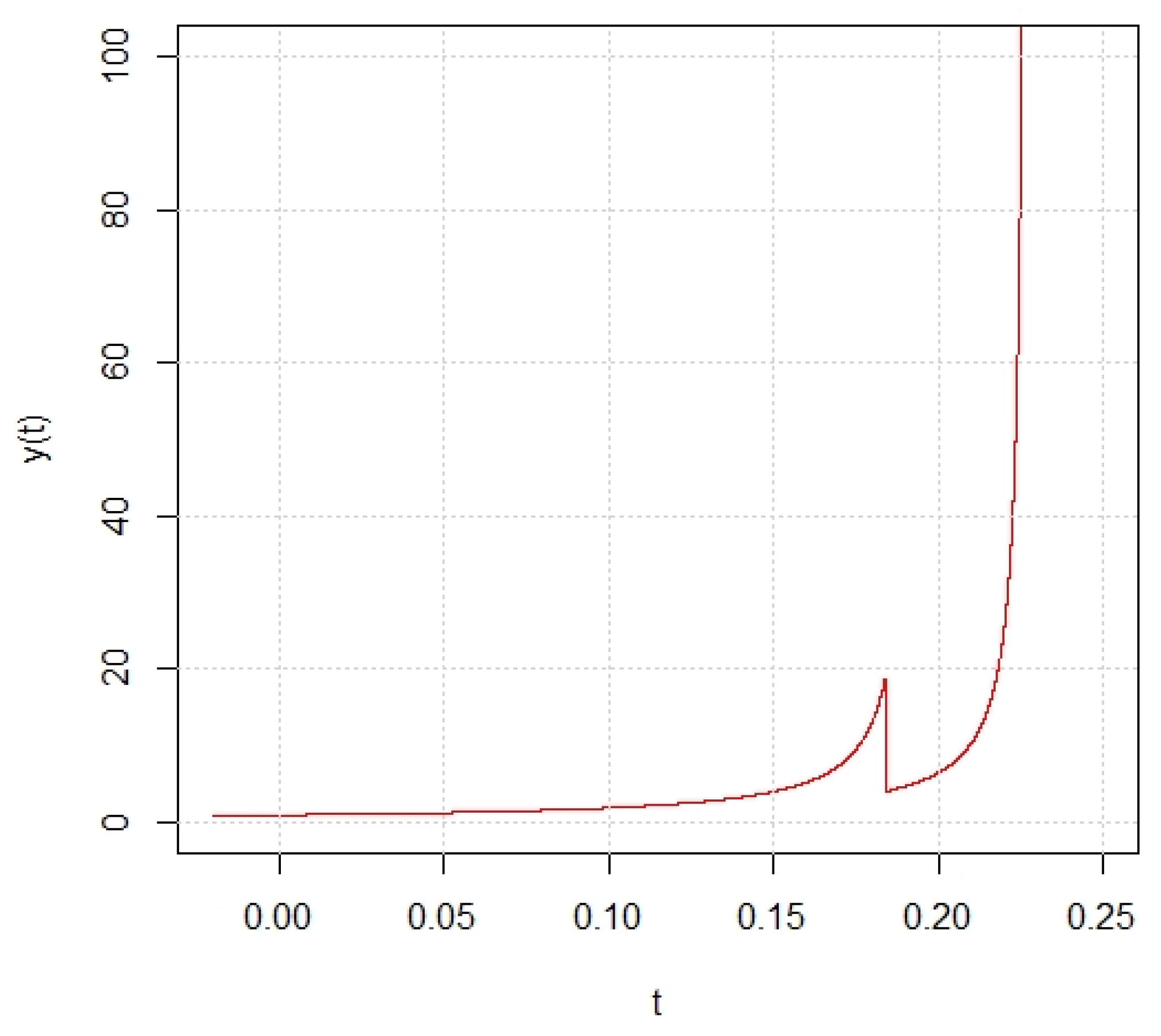
4. A Numeric Example

Next, we will discuss a numeric example to reveal our control theory.

A scalar nonlinear IDDS is concerned,

$$\{\begin{array}{c}dy\left(t\right)=\left[0.5y\left(t\right)+0.1y\left(t-\mu \left(t\right)\right)\right]y\left(t\right)dt,\hspace{0.17em}\hspace{0.17em}\hspace{0.17em}\hspace{0.17em}\hspace{0.17em}\hspace{0.17em}\hspace{0.17em}\hspace{0.17em}\hspace{0.17em}t\ge 0,t\ne {\xi }_g,g=1,2,\cdots \\ y\left({\xi }_g\right)=0.5\left(1-{0.6}^g\right)y\left({\xi }_g-\right)+0.5sin(\left(1-{0.6}^g\right)y\left({\xi }_g-\right))\end{array}\hspace{0.17em}\hspace{0.17em}\hspace{0.17em}\hspace{0.17em}\hspace{0.17em}$$

(5)

where $\mu \left(t\right)=0.01\left(1+cos(t\right))$, ${\xi }_g=0.2g$.

Remark 8.

Essentially, this system is a one-species impulsive population system. The impulsive jump here is the simple combination of linear form and sine form. Thereinto, these parameter values are just to verify our theory.

From the computer simulation (i.e., Figure 1), IDDS (5) explodes to the infinity on a finite instant. Based on our theory, polynomial random noise $\left|y\left(t\right)\right|y\left(t\right)\dot{B}\left(t\right)$ is introduced to suppress its explosive behavior, and the stochastically controlled IDDS becomes

$$\{\begin{array}{c}dy\left(t\right)=\left[0.5y\left(t\right)+0.1y\left(t-\mu \left(t\right)\right)\right]y\left(t\right)dt+\left|y\left(t\right)\right|y\left(t\right)dB\left(t\right)\hspace{0.17em}\hspace{0.17em}\hspace{0.17em}t\ge 0,t\ne {\xi }_g,g=1,2,\cdots ,\\ y\left({\xi }_g\right)=0.5\left(1-{0.6}^g\right)y\left({\xi }_g-\right)+0.5\sin (\left(1-{0.6}^g\right)y\left({\xi }_g-\right))\end{array}$$

(6)

Obviously, SIDDS (6) satisfies Assumptions 1, 2 with $b_g=1-{0.6}^g$, and $\underset{r,L}{max}\prod _{k=r}^L{b}_k{}^2<\infty$ holds. Hence, SIDDS (6) admits a unique global solution by Theorem 1 (see Figure 2). Moreover, SIDDS (6) is bounded by Theorem 2, and grows at most in the polynomial form by Theorem 3 (see Figure 3).

5. Conclusions and Future Discussion

Fortunately, the questions in Section 1 have been well answered. This note illustrates that one polynomial random noise can suppress the explosive behavior of IDDS (1) with Assumptions 1 and 2, and make it grow at most in the polynomial form. Nevertheless, the time-varying delay here is bounded, and nonlinear impulses here need to fulfill Assumptions 2. How to relax these two constraints will be our further work.

References

1. Khasminiskii, R.Z. Stochatic Stability of Differential Equations; Sijthoff and Noordhoff: Alphen aan den Rijn, The Netherlands, 1981. [Google Scholar]
2. Arnold, L.; Crauel, H.; Wihstutz, V. Stabilization of Linear Systems by Noise. SIAM J. Control Optim. 1983, 21, 451–461. [Google Scholar] [CrossRef]
3. Mao, X. Stochastic Differential Equations and Applications; Horwood: Chichester, UK, 1997. [Google Scholar]
4. Mao, X. Exponential Stability of Stochastic Differential Equations; Dekker: New York, NY, USA, 1994. [Google Scholar]
5. Appleby, J.A.D.; Mao, X. Stochatic stabilisation of functional differential equations. Syst. Control Lett. 2005, 54, 1069–1081. [Google Scholar] [CrossRef]
6. Appleby, J.A.D.; Mao, X.; Rodkina, A. Stabilisation and destabilization of nonlinear differential equations by noise. IEEE Trans. Autom. Control 2008, 53, 638–691. [Google Scholar] [CrossRef] [Green Version]
7. Mao, X.; Marion, G.; Renshaw, E. Environmental noise suppresses explosion in population dynamics. Stoch. Processes Appl. 2002, 97, 95–110. [Google Scholar] [CrossRef]
8. Wu, F.; Hu, S. Suppression and stabilization of noise. Int. J. Control 2009, 82, 2150–2157. [Google Scholar] [CrossRef]
9. Wu, F.; Hu, S. Stochastic suppression and stabilization of delay differential systems. Int. J. Robust Nonlinear Control 2011, 21, 488–500. [Google Scholar] [CrossRef]
10. Yin, G.; Zhao, G.; Wu, F. Regularization and Stabilization of Randomly Switching Dynamic Systems. SIAM J. Appl. Math. 2012, 72, 1361–1382. [Google Scholar] [CrossRef]
11. Deng, F.; Luo, Q.; Mao, X. Stochastic stabilization of hybrid differential equations. Automatica 2012, 48, 2321–2328. [Google Scholar] [CrossRef]
12. Huang, L. Stochastic stabilization and destabilization of nonlinear differential equations. Syst. Control Lett. 2013, 62, 163–169. [Google Scholar] [CrossRef]
13. Deng, F.; Luo, Q.; Mao, X.; Pang, S. Noise suppresses or expresses exponential growth. Syst. Control Lett. 2008, 57, 262–270. [Google Scholar] [CrossRef] [Green Version]
14. Hu, G.; Liu, M.; Mao, X.; Song, M. Noise expresses exponential growth under regime switching. Syst. Control Lett. 2009, 58, 691–699. [Google Scholar] [CrossRef] [Green Version]
15. Zhu, S.; Yang, Q.; Shen, Y. Noise further expresses exponential decay for globally exponentially stable time-varying delayed neural networks. Neural Netw. 2016, 77, 7–13. [Google Scholar] [CrossRef] [PubMed]
16. Liu, L.; Shen, Y. Noise suppresses explosive solutions of differential systems with coefficients satisfying the polynomial growth condition. Automatica 2012, 48, 619–624. [Google Scholar] [CrossRef]
17. Feng, L.; Wu, Z.; Zheng, S. A note on explosion suppression for nonlinear delay differential systems by polynomial noise. Int. J. Gen. Syst. 2018, 47, 137–154. [Google Scholar] [CrossRef]
18. Feng, L.; Li, S.; Song, R.; Li, Y. Suppression of explosion by polynomial noise for nonlinear differential systems. Sci. China Inf. Sci. 2018, 61, 136–146. [Google Scholar] [CrossRef]
19. Dubkov, A.A.; Spagnolo, B. Verhulst model with Lévy white noise excitation. Eur. Phys. J. B 2008, 65, 361–367. [Google Scholar] [CrossRef] [Green Version]
20. Spagnolo, B.; Dubkov, A.A.; Pankratov, A.L.; Pankratova, E.V.; Fiasconaro, A.; Ochab-Marcinek, A. Lifetime of metastable states and suppression of noise in interdisciplinary physical models. Acta Phys. Pol. B 2008, 38, 1925–1950. [Google Scholar]
21. Dubkov, A.A.; Litovsky, I.A. Probabilistic characteristics of noisy Van der Pol type oscillator with nonlinear damping. J. Stat. Mech. Theory Exp. 2016, 2016, 054036. [Google Scholar] [CrossRef]
22. Mikhaylov, A.N.; Guseinov, D.V.; Belov, A.I.; Korolev, D.S.; Shishmakova, V.A.; Koryazhkina, M.N.; Filatov, D.O.; Alonso, F.V.; Carollo, A.; Spagnolo, B.; et al. Stochastic resonance in a Metal-Oxide memristive device. Chaos Solitons Fractals 2021, 144, 110723. [Google Scholar] [CrossRef]
23. Lakshmikantham, V.; Bainov, D.D.; Simeonov, P.S. Theory of Impulsive Differential Equations; World Scientific: Singapore, 1989. [Google Scholar]
24. Feketa, P.; Klinshov, V.; Lücken, L. A survey on the modeling of hybrid behaviors: How to account for impulsive jumps properly. Commun. Nonlinear Sci. Numer. Simul. 2021, 103, 105955. [Google Scholar] [CrossRef]
25. Yang, X.; Lu, J.; Ho, D.W.C.; Song, Q. Synchronization of uncertain hybrid switching and impulsive complex networks. Appl. Math. Model. 2018, 59, 379–392. [Google Scholar] [CrossRef]
26. Yang, X.; Li, X.; Lu, J.; Cheng, Z. Synchronization of time-delayed complex networks with switching topology via hybrid actuator fault and impulsive effects control. IEEE Trans. Cybern. 2020, 50, 4043–4052. [Google Scholar] [CrossRef] [PubMed]
27. Zhang, W.; Feng, L.; Wu, Z.; Park, J.H. Stability criteria of random delay differential systems subject to random impulses. Int. J. Robust Nonlinear Control 2021, 31, 6681–6698. [Google Scholar] [CrossRef]
28. Peng, D.; Li, X.; Rakkiyappan, R.; Ding, Y. Stabilization of stochastic delayed systems: Event-triggered impulsive control. Appl. Math. Comput. 2021, 401, 126054. [Google Scholar] [CrossRef]
29. Fu, X.; Li, X. LMI conditions for stability of impulsive stochastic Cohen–Grossberg neural networks with mixed delays. Commun. Nonlinear Sci. Numer. Simul. 2011, 16, 435–454. [Google Scholar] [CrossRef]
30. Hu, W.; Zhu, Q. Stability analysis of impulsive stochastic delayed differential systems with unbounded delays. Syst. Control Lett. 2020, 136, 104606. [Google Scholar] [CrossRef]
31. Peng, S.; Deng, F. New Criteria on pth Moment Input-to-State Stability of Impulsive Stochastic Delayed Differential Systems. IEEE Trans. Autom. Control 2017, 62, 3573–3579. [Google Scholar] [CrossRef]
32. Cheng, P.; Deng, F.; Yao, F. Almost sure exponential stability and stochastic stabilization of stochastic differential systems with impulsive effects. Nonlinear Anal. Hybrid Syst. 2018, 30, 106–117. [Google Scholar] [CrossRef]
33. Hao, S.; Zhang, C.; Feng, L.; Yan, S. Noises for Impulsive Differential Systems. IEEE Access 2019, 7, 138253–138259. [Google Scholar] [CrossRef]
34. Feng, L.; Wu, Z.; Cao, J.; Zheng, S.; Alsaadi, F.E. Exponential stability for nonlinear hybrid stochastic systems with time varying delays of neutral type. Appl. Math. Lett. 2020, 107, 106468. [Google Scholar] [CrossRef]
35. Shukla, A.; Patel, R. Existence and Optimal Control Results for Second-Order Semilinear System in Hilbert Spaces. Circuits Syst. Signal Process. 2021, 40, 4246–4258. [Google Scholar] [CrossRef]
36. Singh, A.; Shukla, A.; Vijayakumar, V.; Udhayakumar, R. Asymptotic stability of fractional order (1,2] stochastic delay differential equations in Banach spaces. Chaos Solitons Fractals 2021, 150, 111095. [Google Scholar] [CrossRef]
Figure 1. Trajectory of IDDS (5) with ζ = 1 . by Euler-Maruyama scheme with step 10 5 .
Mathematics 10 01525 g001
Figure 2. Sample trajectory of SIDDS (6) with ζ = 1 by Euler-Maruyama scheme with step 10 5 .
Mathematics 10 01525 g002
Figure 3. Sample trajectory of l o g ( 1 + | y ( t ) | 2 ) / l o g t for SIDDS (6) by Euler-Maruyama scheme with step 10 5 .
Mathematics 10 01525 g003
Publisher’s Note: MDPI stays neutral with regard to jurisdictional claims in published maps and institutional affiliations.