Tracking Control for Triple-Integrator and Quintuple-Integrator Systems with Single Input Using Zhang Neural Network with Time Delay Caused by Backward Finite-Divided Difference Formulas for Multiple-Order Derivatives

Abstract

Tracking control for multiple-integrator systems is regarded as a fundamental problem associated with nonlinear dynamic systems in the physical and mathematical sciences, with many applications in engineering fields. In this paper, we adopt the Zhang neural network method to solve this nonlinear dynamic problem. In addition, in order to adapt to the requirements of real-world hardware implementations with higher-order precision for this problem, the multiple-order derivatives in the Zhang neural network method are estimated using backward finite-divided difference formulas with quadratic-order precision, thus producing time delays. As such, we name the proposed method the Zhang neural network method with time delay. Moreover, we present five theorems to describe the convergence property of the Zhang neural network method without time delay and the quadratic-order error pattern of the Zhang neural network method with time delay derived from the backward finite-divided difference formulas with quadratic-order precision, which specifically demonstrate the effect of the time delay. Finally, tracking controllers with quadratic-order precision for multiple-integrator systems are constructed using the Zhang neural network method with time delay, and two numerical experiments are presented to substantiate the theoretical results for the Zhang neural network methods with and without time delay.

1. Introduction

In real-world engineering applications, many control systems are characterized by nonlinearity, which are mathematically described as nonlinear dynamic systems [1,2,3]. The problem of tracking control for a given nonlinear system with single input, which focuses on studying their dynamic behaviors, can be formulated as follows [4,5,6,7,8]:

$$\left\{\begin{array}{c}\dot{\mathbf{x}}=\mathbf{f}(\mathbf{x},u,t),\hfill \\ y=h\left(\mathbf{x}\right),\hfill \end{array}\right.$$

(1)

where $\mathbf{x}\in {\mathbb{R}}^n$ is the state vector of the system; $y\in \mathbb{R}$ and $u\in \mathbb{R}$ are the output and control input of the system, respectively; and $y_{\mathrm{d}}$ is the desired path. The target of the above tracking control problem for a given nonlinear system with single input is to make the tracking error $e_{\mathrm{tr}}=y-y_{\mathrm{d}}$ equal to zero for a suitable initial state. In particular, multiple-integrator (MI) systems are usually considered as fundamental nonlinear dynamic systems in the physical and mathematical sciences, having many applications in the engineering fields [9,10], such as secure communication [11,12,13], electrical engineering [14], and economics [15]. Moreover, the tracking control of MI systems has contributed significantly to their real-world implementation and has attracted a lot of attention in related fields [16,17,18,19].

Some methods/algorithms which construct a controller to track the desired path $y_{\mathrm{d}}\left(t\right)$ accurately have been designed to address the tracking control problem for MI systems [20,21,22,23,24,25,26,27,28,29,30,31]. These methods/algorithms mainly include the input–output linearization (IOL) method [21], variants of the IOL method (e.g., approximate IOL, a switching scheme of approximate IOL, and exact IOL) [22,23,24], and neural network-based dynamic methods [25,26,27,28,29,30,31]. The IOL method and its variants are usually adopted to tackle the problem of tracking control for nonlinear systems; however, they always face problems related to singularities and instability at some key points, causing the nonlinear system to fall outside of a well-defined relative degree. Thus, more than two controllers with single linear output should generally be constructed, which increases the complexity of the corresponding algorithms [23,24]. Therefore, neural network-based dynamic methods have been adopted to tackle with the problem of tracking control for nonlinear systems, due to their high-speed parallel-distributed processing properties [32,33,34,35,36,37,38,39].

As an effective approach in the neural network-based dynamic methods category, the Zhang neural network (ZNN) has been proposed to deal with the problem of tracking control for nonlinear dynamic systems. In [32,33], Zhang et al. addressed the problems of tracking control for the Lu chaotic (LC) system with multiple additive inputs and a double-integrator (DI) system with linear and nonlinear outputs by combining the ZNN and the gradient dynamics (GD) method. In [34], Zhang et al. proposed a variant of the ZNN approach to tackle the singularity-conquering problem in tracking control for the single-input LC system and the mixed inputs modified Lorenz chaotic system. In [40], Zhang et al. developed a method, named Zhang gradient control (ZGC), to solve an MI system with linear and nonlinear outputs. In [41], Jin et al. derived a group of controllers based on the ZGC method for a modified Lorenz chaotic system with an additive input or a mixture of additive and multiplicative inputs. In [42], Li et al. developed a group of effective controllers using the zeroing dynamics (ZD) method, which is related to the ZNN method, in order to tackle the synchronization problem of the chaotic system by considering model uncertainty, parameter perturbation, and external noise disturbance. In [43], Huang et al. proposed a method using the ZNN method and the three-step Zhang et al. discretization (i.e., ZeaD) formulas at four points to solve the synchronization problem of discrete LC system with a single input. In [44], Ling et al. presented a group of controllers based on the ZNN method to solve the synchronization problem of the Genesio Chaotic (GC) system with or without noise disturbance. In [45], Zhang et al. developed a generalized Zhang equivalency (ZE), also related to the ZNN method, in order to revisit the problem of tracking control for the single additive input LC system. In [46], Li et al. constructed a type of ZNN-based controller to track MI systems with noise disturbance.

The above studies have verified the effectiveness and accuracy of ZNN methods. For the controllers that were constructed using ZNN-based methods, the derivatives employed in the design process, such as ${\dot{y}}_{\mathrm{d}}\left(t\right)$, ${\ddot{y}}_{\mathrm{d}}\left(t\right)$, ${\stackrel{⃛}{y}}_{\mathrm{d}}\left(t\right)$, and ${\stackrel{⃜}{y}}_{\mathrm{d}}\left(t\right)$, are often computed directly using accurate derivative formulas; thus, the problem of tracking control for MI systems with high accuracy can be achieved in the case with no time delay. However, as is well-known, time delays always appear in real-world applications, especially with the implementation of different types of neural networks [47,48,49,50,51,52,53,54,55,56,57,58,59,60,61]. For instance, in [48], Stamov et al. studied the stability problem of Bidirectional Associative Memory (BAM) Cohen–Grossberg-type impulsive neural networks with time-varying delays by using manifold notions. In [49], Chanthorn et al. reported the robust dissipativity of Hopfield-type complex-valued neural network models incorporated with time-varying delays and linear fractional uncertainties using the multiple integral inequality method. In the same year, Chanthorn et al. presented the robust stability of complex-valued stochastic neural networks with time-varying delays and parameter uncertainties by exploiting the real–imaginary separate-type activation function [50]. In [55], Akhmet et al. studied the unpredictable oscillations problem in Hopfield-type neural networks with time delay and advanced arguments that can be applied to neuroscience. In [56], Rajchakit et al. studied the finite-time synchronization problem of Clifford-valued neural networks with finite-time distributed delays using the number field transformation method. In [61], Sun and Liu presented an adaptive synchronization control and synchronization-based parameter identification method for fractional chaotic neural networks with time-varying delays. Although the above mentioned research works studied the stability properties of the control problem for different neural network systems with time-varying delay, they did not attempt to understand the effect of time delay in the controller design procedure for different nonlinear dynamic systems. As a canonical type of neural network, the influence of time delay caused by approximating the derivatives in the ZNN method needs to be studied, in order to deal with the problem of tracking control for nonlinear systems. In our previous work [62], we have investigated ZNN methods without time delay and the first-order error pattern of ZNN methods with time delay derived from the backward finite-divided difference rules with linear-order precision. However, higher-order precision tracking controllers for nonlinear systems constructed based on ZNN methods with time delay should be developed, in order to satisfy the demands of real-world engineering applications.

In this paper, the multiple-order derivatives in the ZNN method are estimated using backward finite-divided difference formulas (BFDDFs) with quadratic-order precision, which produce time delays; as such, we call the proposed method the order-N ZNN method with time delay. To check the validity and precision of the order-N ZNN method with time delay, in terms of solving the problem of tracking control for nonlinear systems, both theoretical results and systematic proofs are presented. In addition, numerical experiments considering the problem of tracking control for a triple-integrator (TI) system with non-linear output function (NOF) and a quintuple-integrator (QI) system with linear output function (LOF) are conducted, in order to substantiate the theoretical results of the order-N ZNN methods with and without time delay.

The remainder of this paper is organized into four sections, and the main contents are illustrated in Figure 1. Section 2 presents five theorems for order-N ZNN methods with and without time delay. Section 3 investigates the problem of tracking control for a TI system with NOF. Numerical experiments substantiate the theoretical results of order-N ZNN methods with and without time delay. Section 4 investigates the problem of tracking control for the QI system with LOF. Again, numerical experiments substantiate the theoretical results of order-N ZNN methods with and without time delay. Finally, in Section 5, we present the conclusion of this paper. The contributions of our study can be summarized as follows:

• To study the impact of the time delay caused by the multiple-order derivative approximation on the order-N ZNN method. To investigate this, the order-N ZNN model is transformed into a non-homogeneous time delay differential equation by using BFDDFs with quadratic-order precision.
• Five theorems, together with rigorous mathematical proofs, are illustrated to describe the convergence properties of the order-N ZNN method without time delay and the quadratic-order error pattern of the order-N ZNN method with time delay derived from the backward finite-divided difference formulas with quadratic-order precision, which specifically demonstrate the effect of the time delay.
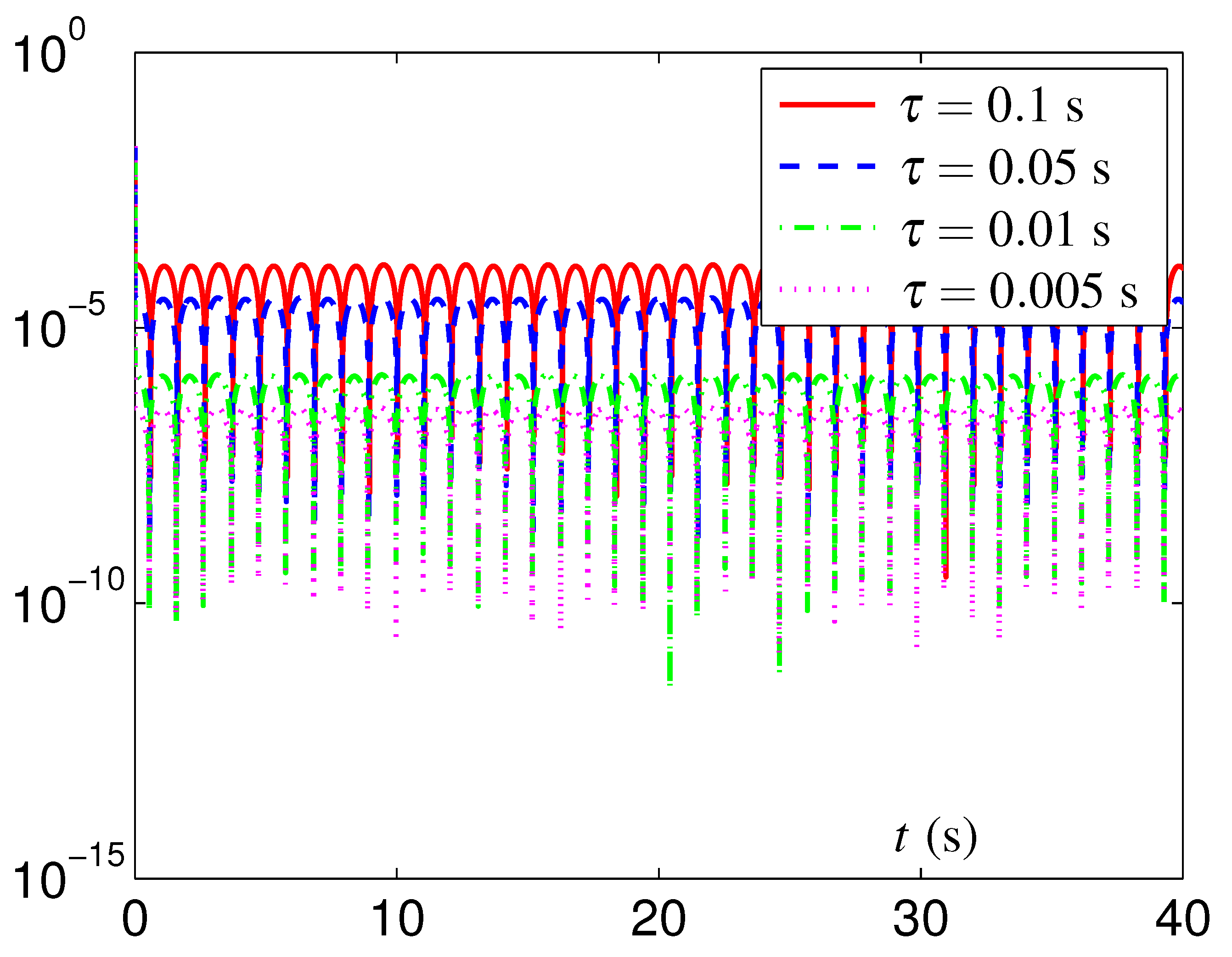
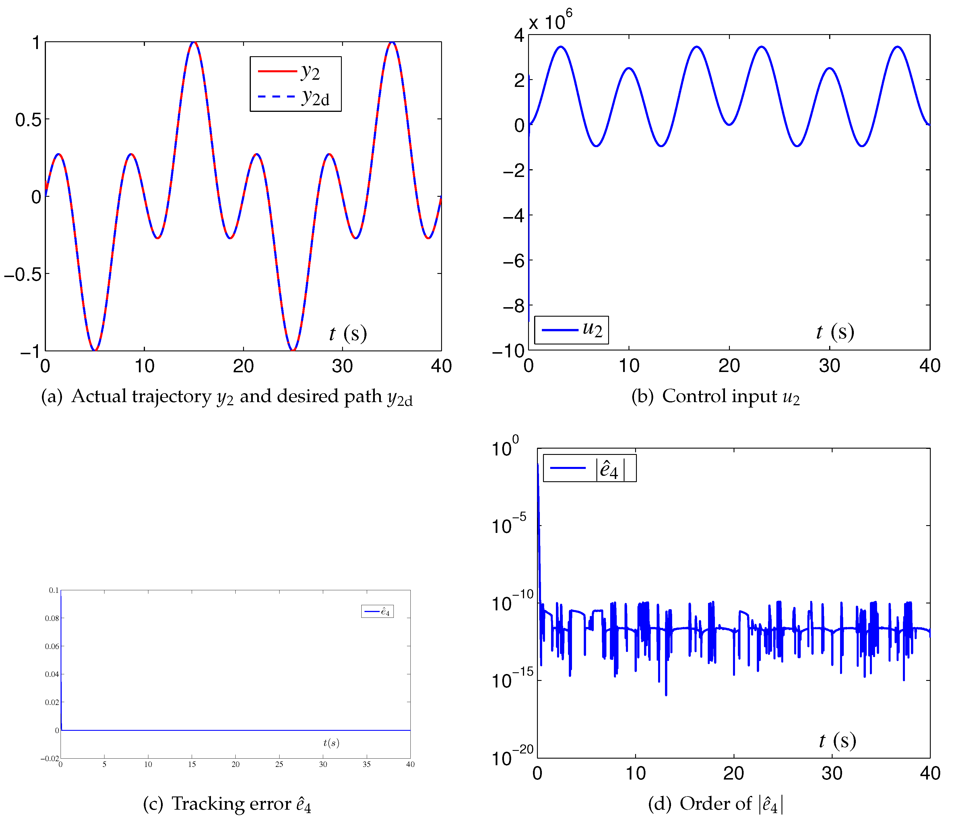
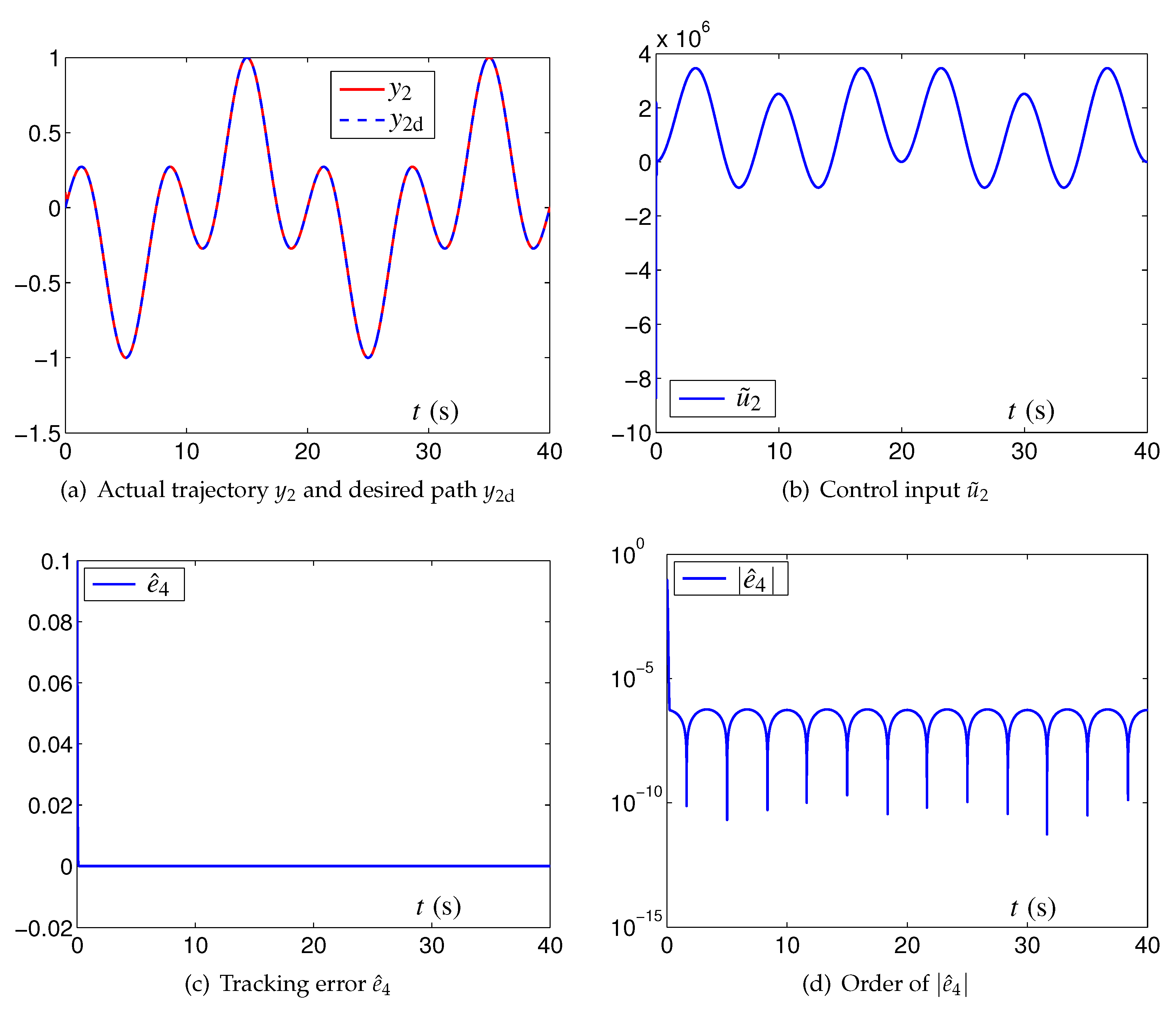
• The ZNN method with time delay is successfully adopted to solve the problem of tracking control for the TI system with NOF and the QI system with LOF, and the corresponding numerical experiment results substantiate the quadratic-order error pattern of order-N ZNN methods with time delay derived from the backward finite-divided difference formulas with quadratic-order precision.

2. Multiple-Order ZNN Methods with and without Time Delay

In this section, the backward finite-divided difference formulas are revisited, as a method for approximating derivatives of various orders for target functions. Based on the uniform order of truncation errors for backward finite-divided difference formulas, the multiple-order ZNN methods with and without time delay are developed, and we provide five theorems about the order-N ZNN methods with and without time delay, together with theoretical proofs.

2.1. Backward Finite-Divided Difference Formulas

As mentioned in the introduction, time delays always appear in the real-world applications. In particular, as the time-dependent states of a system may be measured using sensors, or produced by complex transformations including Fourier and Laplace transforms, among others, their derivatives are difficult to obtain directly. To address this, we adopt the BFDDFs, which only need historical states to approximate the derivatives, which leads to multiple-step time delay. BFDDFs computed by the Lagrange interpolation polynomial play an important role in theoretical analyses and numerical experiments. For convenience, we list several BFDDFs and their corresponding truncation errors in the following

Table 1. Backward finite-divided difference formulas for order-n derivative functions.

Order-n Derivative Function	Backward Finite-Divided Difference Formula	Truncation Error
$\dot{z}\left(t\right)$	$\left(3z\right(t)-4z(t-\tau )+z(t-2\tau \left)\right)/2\tau$	$O\left({\tau }^2\right)$
$\ddot{z}\left(t\right)$	$(2z\left(t\right)-5z(t-\tau )+4z(t-2\tau )-z(t-3\tau ))/{\tau }^2$	$O\left({\tau }^2\right)$
$\stackrel{⃛}{z}\left(t\right)$	$(5z\left(t\right)-18z(t-\tau )+24z(t-2\tau )-14z(t-3\tau )+3z(t-4\tau ))/2{\tau }^3$	$O\left({\tau }^2\right)$
$\stackrel{⃜}{z}\left(t\right)$	$(3z\left(t\right)-14z(t-\tau )+26z(t-2\tau )-24z(t-3\tau )+11z(t-4\tau )-2z(t-5\tau ))/{\tau }^4$	$O\left({\tau }^2\right)$

, where $z\left(t\right)$ is a desired function or a desired time-continuous matrix, and $\tau$ is the sampling time delay. Specifically, we use the formulas in Table 1 to construct the controller for MI systems with a single input and investigate the effect of time delay in the ZNN method. We believe that other BFDDFs with uniform-order truncation error can also be adopted to construct controllers for nonlinear system with single input.

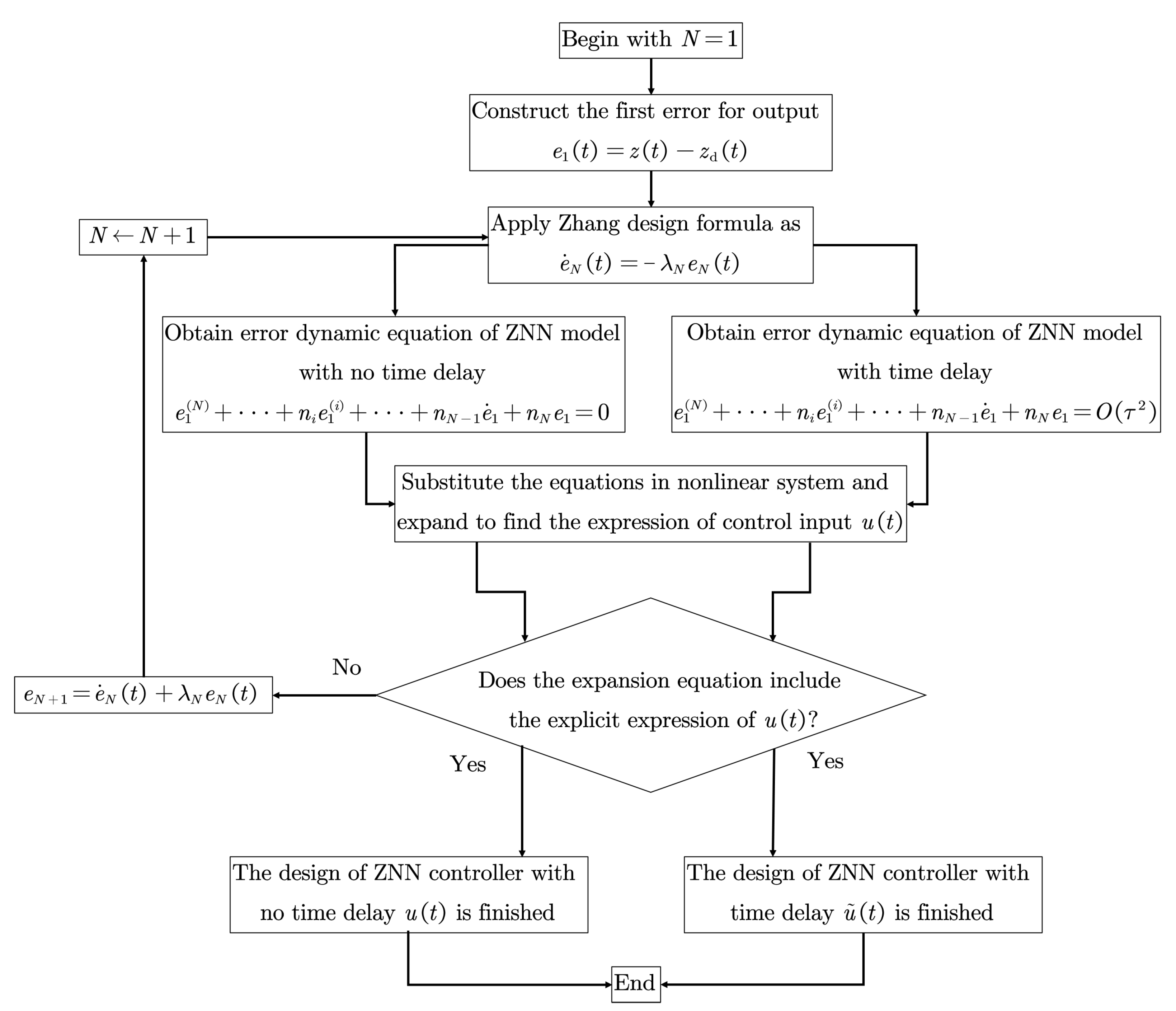
2.2. Order-N ZNN Methods with and without Time Delay

In order to solve the problem of tracking control for nonlinear systems and to optimize the solution to other real-world problems, the order-N ZNN methods with and without time delay are constructed step-by-step in this subsection.

To construct the ZNN method, the error function $e_1$ captured from the actual trajectory and the desired path is formulated as

$$e_1=z-z_{\mathrm{d}},$$

(2)

where z is the actual trajectory of the nonlinear system and $z_{\mathrm{d}}$ is the desired path. Then, the ZNN design formula [25,29,30,31] is adopted as

$${\dot{e}}_1=-{\lambda }_1{e}_1,$$

(3)

where ${\lambda }_1>0\in \mathbb{R}$ is the ZNN design parameter, which is adopted to control the convergence rate of ZNN solution [25,29]. Equation (3) is reformulated as the corresponding standard form ${\dot{e}}_1+{\lambda }_1{e}_1=0$, which is the so-called order-1 ZNN model without time delay. However, when the order-1 ZNN model without time delay is approximated using the BFDDFs given in Table 1, it has a truncation error of $O\left({\tau }^2\right)$. Therefore, the order-1 ZNN model without time delay is formulated into the following order-1 ZNN model with time delay:

$${\dot{e}}_1+{\lambda }_1{e}_1=O\left({\tau }^2\right).$$

(4)

In addressing the problem of tracking control for MI systems, one needs to use the ZNN method several times to design suitable controllers; that is, one must use the ZNN design formula to construct an order-N ZNN model without time delay and with time delay, as follows. Let $e_2$ denote the second error function, which is represented using a linear combination of $e_1$ and its derivative ${\dot{e}}_1$, in the without time delay case, as

$$e_2={\dot{e}}_1+{\lambda }_1{e}_1.$$

(5)

The ZNN design formula is adopted again for the second error function $e_2$,

$${\dot{e}}_2=-{\lambda }_2{e}_2,$$

(6)

where ${\lambda }_2>0\in \mathbb{R}$ is the ZNN design parameter. Substituting Equation (5) into Equation (6), one obtains the following order-2 ZNN model without time delay, which is described by a constant coefficient homogeneous linear ordinary differential equation of order 2:

$${\ddot{e}}_1+({\lambda }_1+{\lambda }_2){\dot{e}}_1+{\lambda }_1{\lambda }_2{e}_1=0.$$

(7)

When the order-2 ZNN model without time delay is approximated by the BFDDFs mentioned in Table 1, one obtains the following order-2 ZNN model with time delay:

$${\ddot{e}}_1+({\lambda }_1+{\lambda }_2){\dot{e}}_1+{\lambda }_1{\lambda }_2{e}_1=O\left({\tau }^2\right).$$

(8)

Let $e_3$ denote the third error function, which is represented using a linear combination of $e_2$ and its derivative ${\dot{e}}_2$, in the without time delay case, as

$$e_3={\dot{e}}_2+{\lambda }_2{e}_2.$$

(9)

Substituting Equation (5) into Equation (9), one obtains the following relation between $e_3$ and $e_1$:

$$e_3={\ddot{e}}_1+({\lambda }_1+{\lambda }_2){\dot{e}}_1+{\lambda }_1{\lambda }_2{e}_1.$$

(10)

The ZNN design formula is used again for the third error function $e_3$,

$${\dot{e}}_3=-{\lambda }_3{e}_3,$$

(11)

where ${\lambda }_3>0\in \mathbb{R}$ is the ZNN design parameter. By substituting Equation (10) into Equation (11), one obtains the order-3 ZNN model without time delay, as follows:

$${\stackrel{⃛}{e}}_1+({\lambda }_1+{\lambda }_2+{\lambda }_3){\ddot{e}}_1+({\lambda }_1{\lambda }_2+{\lambda }_2{\lambda }_3+{\lambda }_1{\lambda }_3){\dot{e}}_1+{\lambda }_1{\lambda }_2{\lambda }_3{e}_1=0.$$

(12)

When the order-3 ZNN model without time delay is approximated by the BFDDFs mentioned in Table 1, one obtains the following order-3 ZNN model with time delay:

$${\stackrel{⃛}{e}}_1+({\lambda }_1+{\lambda }_2+{\lambda }_3){\ddot{e}}_1+({\lambda }_1{\lambda }_2+{\lambda }_2{\lambda }_3+{\lambda }_1{\lambda }_3){\dot{e}}_1+{\lambda }_1{\lambda }_2{\lambda }_3{e}_1=O\left({\tau }^2\right).$$

(13)

Let $e_4$ denote the forth error function. The relation between the error function $e_4$ and $e_3$, in the without time delay case, is formulated as follows:

$$e_4={\dot{e}}_3+{\lambda }_3{e}_3.$$

(14)

Substituting Equation (10) into Equation (14), one can express the error function $e_4$ as the following linear combination of different order derivatives of $e_1$:

$$e_4={\stackrel{⃛}{e}}_1+({\lambda }_1+{\lambda }_2+{\lambda }_3){\ddot{e}}_1+({\lambda }_1{\lambda }_2+{\lambda }_2{\lambda }_3+{\lambda }_1{\lambda }_3){\dot{e}}_1+{\lambda }_1{\lambda }_2{\lambda }_3{e}_1.$$

(15)

One uses the ZNN design formula for the forth error function $e_4$,

$${\dot{e}}_4=-{\lambda }_4{e}_4,$$

(16)

where ${\lambda }_4>0\in \mathbb{R}$ is the ZNN design parameter. Then, one obtains the following order-4 ZNN model without time delay, as follows:

$${\stackrel{⃜}{e}}_1+m_1{\stackrel{⃛}{e}}_1+m_2{\ddot{e}}_1+m_3{\dot{e}}_1+m_4{e}_1=0,$$

(17)

where $m_1={\lambda }_1+{\lambda }_2+{\lambda }_3+{\lambda }_4$, $m_2={\lambda }_1{\lambda }_2+{\lambda }_1{\lambda }_3+{\lambda }_1{\lambda }_4+{\lambda }_2{\lambda }_3+{\lambda }_2{\lambda }_4+{\lambda }_3{\lambda }_4$, $m_3={\lambda }_1{\lambda }_2{\lambda }_3+{\lambda }_1{\lambda }_2{\lambda }_4+{\lambda }_1{\lambda }_3{\lambda }_4+{\lambda }_2{\lambda }_3{\lambda }_4$, and $m_4={\lambda }_1{\lambda }_2{\lambda }_3{\lambda }_4$. When the order-4 ZNN model without time delay is approximated by the BFDDFs mentioned in Table 1, one obtains the following order-4 ZNN model with time delay:

$${\stackrel{⃜}{e}}_1+m_1{\stackrel{⃛}{e}}_1+m_2{\ddot{e}}_1+m_3{\dot{e}}_1+m_4{e}_1=O\left({\tau }^2\right).$$

(18)

Generally, the $N^{\mathrm{th}}$ error function $e_N$ is defined by the following linear combination of the ${(N-1)}^{\mathrm{th}}$-order function $e_{N-1}$ and its first derivative:

$$e_N={\dot{e}}_{N-1}+{\lambda }_{N-1}{e}_{N-1}.$$

(19)

The ZNN design formula is adopted for the error function $e_N$,

$${\dot{e}}_N=-{\lambda }_N{e}_N,$$

(20)

where ${\lambda }_N>0\in \mathbb{R}$ is the ZNN design parameter. By expressing the $N^{\mathrm{th}}$ error function $e_N$ as the linear combination of the error function $e_1$ and its derivatives with the highest order N, one obtains the following order-N ZNN model without time delay:

$$e_1^{\left(N\right)}+n_1{e}_1^{(N-1)}+···+n_i{e}_1^{\left(i\right)}+···+n_{N-1}{\dot{e}}_1+n_N{e}_1=0,$$

(21)

where $e_1^{\left(i\right)}$ is the $i^{\mathrm{th}}$-order derivative of the error function $e_1$, and the coefficient of corresponding high-order derivative is given by $n_i={\sum }_{1\le l_1<l_2<···<l_i\le n}{\lambda }_{l_1}{\lambda }_{l_2}···{\lambda }_{l_i}$, with Card $\{l_1,l_2,···,l_i\}=i$. Assuming that each order derivative of the desired path can be approximated using BFDDFs with truncation error $O\left({\tau }^2\right)$, one obtains the order-N ZNN model with time delay:

$$e_1^{\left(N\right)}+n_1{e}_1^{(N-1)}+···+n_i{e}_1^{\left(i\right)}+···+n_{N-1}{\dot{e}}_1+n_N{e}_1=O\left({\tau }^2\right).$$

(22)

For better illustration and understanding, in Figure 2, we present a flowchart of the controller design using the ZNN methods with and without time delay for the tracking control of a nonlinear system with single input.

2.3. Error Analysis of Order-N ZNN Methods with and without Time Delay

In this subsection, we introduce five theorems to describe the error properties of the order-N ZNN methods with and without time delay.

Theorem 1.

Assume that there exists a group of backward finite-divided difference formulas with truncation error $O\left({\tau }^2\right)$. As the time t becomes large enough (i.e., $t\gg 0$), the relation between the solution error $e_1\left(t\right)$ of the order-1 ZNN model with time delay (4) and the truncation error $O\left({\tau }^2\right)$ is formulated as $e_1\left(t\right)\approx O\left({\tau }^2\right)/{\lambda }_1=O\left({\tau }^2\right)$, where ${\lambda }_1$ is the ZNN design parameter. In other words, the steady-state solution error $e_1\left(t\right)$ has a positive proportional relationship with the truncation error $O\left({\tau }^2\right)$.

Proof of Theorem 1. 

The order-1 ZNN model with time delay is a non-homogeneous linear differential Equation (4), as follows:

$${\dot{e}}_1+{\lambda }_1{e}_1=O\left({\tau }^2\right).$$

According to the solution structure of non-homogeneous linear ordinary differential equations [63,64], the solution of (4) is expressed as the summation of a special solution of it and the general solution of its corresponding homogeneous equation. Thus, the solution to (4) is given as follows:

$$e_1\left(t\right)=C_{1}exp(-{\lambda }_{1}t)+exp(-{\lambda }_{1}t){\int }_0^{t}O\left({\tau }^2\right)exp\left({\lambda }_1\iota \right)d\iota =C_{1}exp(-{\lambda }_{1}t)+O\left({\tau }^2\right)/{\lambda }_1,$$

where the constant $C_1=e_1\left(0\right)-O\left({\tau }^2\right)/{\lambda }_1$ is computed at the initial time point $t=0$. When $t\to +\infty$, the first term of the above solution $(e_1\left(0\right)-O\left({\tau }^2\right)/{\lambda }_1)exp(-{\lambda }_{1}t)$ approaches zero. Then, as $t\to +\infty$, the first error function is approximated as

$$e_1\left(t\right)\approx O\left({\tau }^2\right)/{\lambda }_1=O\left({\tau }^2\right).$$

The proof is completed. □

Theorem 2.

Assume that there exists a group of backward finite-divided difference formulas with truncation error $O\left({\tau }^2\right)$. As the time t becomes large enough (i.e., $t\gg 0$), the relation between the solution error $e_1\left(t\right)$ of the order-2 ZNN model with time delay (8) and the truncation error $O\left({\tau }^2\right)$ is formulated as $e_1\left(t\right)\approx O\left({\tau }^2\right)/\left({\lambda }_1{\lambda }_2\right)=O\left({\tau }^2\right)$, where ${\lambda }_1$ and ${\lambda }_2$ are the ZNN design parameters. In other words, the steady-state solution error $e_1\left(t\right)$ has a positive proportional relationship with the truncation error $O\left({\tau }^2\right)$.

Proof of Theorem 2. 

The order-2 ZNN model with time delay is a non-homogeneous linear differential equation with constant coefficients (8), as follows:

$${\ddot{e}}_1+({\lambda }_1+{\lambda }_2){\dot{e}}_1+{\lambda }_1{\lambda }_2{e}_1=O\left({\tau }^2\right).$$

The corresponding homogeneous linear differential equation of (8), that is also the order-2 ZNN model without time delay (7), is formulated by setting the free term to zero, as follows:

$${\ddot{e}}_1+({\lambda }_1+{\lambda }_2){\dot{e}}_1+{\lambda }_1{\lambda }_2{e}_1=0,$$

and its characteristic equation is the following algebraic equation:

$$p^2+({\lambda }_1+{\lambda }_2)p+{\lambda }_1{\lambda }_2=0.$$

(23)

The corresponding characteristic roots of (23) are $p_1=-{\lambda }_1$ and $p_2=-{\lambda }_2$. According to the solution structure of non-homogeneous linear ordinary differential equations [63,64], the solution of (8) is expressed as the summation of its special solution and the general solution of its corresponding homogeneous equation. As the free term of (8) can be rewritten as $O\left({\tau }^2\right)=O\left({\tau }^2\right)exp(0·t)$, and the characteristic roots of (7) satisfy $p_1=-{\lambda }_1<0,p_2=-{\lambda }_2<0$, the special solution of (8) is assumed to be of the form $C_{2}exp(0·t)$, which is equal to the constant $C_2$. Substituting $C_2$ into the equation (8), one obtains the following relation:

$${\lambda }_1{\lambda }_2{C}_2=O\left({\tau }^2\right);$$

that is, $C_2=O\left({\tau }^2\right)/{\lambda }_1{\lambda }_2$. As there are two characteristic roots when solving Equation (23), the general solution of (8) is associated with the relationship between ${\lambda }_1$ and ${\lambda }_2$.

Case I If ${\lambda }_1={\lambda }_2$, the general solution of the order-2 ZNN model without time delay is ${\tilde{e}}_1\left(t\right)=(c_1+c_{2}t)exp(-{\lambda }_{1}t)$. Then, the general solution of the order-2 ZNN model with time delay is given by the following function:

$$e_1\left(t\right)=(c_1+c_{2}t)exp(-{\lambda }_{1}t)+O\left({\tau }^2\right)/{\lambda }_1{\lambda }_2.$$

(24)

Case II If ${\lambda }_1\ne {\lambda }_2$, the general solution of the order-2 ZNN model without time delay is ${\tilde{e}}_1\left(t\right)=c_{1}exp(-{\lambda }_{1}t)+c_{2}exp(-{\lambda }_{2}t)$. Then, the general solution of the order-2 ZNN model with time delay is given by the following function:

$$e_1\left(t\right)=c_{1}exp(-{\lambda }_{1}t)+c_{2}exp(-{\lambda }_{2}t)+O\left({\tau }^2\right)/{\lambda }_1{\lambda }_2.$$

(25)

When $t\to +\infty$, both the first term $(c_1+c_{2}t)exp(-{\lambda }_{1}t)$ of function (24) and the first term $c_{1}exp(-{\lambda }_{1}t)+c_{2}exp(-{\lambda }_{2}t)$ of function (25) approach zero. Hence, as $t\to +\infty$, the first error function can be approximated as

$$e_1\left(t\right)\approx O\left({\tau }^2\right)/{\lambda }_1{\lambda }_2=O\left({\tau }^2\right).$$

The proof is completed. □

Theorem 3.

Assume that there exists a group of backward finite-divided difference formulas with truncation error $O\left({\tau }^2\right)$. As the time t becomes large enough (i.e., $t\gg 0$), the relation between the solution error $e_1\left(t\right)$ of the order-3 ZNN model with time delay (13) and the truncation error $O\left({\tau }^2\right)$ is formulated as $e_1\left(t\right)\approx O\left({\tau }^2\right)/\left({\lambda }_1{\lambda }_2{\lambda }_3\right)=O\left({\tau }^2\right)$, where ${\lambda }_1$, ${\lambda }_2$, and ${\lambda }_3$ are the ZNN design parameters. In other words, the steady-state solution error $e_1\left(t\right)$ has a positive proportional relationship with the truncation error $O\left({\tau }^2\right)$.

Proof of Theorem 3. 

The order-3 ZNN model with time delay is a constant coefficient non-homogeneous linear differential Equation (13), as follows:

$${\stackrel{⃛}{e}}_1+({\lambda }_1+{\lambda }_2+{\lambda }_3){\ddot{e}}_1+({\lambda }_1{\lambda }_2+{\lambda }_2{\lambda }_3+{\lambda }_1{\lambda }_3){\dot{e}}_1+{\lambda }_1{\lambda }_2{\lambda }_3{e}_1=O\left({\tau }^2\right).$$

The corresponding homogeneous linear differential equation of (13), which is the order-3 ZNN model without time delay (12), is formulated by setting the free term to zero, as follows:

$${\stackrel{⃛}{e}}_1+({\lambda }_1+{\lambda }_2+{\lambda }_3){\ddot{e}}_1+({\lambda }_1{\lambda }_2+{\lambda }_2{\lambda }_3+{\lambda }_1{\lambda }_3){\dot{e}}_1+{\lambda }_1{\lambda }_2{\lambda }_3{e}_1=0,$$

and its corresponding characteristic function is the following polynomial equation with degree 3:

$$p^3+({\lambda }_1+{\lambda }_2+{\lambda }_3)p^2+({\lambda }_1{\lambda }_2+{\lambda }_2{\lambda }_3+{\lambda }_1{\lambda }_3)p+{\lambda }_1{\lambda }_2{\lambda }_3=0.$$

(26)

Then, the corresponding characteristic roots of (26) are $p_1=-{\lambda }_1$, $p_2=-{\lambda }_2$, and $p_3=-{\lambda }_3$. According to the solution structure of non-homogeneous linear ordinary differential equations [63,64], the solution of (13) is expressed as the summation of its special solution and the general solution of its corresponding homogeneous equation. As the free term of (13) can be rewritten as $O\left({\tau }^2\right)=O\left({\tau }^2\right)exp(0·t)$, and the characteristic roots of (12) satisfy $p_1=-{\lambda }_1<0,p_2=-{\lambda }_2<0,p_3=-{\lambda }_3<0$, the special solution of (13) is assumed to be of the form $C_{3}exp(0·t)$, which is equal to the constant $C_3$. Substituting $C_3$ into Equation (13), one obtains the following relation:

$${\lambda }_1{\lambda }_2{\lambda }_3{C}_3=O\left({\tau }^2\right);$$

that is, $C_3=O\left({\tau }^2\right)/{\lambda }_1{\lambda }_2{\lambda }_3$. Since there are three characteristic roots by solving Equation (26), the general solution of (13) is associated with the relationship between ${\lambda }_1$, ${\lambda }_2$, and ${\lambda }_3$.

Case I If ${\lambda }_1={\lambda }_2={\lambda }_3$, the general solution of the order-3 ZNN model without time delay is ${\tilde{e}}_1\left(t\right)=(c_1+c_{2}t+c_3{t}^2)exp(-{\lambda }_{1}t)$. Then, the general solution of the order-3 ZNN model with time delay is given by the following function:

$$e_1\left(t\right)=(c_1+c_{2}t+c_3{t}^2)exp(-{\lambda }_{1}t)+O\left({\tau }^2\right)/{\lambda }_1{\lambda }_2{\lambda }_3.$$

(27)

Case II If there are exactly two equal characteristic roots of (12) (without loss of generality, we assume $p_1=p_2\ne p_3$), the general solution of the order-3 ZNN model without time delay is ${\tilde{e}}_1\left(t\right)=(c_1+c_{2}t)exp(-{\lambda }_{1}t)+c_{3}exp(-{\lambda }_{3}t)$. Then, the general solution of the order-3 ZNN model with time delay is given by the following function:

$$e_1\left(t\right)=(c_1+c_{2}t)exp(-{\lambda }_{1}t)+c_{3}exp(-{\lambda }_{3}t)+O\left({\tau }^2\right)/{\lambda }_1{\lambda }_2{\lambda }_3.$$

(28)

Case III If the three characteristic roots of (12) mutually differ, the general solution of the order-3 ZNN model without time delay is ${\tilde{e}}_1\left(t\right)=c_{1}exp(-{\lambda }_{1}t)+c_{2}exp(-{\lambda }_{1}t)+c_{3}exp(-{\lambda }_{3}t)$. Then, the general solution of the order-3 ZNN model with time delay is given by the following function:

$$e_1\left(t\right)=c_{1}exp(-{\lambda }_{1}t)+c_{2}exp(-{\lambda }_{1}t)+c_{3}exp(-{\lambda }_{3}t)+O\left({\tau }^2\right)/{\lambda }_1{\lambda }_2{\lambda }_3.$$

(29)

When $t\to +\infty$, the first term $(c_1+c_{2}t+c_3{t}^2)exp(-{\lambda }_{1}t)$ of function (27), the first term $(c_1+c_{2}t)exp(-{\lambda }_{1}t)+c_{3}exp(-{\lambda }_{3}t)$ of function (28), and the first term $c_{1}exp(-{\lambda }_{1}t)+c_{2}exp(-{\lambda }_{1}t)+c_{3}exp(-{\lambda }_{3}t)$ of function (29) approach zero. Hence, as $t\to +\infty$, the first error function can be approximated as

$$e_1\left(t\right)\approx O\left({\tau }^2\right)/{\lambda }_1{\lambda }_2{\lambda }_3=O\left({\tau }^2\right).$$

(30)

The proof is completed. □

Theorem 4.

Assume that there exists a group of backward finite-divided difference formulas with truncation error $O\left({\tau }^2\right)$. As the time t becomes large enough (i.e., $t\gg 0$), the relation between the solution error $e_1\left(t\right)$ of the order-4 ZNN model with time delay (18) and the truncation error $O\left({\tau }^2\right)$ is formulated as $e_1\left(t\right)\approx O\left({\tau }^2\right)/\left({\lambda }_1{\lambda }_2{\lambda }_3{\lambda }_4\right)=O\left({\tau }^2\right)$, where ${\lambda }_1$, ${\lambda }_2$, ${\lambda }_3$, and ${\lambda }_4$ are the ZNN design parameters. In other words, the steady-state solution error $e_1\left(t\right)$ has a positive proportional relationship with the truncation error $O\left({\tau }^2\right)$.

Proof of Theorem 4. 

The order-4 ZNN model with time delay is a constant coefficient non-homogeneous linear differential equation (18), as follows:

$${\stackrel{⃜}{e}}_1+m_1{\stackrel{⃛}{e}}_1+m_2{\ddot{e}}_1+m_3{\dot{e}}_1+m_4{e}_1=O\left({\tau }^2\right),$$

where $m_1={\lambda }_1+{\lambda }_2+{\lambda }_3+{\lambda }_4$, $m_2={\lambda }_1{\lambda }_2+{\lambda }_1{\lambda }_3+{\lambda }_1{\lambda }_4+{\lambda }_2{\lambda }_3+{\lambda }_2{\lambda }_4+{\lambda }_3{\lambda }_4$, $m_3={\lambda }_1{\lambda }_2{\lambda }_3+{\lambda }_1{\lambda }_2{\lambda }_4+{\lambda }_1{\lambda }_3{\lambda }_4+{\lambda }_2{\lambda }_3{\lambda }_4$, and $m_4={\lambda }_1{\lambda }_2{\lambda }_3{\lambda }_4$. The corresponding homogeneous linear differential equation of (18), which is also the order-4 ZNN model without time delay (17), is formulated by setting the free term to zero, as follows:

$${\stackrel{⃜}{e}}_1+m_1{\stackrel{⃛}{e}}_1+m_2{\ddot{e}}_1+m_3{\dot{e}}_1+m_4{e}_1=0,$$

and its corresponding characteristic function is the following polynomial equation with degree 4:

$$p^4+m_1{p}^3+m_2{p}^2+m_{3}p+m_{4}p=0.$$

(31)

Then, the corresponding characteristic roots of (31) are $p_1=-{\lambda }_1$, $p_2=-{\lambda }_2$, $p_3=-{\lambda }_3$, and $p_4=-{\lambda }_4$. According to the solution structure of non-homogeneous linear ordinary differential equations [63,64], the solution of (18) is expressed as the summation of its special solution and the general solution of its corresponding homogeneous equation. Since the free term of (18) can be rewritten as $O\left({\tau }^2\right)=O\left({\tau }^2\right)exp(0·t)$, and the characteristic roots of (17) satisfy $p_1=-{\lambda }_1<0,p_2=-{\lambda }_2<0,p_3=-{\lambda }_3<0,p_4=-{\lambda }_4<0$, the special solution of (18) is assumed to be of the form $C_{4}exp(0·t)$, which is equal to the constant $C_4$. Substituting $C_4$ into Equation (18), one obtains the following relationship:

$${\lambda }_1{\lambda }_2{\lambda }_3{\lambda }_4{C}_4=O\left({\tau }^2\right);$$

that is, $C_4=O\left({\tau }^2\right)/{\lambda }_1{\lambda }_2{\lambda }_3{\lambda }_4$. As there are four characteristic roots by solving Equation (31), the general solution of (18) is associated with the relationships between ${\lambda }_1$, ${\lambda }_2$, ${\lambda }_3$, and ${\lambda }_4$.

Case I If ${\lambda }_1={\lambda }_2={\lambda }_3={\lambda }_4$, the general solution of the order-4 ZNN model without time delay is ${\tilde{e}}_1\left(t\right)=(c_1+c_{2}t+c_3{t}^2+c_4{t}^3)exp(-{\lambda }_{1}t)$. Then, the general solution of the order-4 ZNN model with time delay is given by:

$$e_1\left(t\right)=(c_1+c_{2}t+c_3{t}^2+c_4{t}^3)exp(-{\lambda }_{1}t)+O\left({\tau }^2\right)/{\lambda }_1{\lambda }_2{\lambda }_3{\lambda }_4.$$

(32)

Case II If there are exactly three equal characteristic roots of (17) (without loss of generality, we assume $p_1=p_2=p_3\ne p_4$), the general solution of the order-4 ZNN model without time delay is ${\tilde{e}}_1\left(t\right)=(c_1+c_{2}t+c_3{t}^2)exp(-{\lambda }_{1}t)+c_{4}exp(-{\lambda }_{4}t)$. Then, the general solution of the order-4 ZNN model with time delay is given by:

$$e_1\left(t\right)=(c_1+c_{2}t+c_3{t}^2)exp(-{\lambda }_{1}t)+c_{4}exp(-{\lambda }_{4}t)+O\left({\tau }^2\right)/{\lambda }_1{\lambda }_2{\lambda }_3{\lambda }_4.$$

(33)

Case III If there are exactly two equal characteristic roots of (17) (without loss of generality, we assume $p_1=p_2\ne p_3\ne p_4$), the general solution of the order-4 ZNN model without time delay is ${\tilde{e}}_1\left(t\right)=(c_1+c_{2}t)exp(-{\lambda }_{1}t)+c_{3}exp(-{\lambda }_{3}t)+c_{4}exp(-{\lambda }_{4}t)$. Then, the general solution of the order-4 ZNN model with time delay is given by:

$$e_1\left(t\right)=(c_1+c_{2}t)exp(-{\lambda }_{1}t)+c_{3}exp(-{\lambda }_{3}t)+c_{4}exp(-{\lambda }_{4}t)+O\left({\tau }^2\right)/{\lambda }_1{\lambda }_2{\lambda }_3{\lambda }_4.$$

(34)

Case IV If the four characteristic roots of (17) mutually differ, the general solution of the order-4 ZNN model without time delay is ${\tilde{e}}_1\left(t\right)=c_{1}exp(-{\lambda }_{1}t)+c_{2}exp(-{\lambda }_{1}t)+c_{3}exp(-{\lambda }_{3}t)+c_{4}exp(-{\lambda }_{4}t)$. Then, the general solution of the order-4 ZNN model with time delay is given by:

$$e_1\left(t\right)=c_{1}exp(-{\lambda }_{1}t)+c_{2}exp(-{\lambda }_{1}t)+c_{3}exp(-{\lambda }_{3}t)+c_{4}exp(-{\lambda }_{4}t)+O\left({\tau }^2\right)/{\lambda }_1{\lambda }_2{\lambda }_3{\lambda }_4.$$

(35)

When $t\to +\infty$, the first term $(c_1+c_{2}t+c_3{t}^2+c_4{t}^3)exp(-{\lambda }_{1}t)$ of function (32), the first term $(c_1+c_{2}t+c_3{t}^2)exp(-{\lambda }_{1}t)+c_{4}exp(-{\lambda }_{4}t)$ of function (33), the first term $(c_1+c_{2}t)exp(-{\lambda }_{1}t)+c_{3}exp(-{\lambda }_{3}t)+c_{4}exp(-{\lambda }_{4}t)$ of function (34) in case III, and the first term $c_{1}exp(-{\lambda }_{1}t)+c_{2}exp(-{\lambda }_{1}t)+c_{3}exp(-{\lambda }_{3}t)+c_{4}exp(-{\lambda }_{4}t)$ of function (35) approach zero. Hence, as $t\to +\infty$, the first error function can be approximated as

$$e_1\left(t\right)\approx O\left({\tau }^2\right)/{\lambda }_1{\lambda }_2{\lambda }_3{\lambda }_4=O\left({\tau }^2\right).$$

The proof is completed. □

Theorem 5.

Assume that there exists a group of backward finite-divided difference formulas with truncation error $O\left({\tau }^2\right)$. As the time t becomes large enough (i.e., $t\gg 0$), the solution error $e_1\left(t\right)$ of the order-N ZNN model with time delay (22) and the truncation error $O\left({\tau }^2\right)$ satisfy $e_1\left(t\right)\approx O\left({\tau }^2\right)/({\lambda }_1{\lambda }_2···{\lambda }_N)=O\left({\tau }^2\right)$, where ${\lambda }_1$, ${\lambda }_2$, $···$, and ${\lambda }_N$ are the design parameters of ZNN design formulas. In other words, the steady-state solution error $e_1\left(t\right)$ has a positive proportional relationship with the truncation error $O\left({\tau }^2\right)$.

Proof of Theorem 5. 

The order-N ZNN model with time delay is a constant coefficient non-homogeneous linear differential Equation (22), as follows:

$$e_1^{\left(N\right)}+n_1{e}_1^{(N-1)}+···+n_i{e}_1^{\left(i\right)}+···+n_{N-1}{\dot{e}}_1+n_N{e}_1=O\left({\tau }^2\right),$$

where $e_1^{\left(i\right)}$ is the $i^{\mathrm{th}}$-order derivative of the error function $e_1$, and the coefficients of corresponding high-order derivatives are given by $n_i={\sum }_{1\le l_1<l_2<···<l_i\le N}{\lambda }_{l_1}{\lambda }_{l_2}···{\lambda }_{l_i}$. The corresponding homogeneous linear differential equation of (22), which is also the order-N ZNN model without time delay (21), is formulated by setting the free term to zero, as follows:

$$e_1^{\left(N\right)}+n_1{e}_1^{(N-1)}+···+n_i{e}_1^{\left(i\right)}+···+n_{N-1}{\dot{e}}_1+n_N{e}_1=0,$$

and its corresponding characteristic function is the following polynomial equation with degree N:

$$p^N+n_1{p}^{N-1}+···+n_i{p}^i+···+n_{N-1}p+n_N=0.$$

(36)

Then, the corresponding characteristic roots of (36) are $p_1=-{\lambda }_1$, $p_2=-{\lambda }_2$, $···$, and $p_N=-{\lambda }_N$. According to the solution structure of non-homogeneous linear differential ordinary differential equations [63,64], the solution of (22) is expressed as the summation of its special solution and the general solution of its corresponding homogeneous equation. As the free term of (22) can be rewritten as $O\left({\tau }^2\right)=O\left({\tau }^2\right)exp(0·t)$, and the characteristic roots of (21) satisfy $p_1=-{\lambda }_1<0,p_2=-{\lambda }_2<0,···,p_N=-{\lambda }_N<0$, then the special solution of (22) is assumed to be of the form $C_{5}exp(0·t)$, which is equal to the constant $C_5$. Substituting $C_5$ into Equation (22), one obtains the following relationship:

$${\lambda }_1{\lambda }_2···{\lambda }_N{C}_5=O\left({\tau }^2\right);$$

that is, $C_5=O\left({\tau }^2\right)/{\lambda }_1{\lambda }_2···{\lambda }_N$. As N characteristic roots are obtained by solving Equation (36), the general solution of (22) is associated with the relation of ${\lambda }_1$, ${\lambda }_2$,$···$, and ${\lambda }_N$. One divides the index set $\{1,2,···,N\}$ into k partitions ${\cup }_{i=1}^k{I}_i$, with the relation ${\lambda }_{i_1}={\lambda }_{i_2}$ for any $i_1\ne i_2\in I_i,i=1,2,···,k$. Then, the the general solution of the order-N ZNN model without time delay is ${\tilde{e}}_1\left(t\right)={\sum }_{i=1}^k{\sum }_{j=0}^{|I_i|-1}{c}_{ij}{t}^{j}exp(-{\lambda }_{i}t)$, where $|I_i|$ is the cardinality of $I_i$. Then, the general solution of the order-N ZNN model with time delay is given by the following function:

$$e_1\left(t\right)=\sum _{i=1}^k\sum _{j=0}^{|I_i|-1}{c}_{ij}{t}^{j}exp(-{\lambda }_{i}t)+O\left({\tau }^2\right)/{\lambda }_1{\lambda }_2···{\lambda }_N.$$

(37)

When $t\to +\infty$, the first term ${\sum }_{i=1}^k{\sum }_{j=0}^{|I_i|-1}{c}_{ij}{t}^{j}exp(-{\lambda }_{i}t)$ of function (37) approaches zero. Hence, as $t\to +\infty$, the first error function can be approximated as

$$e_1\left(t\right)\approx O\left({\tau }^2\right)/{\lambda }_1{\lambda }_2···{\lambda }_N=O\left({\tau }^2\right).$$

The proof is completed. □

Remarks: One can see that Theorem 5 is the generalized situation of Theorems 1–4. We list Theorems 1 through 4 to describe the error pattern of low-order ZNN models with time delay, making the ensuing applications ready to understand. Although Theorem 5 can be extended to more generalized situations with higher-order precision, the core point is that the stable uniform BFDDFs with higher-order precision are difficult to find, which will be studied in our future work.

In summary, according to the convergence analysis of the order-N ZNN models with and without time delay, we find that the first solution error $e_1$ globally and exponentially converges to zero when the time t becomes large enough for the order-N ZNN model without time delay. Furthermore, the first solution error $e_1$ has a positive proportional relationship with the truncation error $O\left({\tau }^2\right)$, when the time t becomes large enough, for the order-N ZNN model with time delay.

3. Tracking Control of Triple-Integrator System with NOF

In this section, we solve the problem of tracking control for a TI system with NOF using the order-N ZNN methods with and without time delay, and validate the corresponding error theory through simulation experiments.

3.1. Controllers with and without Time Delay for TI System with NOF

In this subsection, we present the problem of tracking control for a TI system with NOF using the order-N ZNN method without time delay. We also give the corresponding order-N ZNN method with time delay approximated using the BFDDFs with truncation errors $O\left({\tau }^2\right)$ in Table 1 and the BFDDFs with truncation errors $O\left(\tau \right)$ in [64]; the latter of which are adopted as the benchmark for comparison.

Let us consider the following problem of tracking control for the TI system [65] with NOF:

$$\left\{\begin{array}{c}{\dot{x}}_1=x_2,\hfill \\ {\dot{x}}_2=x_3,\hfill \\ {\dot{x}}_3=u_1,\hfill \end{array}\right.$$

(38)

where $x_1$, $x_2$, and $x_3$ are the states of the TI system and $u_1$ is the input of the system. Corresponding to the universal form of the tracking control problem for nonlinear systems (1) with single input, the tracking control problem for the TI system [65] with NOF is defined as $\mathbf{x}\left(t\right)={[x_1\left(t\right),x_2\left(t\right),x_3\left(t\right)]}^{\mathrm{T}}$, $\mathbf{f}(\mathbf{x},u,t)={[x_2\left(t\right),x_3\left(t\right),u_1\left(t\right)]}^{\mathrm{T}}$, and $h\left(\mathbf{x}\right)=sin\left(x_1\left(t\right)\right)$. The output of the dynamic system (38) is set as $y_1=sin\left(x_1\right)$. The controller $u_1$ was designed based on the state system (38) using the ZNN method as follows. We define the first error function as

$${\widehat{e}}_1=y_1-y_{1\mathrm{d}}=sin\left(x_1\right)-y_{1\mathrm{d}},$$

(39)

where $y_{1\mathrm{d}}$ is the desired tracking function of $y_1$, and it is order-3 differentiable. The ZNN design formula is adopted for the first error function ${\widehat{e}}_1$,

$${\dot{\widehat{e}}}_1=-{\widehat{\lambda }}_1{\widehat{e}}_1,$$

(40)

where ${\widehat{\lambda }}_1>0\in \mathbb{R}$ is the ZNN design parameter. Substituting Equation (39) into Equation (40), we obtain ${\dot{x}}_{1}cos\left(x_1\right)-{\dot{y}}_{1\mathrm{d}}=-{\widehat{\lambda }}_1(sin\left(x_1\right)-y_{1\mathrm{d}})$. Using the first equation of the QI system (50), the differential equation of the state $x_1$ is formulated as

$$x_{2}cos\left(x_1\right)-{\dot{y}}_{1\mathrm{d}}=-{\widehat{\lambda }}_1(sin\left(x_1\right)-y_{1\mathrm{d}}).$$

(41)

In the following, the ZNN method is adopted three times to obtain the controller $u_1$ step-by-step, based on the state functions of the TI system (38). From Equation (41), we define the second error function, ${\widehat{e}}_2$, as

$${\widehat{e}}_2=x_{2}cos\left(x_1\right)-{\dot{y}}_{1\mathrm{d}}+{\widehat{\lambda }}_1(sin\left(x_1\right)-y_{1\mathrm{d}}).$$

(42)

The ZNN design formula is adopted for the second error function ${\widehat{e}}_2$,

$${\dot{\widehat{e}}}_2=-{\widehat{\lambda }}_2{\widehat{e}}_2,$$

(43)

where ${\widehat{\lambda }}_2>0\in \mathbb{R}$ is the ZNN design parameter. Substituting Equation (42) into Equation (43), and reformulating it using the state functions of the TI system (38), we have $x_{3}cos\left(x_1\right)-x_2^{2}sin{x}_1-{\ddot{y}}_{1\mathrm{d}}+({\widehat{\lambda }}_1+{\widehat{\lambda }}_2)(x_{2}cos\left(x_1\right)-{\dot{y}}_{1\mathrm{d}})+{\widehat{\lambda }}_1{\widehat{\lambda }}_2(sin\left(x_1\right)-y_{1\mathrm{d}})=0$. Define the third error function ${\widehat{e}}_3$ as

$${\widehat{e}}_3=x_{3}cos\left(x_1\right)-x_2^{2}sin{x}_1-{\ddot{y}}_{1\mathrm{d}}+({\widehat{\lambda }}_1+{\widehat{\lambda }}_2)(x_{2}cos\left(x_1\right)-{\dot{y}}_{1\mathrm{d}})+{\widehat{\lambda }}_1{\widehat{\lambda }}_2(sin\left(x_1\right)-y_{1\mathrm{d}}).$$

(44)

The ZNN design formula is adopted for the third error function ${\widehat{e}}_3$,

$${\dot{\widehat{e}}}_3=-{\widehat{\lambda }}_3{\widehat{e}}_3,$$

(45)

where ${\widehat{\lambda }}_3>0\in \mathbb{R}$ is the ZNN design parameter. Substituting Equation (44) into Equation (45), and reformulating it by using the state functions of the TI system (38), we obtain the following equation, which includes the input $u_1$:

$$\begin{array}{cc}\hfill & (u_1-x_2^2)cos\left(x_1\right)-3x_2{x}_{3}sin\left(x_1\right)-{\stackrel{⃛}{y}}_{1\mathrm{d}}+({\widehat{\lambda }}_1+{\widehat{\lambda }}_2+{\widehat{\lambda }}_3)(x_{3}cos\left(x_1\right)-x_2^{2}sin\left(x_1\right)\hfill \\ \hfill & -{\ddot{y}}_{1\mathrm{d}})+({\widehat{\lambda }}_1{\widehat{\lambda }}_2+{\widehat{\lambda }}_1{\widehat{\lambda }}_3+{\widehat{\lambda }}_2{\widehat{\lambda }}_3)(x_{2}cos\left(x_1\right)-{\dot{y}}_{1\mathrm{d}})+\left({\widehat{\lambda }}_1{\widehat{\lambda }}_2{\widehat{\lambda }}_3\right)(sin\left(x_1\right)-y_{1\mathrm{d}})=0.\hfill \end{array}$$

(46)

Finally, we define a function of a nonlinear state variable and different-order derivatives of the desired path as $f_1={\stackrel{⃛}{y}}_{1\mathrm{d}}+{\alpha }_1{\ddot{y}}_{1\mathrm{d}}+{\alpha }_2{\dot{y}}_{1\mathrm{d}}+{\alpha }_3(y_{1\mathrm{d}}-sin\left(x_1\right))$, where ${\alpha }_1={\widehat{\lambda }}_1+{\widehat{\lambda }}_2+{\widehat{\lambda }}_3$, ${\alpha }_2={\widehat{\lambda }}_1{\widehat{\lambda }}_2+{\widehat{\lambda }}_1{\widehat{\lambda }}_3+{\widehat{\lambda }}_2{\widehat{\lambda }}_3$, and ${\alpha }_3={\widehat{\lambda }}_1{\widehat{\lambda }}_2{\widehat{\lambda }}_3$. Then, rewriting Equation (46), the controller without time delay for the TI system with NOF (38), in the form of $u_1$, is formulated as follows:

$$\left\{\begin{array}{c}\begin{array}{cc}\hfill f_1=& {\stackrel{⃛}{y}}_{1\mathrm{d}}+{\alpha }_1{\ddot{y}}_{1\mathrm{d}}+{\alpha }_2{\dot{y}}_{1\mathrm{d}}+{\alpha }_3(y_{1\mathrm{d}}-sin\left(x_1\right)),\hfill \\ \hfill f_2=& (3x_1{x}_2+{\alpha }_1{x}_2^2)sin\left(x_1\right)+(x_2^2-{\alpha }_1{x}_3-{\alpha }_2{x}_2)cos\left(x_1\right),\hfill \\ \hfill u_1=& \frac{{\displaystyle f_1+f_2}}{{\displaystyle cos\left(x_1\right)}}.\hfill \end{array}\hfill \end{array}\right.$$

(47)

In the time delay situation, order-n BFDDFs with truncation errors $O\left({\tau }^2\right)$ are adopted to approximate the order-n (with $n\le 3$) derivatives: ${\dot{y}}_{1\mathrm{d}}\approx (3y_{1\mathrm{d}}\left(t\right)-4y_{1\mathrm{d}}(t-\tau )+y_{1\mathrm{d}}(t-2\tau ))/2\tau$, ${\ddot{y}}_{1\mathrm{d}}\approx (2y_{1\mathrm{d}}\left(t\right)-5y_{1\mathrm{d}}(t-\tau )+4y_{1\mathrm{d}}(t-2\tau )-y_{1\mathrm{d}}(t-3\tau ))/{\tau }^2$, and ${\stackrel{⃛}{y}}_{1\mathrm{d}}\approx (5y_{1\mathrm{d}}\left(t\right)-18y_{1\mathrm{d}}(t-\tau )+24y_{1\mathrm{d}}(t-2\tau )-14y_{1\mathrm{d}}(t-3\tau )+3y_{1\mathrm{d}}(t-4\tau ))/2{\tau }^3$. Substituting the above-approximated order-n derivatives into the controller without time delay (47), the controller with time delay ${\tilde{u}}_1$ for the TI system with NOF is formulated as follows:

$$\left\{\begin{array}{c}\begin{array}{cc}\hfill {\tilde{f}}_1\left(t\right)=& \frac{{\displaystyle 1}}{{\displaystyle 2{\tau }^3}}({\beta }_1{y}_{1\mathrm{d}}\left(t\right)-{\beta }_2{y}_{1\mathrm{d}}(t-\tau )+{\beta }_3{y}_{1\mathrm{d}}(t-2\tau )-{\beta }_4{y}_{1\mathrm{d}}(t-3\tau )+3y_{1\mathrm{d}}(t-4\tau )\hfill \\ \hfill & -2{\alpha }_3{\tau }^{3}sin\left(x_1\left(t\right)\right)),\hfill \\ \hfill f_2\left(t\right)=& (3x_1\left(t\right)x_2\left(t\right)+{\alpha }_1{x}_2^2\left(t\right))sin\left(x_1\left(t\right)\right)+(x_2^2\left(t\right)-{\alpha }_1{x}_3\left(t\right)-{\alpha }_2{x}_2\left(t\right))cos\left(x_1\left(t\right)\right),\hfill \\ \hfill {\tilde{u}}_1\left(t\right)=& \frac{{\displaystyle {\tilde{f}}_1\left(t\right)+f_2\left(t\right)}}{{\displaystyle cos\left(x_1\left(t\right)\right)}},\hfill \end{array}\hfill \end{array}\right.$$

(48)

where ${\beta }_1=5+4{\alpha }_1\tau +3{\alpha }_2{\tau }^2+2{\alpha }_3{\tau }^3$, ${\beta }_2=18+10{\alpha }_1\tau +4{\alpha }_2{\tau }^2$, ${\beta }_3=24+8{\alpha }_1\tau +{\alpha }_2{\tau }^2$, and ${\beta }_4=14+2{\alpha }_1\tau$.

For comparison, the controller with time delay for the TI system (38) with NOF was approximated by the BFDDFs with truncation errors $O\left(\tau \right)$. The order-n derivatives (with $n\le 3$) in the model (47) were approximated as follows: ${\dot{y}}_{1\mathrm{d}}\left(t\right)\approx \left(y_{1\mathrm{d}}\left(t\right)-y_{1\mathrm{d}}(t-\tau )\right)/\tau$, ${\ddot{y}}_{1\mathrm{d}}\left(t\right)\approx \left(y_{1\mathrm{d}}\left(t\right)-2y_{1\mathrm{d}}(t-\tau )+y_{1\mathrm{d}}(t-2\tau )\right)/{\tau }^2$, and ${\stackrel{⃛}{y}}_{1\mathrm{d}}\left(t\right)\approx \left(y_{1\mathrm{d}}\left(t\right)-3y_{1\mathrm{d}}(t-\tau )+3y_{1\mathrm{d}}(t-2\tau )-y_{1\mathrm{d}}(t-3\tau )\right)/{\tau }^3$. Then, the controller with time delay for the TI system with NOF (38) in the form of ${\overline{u}}_1$ was formulated as

$$\left\{\begin{array}{c}\begin{array}{cc}\hfill {\overline{f}}_1\left(t\right)=& \frac{{\displaystyle 1}}{{\displaystyle {\tau }^3}}\left({\overline{\beta }}_1{y}_{1\mathrm{d}}\left(t\right)-{\overline{\beta }}_2{y}_{1\mathrm{d}}(t-\tau )+{\overline{\beta }}_3{y}_{1\mathrm{d}}(t-2\tau )-y_{1\mathrm{d}}(t-3\tau )-{\alpha }_3{\tau }^{3}sin\left(x_1\left(t\right)\right)\right),\hfill \\ \hfill f_2\left(t\right)=& (3x_1\left(t\right)x_2\left(t\right)+{\alpha }_1{x}_2^2\left(t\right))sin\left(x_1\left(t\right)\right)+(x_2^2\left(t\right)-{\alpha }_1{x}_3\left(t\right)-{\alpha }_2{x}_2\left(t\right))cos\left(x_1\left(t\right)\right),\hfill \\ \hfill {\overline{u}}_1\left(t\right)=& \frac{{\displaystyle {\overline{f}}_1\left(t\right)+f_2\left(t\right)}}{{\displaystyle cos\left(x_1\left(t\right)\right)}},\hfill \end{array}\hfill \end{array}\right.$$

(49)

where ${\overline{\beta }}_1=1+{\alpha }_1\tau +{\alpha }_2{\tau }^2+{\alpha }_3{\tau }^3$, ${\overline{\beta }}_2=3+2{\alpha }_1\tau +{\alpha }_2{\tau }^2$, and ${\overline{\beta }}_3=3+{\alpha }_1\tau$.

Having presented the construction of the controllers for the TI system with NOF using the ZNN method, the corresponding numerical experiments considering the controllers with and without time delay for the TI system with NOF are detailed in the following subsection.

3.2. TI System Tests with NOF

In this subsection, we describe the TI (with NOF) system tests, which were conducted using the MATLAB R2021a simulation platform on a PC, in order to demonstrate the validity of the proposed ZNN model with time delay. The hardware environment for the TI system tests was a laptop with an Intel ${}^{\left(\mathrm{R}\right)}$ Core ${}^{\left(\mathrm{TM}\right)}$ i7-7700HQ CPU (2.80 GHz) and 8.00 GB RAM. The numerical solution of the TI system (38) was obtained using the ode15s function (i.e., ode15s(‘TI-system’, [0,T], [$x_1$, $x_2$, $x_3$], odeset (‘Reltol’, ${10}^{-9}$, ‘Abstol’, ${10}^{-9}$))) in the Matlab ODE toolbox. In the tests, we set the simulation duration as 40 s, and chose the desired path as $y_{1\mathrm{d}}=sin\left(2t\right)cos\left(t\right)$. The initial states of the TI system were set as $x_1\left(0\right)=0.02$, $x_2\left(0\right)=0$, and $x_3\left(0\right)=0$. In addition, we set the ZNN design parameters as ${\widehat{\lambda }}_1={\widehat{\lambda }}_2={\widehat{\lambda }}_3=1000$, and one can see that these model parameters decided the parameters of the controllers with and without time delay. In

Table 2. Parameters for controller without time delay depicted in (47), controller with time delay constructed using BFDDFs with truncation error $O\left({\tau }^2\right)$ depicted in (48), and controller with time delay constructed using BFDDFs with truncation error $O\left(\tau \right)$ depicted in (49), with time delay $\tau$ equal to 0.01 $\mathrm{s}$.

(47)		(48)		(49)
${\alpha }_1$	$3.0000\times {10}^3$	${\beta }_1$	$3.0250\times {10}^3$	${\overline{\beta }}_1$	$1.3310\times {10}^3$
${\alpha }_2$	$3.0000\times {10}^6$	${\beta }_2$	$1.5180\times {10}^3$	${\overline{\beta }}_2$	$3.6300\times {10}^2$
${\alpha }_3$	$1.0000\times {10}^9$	${\beta }_3$	$5.6400\times {10}^2$	${\overline{\beta }}_3$	$3.3000\times {10}^1$
-	-	${\beta }_4$	$7.4000\times {10}^1$	-	-

, we give a list of the parameters for the controller without time delay depicted in (47), the controller with time delay constructed using BFDDFs with truncation error $O\left({\tau }^2\right)$ depicted in (48), and the controller with time delay constructed using BFDDFs with truncation error $O\left(\tau \right)$ depicted in (49), when the time delay $\tau$ was equal to 0.01 $\mathrm{s}$. The test results for the controller without time delay for the TI system (47) with NOF are illustrated in Figure 3. The actual trajectory and the desired path are illustrated in Figure 3a, where the blue dashed line represents the desired path, while the red solid line represents the corresponding actual trajectory. This result indicates that the corresponding actual trajectory $y_1$ tracked the desired path $y_{1\mathrm{d}}$ well, which implies that the proposed tracking controller designed using the order-3 ZNN method without time delay showed good performance. Furthermore, Figure 3c illustrates the tracking error ${\widehat{e}}_1$ of the controller without time delay for the TI system (47) with NOF, which converged to zero in a short time. From Figure 3d, one can see that the maximal steady-state tracking error (MSSTE) of the output $y_1$ of the TI system with NOF was on the order of ${10}^{-9}$, which implies that the accuracy was good. Moreover, Figure 3b shows that the smooth and continuous control input $u_1$ of the TI system with NOF was within a suitable and reasonable range. Therefore, the proposed tracking controller (47) developed using the order-3 ZNN method without time delay is applicable in hardware implementations for real-world integrator systems.

With a time delay $\tau =0.01$ s, the tracking control performance for the TI system (38) when equipped with the controller with time delay approximated by the BFDDFs with truncation errors $O\left({\tau }^2\right)$ depicted in (48), for the desired path $y_{1\mathrm{d}}=sin\left(2t\right)cos\left(t\right)$ is illustrated in Figure 4. As is displayed in Figure 4a, the corresponding actual trajectory $y_1$ converged to the desired path $y_{1\mathrm{d}}$ within a short time. Figure 4c illustrates that the tracking error ${\widehat{e}}_1$ converged to zero within a small time interval. One can also see that the MSSTE of the corresponding actual trajectory $y_1$ was on the order of ${10}^{-6}$ from Figure 4d. Moreover, Figure 4b shows that the continuous and smooth control input ${\tilde{u}}_1$ was within a suitable and reasonable range. From the above, one sees that the tracking performance approximated by the BFDDFs with truncation error $O\left({\tau }^2\right)$ was still good in the presence of a time delay. Due to the similarity of the trajectories for different values of time delay $\tau$, we only displayed the tracking control results with a time delay of $\tau =0.01$ s.

In Figure 5, the tracking errors for the TI system (38) equipped with the controller with time delay approximated using BFDDFs with truncation errors $O\left({\tau }^2\right)$ depicted in (48), are illustrated with the different time delay values: $0.1,0.05,0.01$, or $0.005$ s. In the case of $\tau =0.1$ s, the order of the MSSTE was ${10}^{-4}$. In the case of $\tau =0.01$ s, the order of the MSSTE was ${10}^{-6}$. In the case of $\tau =0.05$ s, the order of the MSSTE was ${10}^{-5}$. In the case of $\tau =0.005$ s, the order of the MSSTE was ${10}^{-7}$. Therefore, from the test results, it can be seen that, if the time delay $\tau$ decreases by a factor of ${10}^{-1}$, then the order of the MSSTE decreases by a factor of ${10}^{-2}$. That is, the tracking errors showed a positive proportional relationship with the time delay ${\tau }^2$; or, in other words, with the truncation errors $O\left({\tau }^2\right)$. These results are consistent with Theorems 1, 2, and 4 in Section 2.

In Figure 6, the tracking errors are illustrated for the controllers with time delay constructed using BFDDFs with truncation error $O\left(\tau \right)$ depicted in (49), and using BFDDFs with truncation error $O\left({\tau }^2\right)$ depicted in (48), with time delay of $\tau =0.01\mathrm{s}$. From Figure 6, one can see that the MSSTE was $7.1296\times {10}^{-5}$ for the controller with time delay constructed using the BFDDFs with truncation error $O\left(\tau \right)$ depicted in (49), while the MSSTE was $1.4\times {10}^{-6}$ for the controller constructed using the BFDDFs with truncation error $O\left({\tau }^2\right)$ depicted in (48). In order to compare more details of these two models, more simulation results are provided in

Table 3. Performance of controllers with time delay constructed using BFDDFs with truncation error $O\left(\tau \right)$ depicted in (49), and controller with time delay constructed using BFDDFs with truncation error $O\left({\tau }^2\right)$ depicted in (48), with respect to different time delay values.

	Criterion	${\mathit{\tau }}_0=0.2\mathbf{s}$	${\mathit{\tau }}_1=0.1\mathbf{s}$	${\mathit{\tau }}_2=0.05\mathbf{s}$	${\mathit{\tau }}_3=0.01\mathbf{s}$	${\mathit{\tau }}_4=0.005\mathbf{s}$
	$\frac{{\tau }_{k-1}}{{\tau }_k}$	-	2	2	5	2
(49)	MSSTE	$1.4000\times {10}^{-3}$	$7.1146\times {10}^{-4}$	$3.5629\times {10}^{-4}$	$7.1296\times {10}^{-5}$	$3.5653\times {10}^{-5}$
	$\frac{{\displaystyle \mathrm{MSSTE}\left({\tau }_{k-1}\right)}}{{\displaystyle \mathrm{MSSTE}\left({\tau }_k\right)}}$ (≈)	-	2	2	5	2
(48)	MSSTE	$5.4759\times {10}^{-4}$	$1.3928\times {10}^{-4}$	$3.4962\times {10}^{-5}$	$1.4000\times {10}^{-6}$	$3.5001\times {10}^{-7}$
	$\frac{{\displaystyle \mathrm{MSSTE}\left({\tau }_{k-1}\right)}}{{\displaystyle \mathrm{MSSTE}\left({\tau }_k\right)}}$ (≈)	-	4	4	25	4

. The tracking errors with different time delay values for the controllers with time delay constructed using the BFDDFs with truncation error $O\left(\tau \right)$ depicted in (49), and BFDDFs with truncation error $O\left({\tau }^2\right)$ depicted in (48), show that the tracking error of (49) has a positive proportional relationship with the truncation error $O\left(\tau \right)$ [62], while the tracking error of (48) has a positive proportional relationship with the truncation error $O\left({\tau }^2\right)$.

4. Tracking Control of Quintuple-Integrator System with LOF

In this section, we solve the problem of tracking control for the QI system with LOF using the order-N ZNN methods with and without time delay, and validate the corresponding error theory through simulation experiments.

4.1. Controllers with and without Time Delay for QI System with LOF

In this subsection, we present the problem of tracking control for the QI system with LOF using the order-N ZNN method without time delay. We also give the corresponding order-N ZNN methods with time delay, using the BFDDFs with truncation errors $O\left({\tau }^2\right)$ in Table 1 and the BFDDFs with truncation errors $O\left(\tau \right)$ in [64]; again, the latter are adopted as the benchmark for comparison.

Consider the following problem of tracking control for the QI system [65] with LOF:

$$\left\{\begin{array}{c}{\dot{x}}_1=x_2,\hfill \\ {\dot{x}}_2=x_3,\hfill \\ {\dot{x}}_3=x_4,\hfill \\ {\dot{x}}_4=u_2,\hfill \end{array}\right.$$

(50)

where $x_1$, $x_2$, $x_3$, and $x_4$ are the states of the QI system, and $u_2$ is the input of the system. The output of the dynamic system (50) is set as $y_2=x_1$. Corresponding to the universal tracking control problem form for nonlinear systems (1) with single input, the tracking control problem for the QI system [65] with LOF is defined as $\mathbf{x}\left(t\right)={[x_1\left(t\right),x_2\left(t\right),x_3\left(t\right),x_4\left(t\right)]}^{\mathrm{T}}$, $\mathbf{f}(\mathbf{x},u,t)={[x_2\left(t\right),x_3\left(t\right),x_4\left(t\right),u_2\left(t\right)]}^{\mathrm{T}}$, and $h\left(\mathbf{x}\right)=x_1\left(t\right)$. The controller $u_2$ is designed based on the state system (50) using the ZNN method as follows. We define the first error function of $y_2$ as ${\widehat{e}}_4$, formulated as

$${\widehat{e}}_4=y_2-y_{2\mathrm{d}}=x_1-y_{2\mathrm{d}},$$

(51)

where $y_{2\mathrm{d}}$ is the desired tracking function of $y_2$, which is order-4 differentiable. The ZNN design formula is adopted for the error function ${\widehat{e}}_4$,

$${\dot{\widehat{e}}}_4=-{\widehat{\lambda }}_4{\widehat{e}}_4,$$

(52)

where ${\widehat{\lambda }}_4>0\in \mathbb{R}$ is the ZNN design parameter. Substituting Equation (51) into Equation (52), we obtain ${\dot{x}}_1-{\dot{y}}_{2\mathrm{d}}=-{\widehat{\lambda }}_4(x_1-y_{2\mathrm{d}})$. Using the first equation of the QI system (50), the differential equation of the state $x_1$ can be formulated as

$$x_2-{\dot{y}}_{2\mathrm{d}}=-{\widehat{\lambda }}_4(x_1-y_{2\mathrm{d}}).$$

In order to construct the controller $u_2$, the second error function ${\widehat{e}}_5$ of $y_2$ is defined as

$${\widehat{e}}_5=x_2-{\dot{y}}_{2\mathrm{d}}+{\widehat{\lambda }}_4(x_1-y_{2\mathrm{d}}),$$

(53)

and the ZNN design formula is adopted for the second error function ${\widehat{e}}_5$,

$${\dot{\widehat{e}}}_5=-{\widehat{\lambda }}_5{\widehat{e}}_5,$$

(54)

where ${\widehat{\lambda }}_5>0\in \mathbb{R}$ is the ZNN design parameter. Substituting Equation (53) into Equation (54), we have ${\dot{x}}_2-{\ddot{y}}_{2\mathrm{d}}+{\widehat{\lambda }}_4({\dot{x}}_1-{\dot{y}}_{2\mathrm{d}})=-{\widehat{\lambda }}_5(x_2-{\dot{y}}_{2\mathrm{d}}+{\widehat{\lambda }}_4(x_1-y_{2\mathrm{d}}))$. Using the first and second equations of the QI system (50), the differential equation considering the states $x_1$ and $x_2$ is formulated as

$$x_3-{\ddot{y}}_{2\mathrm{d}}+{\widehat{\lambda }}_4(x_2-{\dot{y}}_{2\mathrm{d}})=-{\widehat{\lambda }}_5(x_2-{\dot{y}}_{2\mathrm{d}}+{\widehat{\lambda }}_4(x_1-y_{2\mathrm{d}})).$$

The third error function ${\widehat{e}}_6$ of $y_2$ is defined as

$${\widehat{e}}_6=x_3-{\ddot{y}}_{2\mathrm{d}}+({\widehat{\lambda }}_4+{\widehat{\lambda }}_5)(x_2-{\dot{y}}_{2\mathrm{d}})+{\widehat{\lambda }}_4{\widehat{\lambda }}_5(x_1-y_{2\mathrm{d}}),$$

(55)

and the ZNN design formula is adopted for the third error function ${\widehat{e}}_6$,

$${\dot{\widehat{e}}}_6=-{\widehat{\lambda }}_6{\widehat{e}}_6,$$

(56)

where ${\widehat{\lambda }}_6>0\in \mathbb{R}$ is the ZNN design parameter. Substituting Equation (55) into Equation (56), we obtain ${\dot{x}}_3-{\stackrel{⃛}{y}}_{2\mathrm{d}}+({\widehat{\lambda }}_4+{\widehat{\lambda }}_5)({\dot{x}}_2-{\ddot{y}}_{2\mathrm{d}})+{\widehat{\lambda }}_4{\widehat{\lambda }}_5({\dot{x}}_1-{\dot{y}}_{2\mathrm{d}})=-{\widehat{\lambda }}_6(x_3-{\ddot{y}}_{2\mathrm{d}}+({\widehat{\lambda }}_4+{\widehat{\lambda }}_5)(x_2-{\dot{y}}_{2\mathrm{d}})+{\widehat{\lambda }}_4{\widehat{\lambda }}_5(x_1-y_{2\mathrm{d}}))$. Using the first, second, and third equations of the QI system (50), the differential equation of the states $x_1$, $x_2$, and $x_3$ is formulated as

$$\begin{array}{cc}\hfill & x_4-{\stackrel{⃛}{y}}_{2\mathrm{d}}+({\widehat{\lambda }}_4+{\widehat{\lambda }}_5+{\widehat{\lambda }}_6)(x_3-{\ddot{y}}_{2\mathrm{d}})+({\widehat{\lambda }}_4{\widehat{\lambda }}_5+{\widehat{\lambda }}_4{\widehat{\lambda }}_6+{\widehat{\lambda }}_5{\widehat{\lambda }}_6)(x_2-{\dot{y}}_{2\mathrm{d}})\hfill \\ \hfill & +{\widehat{\lambda }}_4{\widehat{\lambda }}_5{\widehat{\lambda }}_6(x_1-y_{2\mathrm{d}})=0.\hfill \end{array}$$

From the state functions of the QI system, the controller $u_2$ is defined using the derivative of $x_4$. Thus, the forth error function ${\widehat{e}}_7$ is formulated as

$$\begin{array}{cc}\hfill {\widehat{e}}_7=& x_4-{\stackrel{⃛}{y}}_{2\mathrm{d}}+({\widehat{\lambda }}_4+{\widehat{\lambda }}_5+{\widehat{\lambda }}_6)(x_3-{\ddot{y}}_{2\mathrm{d}})+({\widehat{\lambda }}_4{\widehat{\lambda }}_5+{\widehat{\lambda }}_4{\widehat{\lambda }}_6+{\widehat{\lambda }}_5{\widehat{\lambda }}_6)(x_2-{\dot{y}}_{2\mathrm{d}})\hfill \\ \hfill & +{\widehat{\lambda }}_4{\widehat{\lambda }}_5{\widehat{\lambda }}_6(x_1-y_{2\mathrm{d}}),\hfill \end{array}$$

(57)

and the ZNN design formula is adopted for the forth error function ${\widehat{e}}_7$,

$${\dot{\widehat{e}}}_7=-{\widehat{\lambda }}_7{\widehat{e}}_7,$$

(58)

where ${\widehat{\lambda }}_7>0\in \mathbb{R}$ is the ZNN design parameter. Substituting Equation (57) into Equation (58), we have ${\dot{x}}_4-{\stackrel{⃜}{y}}_{2\mathrm{d}}+({\widehat{\lambda }}_4+{\widehat{\lambda }}_5+{\widehat{\lambda }}_6)({\dot{x}}_3-{\stackrel{⃛}{y}}_{2\mathrm{d}})+({\widehat{\lambda }}_4{\widehat{\lambda }}_5+{\widehat{\lambda }}_4{\widehat{\lambda }}_6+{\widehat{\lambda }}_5{\widehat{\lambda }}_6)({\dot{x}}_2-{\ddot{y}}_{2\mathrm{d}})+{\widehat{\lambda }}_4{\widehat{\lambda }}_5{\widehat{\lambda }}_6$$({\dot{x}}_1-{\dot{y}}_{2\mathrm{d}})=-{\widehat{\lambda }}_7(x_4-{\stackrel{⃛}{y}}_{2\mathrm{d}}+({\widehat{\lambda }}_4+{\widehat{\lambda }}_5+{\widehat{\lambda }}_6)(x_3-{\ddot{y}}_{2\mathrm{d}})+({\widehat{\lambda }}_4{\widehat{\lambda }}_5+{\widehat{\lambda }}_4{\widehat{\lambda }}_6+{\widehat{\lambda }}_5{\widehat{\lambda }}_6)(x_2-{\dot{y}}_{2\mathrm{d}})+{\widehat{\lambda }}_4{\widehat{\lambda }}_5{\widehat{\lambda }}_6(x_1-y_{2\mathrm{d}}))$. Substituting the state equations of the QI system (50) into the above equation, the controller $u_2$ for the QI system with LOF is formulated by the following equation in the situation without time delay:

$$u_2={\stackrel{⃜}{y}}_{2\mathrm{d}}+q_1({\stackrel{⃛}{y}}_{2\mathrm{d}}-x_4)+q_2({\ddot{y}}_{2\mathrm{d}}-x_3)+q_3({\dot{y}}_{2\mathrm{d}}-x_2)+q_4(y_{2\mathrm{d}}-x_1),$$

(59)

where the model parameters are $q_1={\widehat{\lambda }}_4+{\widehat{\lambda }}_5+{\widehat{\lambda }}_6+{\widehat{\lambda }}_7$, $q_2={\widehat{\lambda }}_4{\widehat{\lambda }}_5+{\widehat{\lambda }}_4{\widehat{\lambda }}_6+{\widehat{\lambda }}_4{\widehat{\lambda }}_7+{\widehat{\lambda }}_5{\widehat{\lambda }}_6+{\widehat{\lambda }}_5{\widehat{\lambda }}_7+{\widehat{\lambda }}_6{\widehat{\lambda }}_7$, $q_3={\widehat{\lambda }}_4{\widehat{\lambda }}_5{\widehat{\lambda }}_6+{\widehat{\lambda }}_4{\widehat{\lambda }}_5{\widehat{\lambda }}_7+{\widehat{\lambda }}_4{\widehat{\lambda }}_6{\widehat{\lambda }}_7+{\widehat{\lambda }}_5{\widehat{\lambda }}_6{\widehat{\lambda }}_7$, and $q_4={\widehat{\lambda }}_4{\widehat{\lambda }}_5{\widehat{\lambda }}_6{\widehat{\lambda }}_7$.

In the time delay situation, the order-n BFDDFs with truncation errors $O\left({\tau }^2\right)$ are adopted to approximate the order-n (with $n=1,2,3,4$) derivatives: ${\dot{y}}_{2\mathrm{d}}\approx (3y_{2\mathrm{d}}\left(t\right)-4y_{2\mathrm{d}}(t-\tau )+y_{2\mathrm{d}}(t-2\tau ))/2\tau$, ${\ddot{y}}_{2\mathrm{d}}\approx (2y_{2\mathrm{d}}\left(t\right)-5y_{2\mathrm{d}}(t-\tau )+4y_{2\mathrm{d}}(t-2\tau )-y_{2\mathrm{d}}(t-3\tau ))/{\tau }^2$, ${\stackrel{⃛}{y}}_{2\mathrm{d}}\approx (5y_{2\mathrm{d}}\left(t\right)-18y_{2\mathrm{d}}(t-\tau )+24y_{2\mathrm{d}}(t-2\tau )-14y_{2\mathrm{d}}(t-3\tau )+3y_{2\mathrm{d}}(t-4\tau ))/2{\tau }^3$ and ${\stackrel{⃜}{y}}_{2\mathrm{d}}\approx (3y_{2\mathrm{d}}\left(t\right)-14y_{2\mathrm{d}}(t-\tau )+26y_{2\mathrm{d}}(t-2\tau )-24y_{2\mathrm{d}}(t-3\tau )+11y_{2\mathrm{d}}(t-4\tau )-2y_{2\mathrm{d}}(t-5\tau ))/{\tau }^4$. Then, the controller with time delay ${\tilde{u}}_2$ for the QI system with LOF is formulated as follows:

$$\begin{array}{cc}\hfill {\tilde{u}}_2\left(t\right)=& \frac{{\displaystyle 1}}{{\displaystyle 2{\tau }^4}}({\varphi }_1{y}_{2\mathrm{d}}\left(t\right)-{\varphi }_2{y}_{2\mathrm{d}}(t-\tau )+{\varphi }_3{y}_{2\mathrm{d}}(t-2\tau )-{\varphi }_4{y}_{2\mathrm{d}}(t-3\tau )+{\varphi }_5{y}_{2\mathrm{d}}(t-4\tau )\hfill \\ \hfill & -4y_{2\mathrm{d}}(t-5\tau )-2{\tau }^4(q_4{x}_1\left(t\right)+q_3{x}_2\left(t\right)+q_2{x}_3\left(t\right)+q_1{x}_4\left(t\right))),\hfill \end{array}$$

(60)

where ${\varphi }_1=6+5q_1\tau +4q_2{\tau }^2+3q_3{\tau }^3+2q_4{\tau }^4$, ${\varphi }_2=28+18q_1\tau +10q_2{\tau }^2+4q_3{\tau }^3$, ${\varphi }_3=52+24q_1\tau +8q_2{\tau }^2+q_3{\tau }^3$, ${\varphi }_4=48+14q_1\tau +2q_2{\tau }^2$, and ${\varphi }_5=22+3q_1\tau$.

For comparison, another controller with time delay for the QI system (50) with LOF was approximated using the BFDDFs with truncation errors $O\left(\tau \right)$. The order-n derivatives (with $n=1,2,3,4$) in the model (59) were approximated by: ${\dot{y}}_{2\mathrm{d}}\left(t\right)\approx \left(y_{2\mathrm{d}}\left(t\right)-y_{2\mathrm{d}}(t-\tau )\right)/\tau$, ${\ddot{y}}_{2\mathrm{d}}\left(t\right)\approx \left(y_{2\mathrm{d}}\left(t\right)-2y_{2\mathrm{d}}(t-\tau )+y_{2\mathrm{d}}(t-2\tau )\right)/{\tau }^2$, ${\stackrel{⃛}{y}}_{2\mathrm{d}}\left(t\right)\approx \left(y_{2\mathrm{d}}\left(t\right)-3y_{2\mathrm{d}}(t-\tau )+3y_{2\mathrm{d}}(t-2\tau )-y_{2\mathrm{d}}(t-3\tau )\right)/{\tau }^3$, and ${\stackrel{⃜}{y}}_{2\mathrm{d}}\left(t\right)\approx \left(y_{2\mathrm{d}}\left(t\right)-4y_{2\mathrm{d}}(t-\tau )+6y_{2\mathrm{d}}(t-2\tau )-4y_{2\mathrm{d}}(t-3\tau )+y_{2\mathrm{d}}(t-4\tau )\right)/{\tau }^4$. Then, the controller with time delay for QI system with LOF (50), in the form of ${\overline{u}}_2$, was formulated as

$$\begin{array}{cc}\hfill {\overline{u}}_2\left(t\right)=& \frac{{\displaystyle 1}}{{\displaystyle {\tau }^4}}({\gamma }_1{y}_{2\mathrm{d}}\left(t\right)-{\gamma }_2{y}_{2\mathrm{d}}(t-\tau )+{\gamma }_3{y}_{2\mathrm{d}}(t-2\tau )-{\gamma }_4{y}_{2\mathrm{d}}(t-3\tau )+y_{2\mathrm{d}}(t-4\tau )\hfill \\ \hfill & -{\tau }^4(q_4{x}_1\left(t\right)+q_3{x}_2\left(t\right)+q_2{x}_3\left(t\right)+q_1{x}_4\left(t\right))),\hfill \end{array}$$

(61)

where ${\gamma }_1=1+q_1\tau +q_2{\tau }^2+q_3{\tau }^3+q_4{\tau }^4$, ${\gamma }_2=4+3q_1\tau +2q_2{\tau }^2+q_3{\tau }^3$, ${\gamma }_3=6+3q_1\tau +q_2{\tau }^2+q_3{\tau }^3$, and ${\gamma }_4=4+q_1\tau$.

Having presented the construction of the controllers for the QI system with LOF using the ZNN method, the corresponding numerical experiments of the controllers with and without time delay for the QI system with LOF are detailed in the following subsection.

4.2. QI with LOF System Tests

Next, the QI (with LOF) system tests were conducted on the MATLAB R2021a simulation platform on a PC, in order to demonstrate the validity of the proposed ZNN model with time delay. The hardware environment for the QI with LOF system tests was a laptop with an Intel ${}^{\left(\mathrm{R}\right)}$ Core ${}^{\left(\mathrm{TM}\right)}$ i7-7700HQ CPU (2.80 GHz) and 8.00 GB RAM. The numerical solution of the QI system (50) was obtained using the ode15s function (i.e., ode15s(‘QI-system’, [0,T], [$x_1$, $x_2$, $x_3$, $x_4$], odeset (‘Reltol’, ${10}^{-9}$, ’Abstol’, ${10}^{-9}$))) in the Matlab ODE toolbox. In the tests, we set the simulation duration as 40 s, and chose the desired path as $y_{2\mathrm{d}}=sin\left(0.1\pi t\right)cos\left(0.2\pi t\right)$. The initial states of the QI system were set as $x_1\left(0\right)=0.1$, $x_2\left(0\right)=0$, $x_3\left(0\right)=0$, and $x_4\left(0\right)=0$. In addition, we set the ZNN design parameters as ${\widehat{\lambda }}_4={\widehat{\lambda }}_5={\widehat{\lambda }}_6={\widehat{\lambda }}_7=100$, and one can see that these model parameters decided the parameters of controllers with and without time delay. We also list the parameters of the controller without time delay in (59), the controller with time delay constructed using BFDDFs with truncation error $O\left({\tau }^2\right)$ depicted in (60), and the controller with time delay constructed using BFDDFs with truncation error $O\left(\tau \right)$ depicted in (61), when the time delay $\tau$ was equal to 0.01 $\mathrm{s}$, in

Table 4. Parameters of controller without time delay depicted in (59), controller with time delay constructed using BFDDFs with truncation error $O\left({\tau }^2\right)$ depicted in (60), and controller with time delay constructed using BFDDFs with truncation error $O\left(\tau \right)$ depicted in (61), with time delay $\tau$ equal to 0.01 $\mathrm{s}$.

(59)		(60)		(61)
$q_1$	$4.0000\times {10}^2$	${\varphi }_1$	$6.4000\times {10}^1$	${\gamma }_1$	$1.6000\times {10}^1$
$q_2$	$6.0000\times {10}^4$	${\varphi }_2$	$1.7600\times {10}^2$	${\gamma }_2$	$3.2000\times {10}^1$
$q_3$	$4.0000\times {10}^6$	${\varphi }_3$	$2.0000\times {10}^2$	${\gamma }_3$	$2.8000\times {10}^1$
$q_4$	$1.0000\times {10}^8$	${\varphi }_4$	$1.1600\times {10}^2$	${\gamma }_4$	$8.0000\times {10}^0$
-	-	${\varphi }_5$	$3.4000\times {10}^1$	-	-

. The test results for the controller without time delay for the QI system (59) with LOF is illustrated in Figure 7. The actual trajectory and the desired path are illustrated in Figure 7a, where the blue dashed line represents the desired path, while the red solid line represents the corresponding actual trajectory. This result indicates that the corresponding actual trajectory $y_2$ tracked the desired path $y_{4\mathrm{d}}$ well, which implies that this tracking controller designed using the order-4 ZNN method without time delay had good performance. Furthermore, Figure 7c illustrates the tracking error ${\widehat{e}}_4$ of the controller without time delay for the QI system (59) with LOF, which converged to zero in a short time. From Figure 7d, one can see that the MSSTE of the outputs $y_2$ of the QI system with LOF was on the order of ${10}^{-10}$, which implies that the accuracy was good. Moreover, Figure 7b shows that the continuous and smooth control input $u_2$ was within a suitable and reasonable range. Therefore, the proposed tracking controller developed using the order-4 ZNN method without time delay is applicable in hardware implementations for real-world integrator systems.

With a time delay $\tau =0.01$ s, the tracking control performance of the QI system (50) equipped with the controller with time delay approximated by the BFDDFs with truncation errors $O\left({\tau }^2\right)$ depicted in (59) for the desired path $y_{2\mathrm{d}}=sin\left(0.1\pi t\right)cos\left(0.2\pi t\right)$ is illustrated in Figure 8. As displayed in Figure 8a, the corresponding actual trajectory $y_2$ converged to the desired path $y_{2\mathrm{d}}$ within a very short time. Figure 8c illustrates the tracking error ${\widehat{e}}_4$, which also converged to zero within a small time interval. One can see, from Figure 8d, that the MSSTE of output $y_2$ was on the order of ${10}^{-6}$. Moreover, Figure 8b shows the continuous smooth control of input ${\tilde{u}}_2$ within a suitable and reasonable range. From the above evidence, one can see that the tracking performance is still good under the time delay situation. Due to the similarity of the trajectories under different values of $\tau$, we only display the tracking control results with time delay $\tau =0.01$ s.

In Figure 9, the tracking errors of the QI system (50) equipped with the controller with time delay approximated by the BFDDFs with truncation errors $O\left({\tau }^2\right)$ depicted in (60) are illustrated with different values of the time delay, where $\tau =0.1,0.01,0.05$, or $0.005$ s. In the situation of $\tau =0.1$ s, the order of the MSSTE was ${10}^{-5}$. In the situation of $\tau =0.01$ s, the order of the MSSTE was ${10}^{-7}$. In the situation of $\tau =0.05$ s, the order of the MSSTE was ${10}^{-5}$. In the situation of $\tau =0.005$ s, the order of MSSTE was ${10}^{-7}$. Therefore, it can be concluded that, when the value of the time delay $\tau$ decreases tenfold, the order of the MSSTE decreases by a factor of ${10}^{-2}$. That is to say, the tracking errors had a positive proportional relationship with the time delay ${\tau }^2$; or, in other words, with the truncation errors $O\left({\tau }^2\right)$. These results are consistent with Theorems 1–4 in Section 2.

In Figure 10, the tracking errors for the controllers with time delay constructed using the BFDDFs with truncation error $O\left(\tau \right)$ depicted in (61), and using the BFDDFs with truncation error $O\left({\tau }^2\right)$ depicted in (60) with the time delay $\tau =0.01\mathrm{s}$ are illustrated. From Figure 10, one can see that the order of the MSSTE was ${10}^{-5}$ for the controller with time delay constructed using the BFDDFs with truncation error $O\left(\tau \right)$ depicted in (61), while the order of the MSSTE was ${10}^{-6}$ with that constructed using the BFDDFs with truncation error $O\left({\tau }^2\right)$ depicted in (60). In order to compare more details of the above two models, more simulation results are provided in

Table 5. Performance of controller with time delay constructed using BFDDFs with truncation error $O\left(\tau \right)$ depicted in (61), and controller with time delay constructed using BFDDFs with truncation error $O\left({\tau }^2\right)$ depicted in (60), with different time delay values.

	Criterion	${\mathit{\tau }}_0=0.5\mathbf{s}$	${\mathit{\tau }}_1=0.1\mathbf{s}$	${\mathit{\tau }}_2=0.05\mathbf{s}$	${\mathit{\tau }}_3=0.01\mathbf{s}$	${\mathit{\tau }}_4=0.005\mathbf{s}$
	$\frac{{\tau }_{k-1}}{{\tau }_k}$	-	5	2	5	2
(61)	MSSTE	$4.9000\times {10}^{-3}$	$9.873\times {10}^{-4}$	$4.9358\times {10}^{-4}$	$9.8698\times {10}^{-5}$	$4.9347\times {10}^{-5}$
	$\frac{{\displaystyle \mathrm{MSSTE}\left({\tau }_{k-1}\right)}}{{\displaystyle \mathrm{MSSTE}\left({\tau }_k\right)}}$ (≈)	-	5	2	5	2
(60)	MSSTE	$1.4000\times {10}^{-4}$	$5.6890\times {10}^{-5}$	$1.4220\times {10}^{-5}$	$5.8650\times {10}^{-7}$	$1.4352\times {10}^{-7}$
	$\frac{{\displaystyle \mathrm{MSSTE}\left({\tau }_{k-1}\right)}}{{\displaystyle \mathrm{MSSTE}\left({\tau }_k\right)}}$ (≈)	-	25	4	25	4

. The tracking errors under different time delay values for the controllers with time delay constructed using the BFDDFs with truncation error $O\left(\tau \right)$ depicted in (61), and using the BFDDFs with truncation error $O\left({\tau }^2\right)$ depicted in (60) reinforce the result that the tracking error of (61) has a positive proportional relationship with the truncation error $O\left(\tau \right)$ [62], while the tracking error of (60) has a positive proportional relationship with the truncation error $O\left({\tau }^2\right)$.

5. Conclusions

In order to adapt to the requirements of real-world hardware implementations for nonlinear systems, a ZNN-based method was proposed, whose multiple-order derivatives were estimated using backward finite-divided difference formulas (BFDDFs) with quadratic-order precision, thus producing time delays. As such, we named the developed method the ZNN method with time delay. The theoretical results presented with systematical proofs in Section 2 described the quadratic-order error pattern of the ZNN method with time delay derived using backward finite-divided difference formulas with quadratic-order precision, which specifically indicate the effect of the time delay. The results of numerical experiments implied that the problems related to tracking control for a TI system with NOF and a QI system with LOF were effectively solved by the ZNN method without time delay. In addition, we also validated the effectiveness of the order-N ZNN method with time delay for solving the above tracking control problems, and the corresponding numerical results substantiated the theoretical results for the order-N ZNN method with time delay. Furthermore, the controller with time delay constructed using the BFDDFs with $O\left({\tau }^2\right)$ truncation errors showed better performance than that constructed using the BFDDFs with $O\left(\tau \right)$ truncation errors. Studying the effects of various time delays is a potential future research direction, while the application of higher accuracy approximation formulas to the ZNN method is the another potential research direction in our future work.

References

1. Vanecek, A.; Celikovsky, S. Control Systems: From Linear Analysis to Synthesis of Chaos; Prentice Hall: London, UK, 1996. [Google Scholar]
2. Lu, J.; Chen, G. A new chaotic attractor coined. Int. J. Bifurc. Chaos 2002, 12, 659–661. [Google Scholar] [CrossRef]
3. Yu, Y.; Zhang, S. Controlling uncertain Lu system using backstepping design. Chaos Solitons Fractals 2003, 15, 897–902. [Google Scholar]
4. Wang, N.; Sun, J.; Joo, E.M. Tracking-error-based universal adaptive fuzzy control for output tracking of nonlinear systems with completely unknown dynamics. IEEE Trans. Fuzzy Syst. 2018, 26, 869–883. [Google Scholar] [CrossRef]
5. Han, S. Fuzzy supertwisting dynamic surface control for MIMO strict-feedback nonlinear dynamic systems with supertwisting nonlinear disturbance observer and a new partial tracking error constraint. IEEE Trans. Fuzzy Syst. 2019, 27, 2101–2114. [Google Scholar] [CrossRef]
6. Dimanidis, I.S.; Bechlioulis, C.P.; George, A.; Rovithakis, G.A. Output feedback approximation-free prescribed performance tracking control for uncertain MIMO nonlinear systems. IEEE Trans. Autom. Control 2020, 65, 5058–5069. [Google Scholar] [CrossRef]
7. Dong, H.; Gao, S.; Ning, B.; Tang, T.; Li, Y.; Valavanis, K.P. Error-driven nonlinear feedback design for fuzzy adaptive dynamic surface control of nonlinear systems with prescribed tracking performance. IEEE Trans. Syst. Man Cybern. Syst. 2020, 50, 1013–1023. [Google Scholar] [CrossRef]
8. Shu, F.; Zhai, J. Dynamic event-triggered tracking control for a class of p-normal nonlinear systems. IEEE Trans. Circuits Syst. I Regul. Pap. 2021, 68, 808–817. [Google Scholar] [CrossRef]
9. Marchand, N. Further results on global stabilization for multiple integrators with bounded controls. In Proceedings of the 42nd IEEE International Conference on Decision and Control, Maui, HI, USA, 9–12 December 2003; pp. 4440–4444. [Google Scholar]
10. Rao, V.G.; Bernstein, D.S. Naive control of the double integrator. IEEE Control Syst. Mag. 2001, 21, 86–97. [Google Scholar]
11. Feki, M. An adaptive chaos synchronization scheme applied to secure communication. Chaos Solitons Fractals 2003, 18, 141–148. [Google Scholar] [CrossRef]
12. Addabbo, T.; Fort, A.; Kocarev, L.; Rocchi, S.; Vignoli, V. Pseudo-chaotic lossy compressors for true random number generation. IEEE Trans. Circuits Syst. I Regul. Pap. 2011, 58, 1897–1909. [Google Scholar] [CrossRef]
13. Zhu, F.; Xu, J.; Chen, M. The combination of high-gain sliding mode observers used as receivers in secure communication. IEEE Trans Circuits Syst. I Regul. Pap. 2012, 59, 2702–2712. [Google Scholar] [CrossRef]
14. Lu, H.H.C.; Yu, D.S.; Fitch, A.L.; Sreeram, V.; Chen, H. Controlling chaos in a memristor based circuit using a twin-T notch filter. IEEE Trans Circuits Syst. I Regul. Pap. 2011, 58, 1337–1344. [Google Scholar]
15. Xu, D.; Wang, W. Research on applications of linear system theory in economics. In Proceedings of the IEEE International Conference on Control and Automation, Xiamen, China, 9–11 June 2010; pp. 1843–1847. [Google Scholar]
16. Jarzebowska, E.M. Advanced programmed motion tracking control of nonholonomic mechanical systems. IEEE Trans. Robot. 2008, 24, 1315–1328. [Google Scholar] [CrossRef]
17. Li, W. Tracking control of chaotic coronary artery system. Int. J. Syst. Sci. 2010, 43, 21–30. [Google Scholar] [CrossRef]
18. Bialy, B.J.; Pasiliao, C.L.; Dinh, H.T.; Dixon, W.E. Tracking control of limit cycle oscillations in an aero-elastic system. ASME J. Dyn. Syst. Meas. Control 2014, 136, 064505. [Google Scholar] [CrossRef] [Green Version]
19. Dontchev, A.L.; Krastanov, M.I.; Rockafellar, R.T.; Veliov, V.M. neural network based tracking control of underactuated autonomous underwater vehicles with model uncertainties. ASME J. Dyn. Syst. Meas. Control 2014, 137, 021004. [Google Scholar]
20. Ott, E.; Grebogi, C.; Yorke, J.A. Controlling chaos. Phys. Rev. Lett. 1990, 64, 1196–1199. [Google Scholar] [CrossRef] [PubMed]
21. Slotine, J.E.; Li, W. Applied Nonlinear Control; Prentice Hall: Hoboken, NJ, USA, 1991. [Google Scholar]
22. Hauser, J.; Sastry, S.; Kokotovic, P. Nonlinear control via approximate input-output linearization: The ball and beam example. IEEE Trans. Automat. Control 1992, 37, 392–398. [Google Scholar] [CrossRef]
23. Tomlin, C.J.; Sastry, S.S. Switching through singularities. Syst. Control Lett. 1998, 35, 145–154. [Google Scholar] [CrossRef]
24. Kulkarni, A.; Purwar, S. Wavelet based adaptive backstepping controller for a class of nonregular systems with input constraints. Expert Syst. Appl. 2009, 36, 6686–6696. [Google Scholar] [CrossRef]
25. Zhang, Y.; Yi, C. Zhang Neural Networks and Neural-Dynamic Method; Nova Science Publishers: Hauppauge, NY, USA, 2011. [Google Scholar]
26. Teel, A.R. Global stabilization and restricted tracking for multiple integrators with bounded controls. Syst. Control Lett. 1992, 18, 165–171. [Google Scholar] [CrossRef]
27. Marchand, N.; Hably, A. Global stabilization of multiple integrators with bounded controls. Automatica 2005, 41, 2147–2152. [Google Scholar] [CrossRef]
28. Zhou, B.; Duan, G. Global stabilization of multiple integrators via saturated controls. IET Control Theory A 2007, 1, 1586–1593. [Google Scholar] [CrossRef]
29. Zhang, Y.; Yi, C.; Guo, D.; Zheng, J. Comparison on zhang neural dynamics and gradient based neural dynamics for online solution of nonlinear time-varying equation. Neural Comput. Appl. 2011, 20, 1–7. [Google Scholar] [CrossRef]
30. Zhang, Y.; Yin, Y.; Wu, H.; Guo, D. Zhang dynamics and gradient dynamics with tracking control application. In Proceedings of the International Symposium on Computational Intelligence and Design, Hangzhou, China, 28–29 October 2012; pp. 235–238. [Google Scholar]
31. Yin, Y.; Xie, Q.; Wang, Y.; Chen, D.; Zhang, Y. ZG control for ship course tracking with singularity considered and solved. In Proceedings of the IEEE International Conference on Dependable, Autonomic and Secure Computing, Chengdu, China, 21–22 December 2013; pp. 352–357. [Google Scholar]
32. Zhang, Y.; Chen, D.; Yin, Y.; Guo, D.; Xie, Q. ZG tracking control of Lu system with multiple inputs and with division-by-zero problem solved. In Proceedings of the Chinese Control Conference, Nanjing, China, 28–30 July 2014; pp. 3477–3482. [Google Scholar]
33. Zhang, Y.; Zhai, K.; Wang, Y.; Chen, D.; Peng, C. Design and illustration of ZG controllers for linear and nonlinear tracking control of double-integrator system. In Proceedings of the Chinese Control Conference, Nanjing, China, 28–30 July 2014; pp. 3462–3467. [Google Scholar]
34. Zhang, Y.; Xiao, Z.; Guo, D.; Mao, M.; Yin, Y. Singularity-conquering tracking control of a class of chaotic systems using Zhang-gradient dynamics. IET Control Theory A 2015, 9, 871–881. [Google Scholar] [CrossRef]
35. Jin, L.; Li, S.; Hu, B. RNN models for dynamic matrix inversion: A control-theoretical perspective. IEEE Trans. Ind. Inform. 2018, 14, 189–199. [Google Scholar] [CrossRef]
36. Qin, S.; Feng, J.; Song, J.; Wen, X.; Xu, C. A one-layer recurrent neural network for constrained complex-variable convex optimization. IEEE Trans. Neural Netw. Learn. Syst. 2018, 29, 534–544. [Google Scholar] [CrossRef]
37. Jin, L.; Li, S.; La, H.M.; Zhang, X.; Hu, B. Dynamic task allocation in multi-robot coordination for moving target tracking: A distributed approach. Automatica 2019, 100, 75–81. [Google Scholar] [CrossRef]
38. Jin, L.; Yan, J.; Du, X.; Xiao, X.; Fu, D. RNN for solving time-variant generalized Sylvester equation with applications to robots and acoustic source localization. IEEE Trans. Ind. Inform. 2020, 16, 6359–6369. [Google Scholar] [CrossRef]
39. Qin, S.; Gu, S.; Zhang, N. Recent developments in dynamic modeling, control and applications of neural networks. Cybern. Syst. 2021, 52, 1–2. [Google Scholar] [CrossRef]
40. Zhang, Y.; Ding, S.; Chen, D.; Mao, M.; Zhai, K. Zhang-gradient controllers for tracking control of multiple-integrator systems. ASME J. Dyn. Sys. Meas. Control 2015, 137, 111013. [Google Scholar] [CrossRef]
41. Jin, L.; Zhang, Y.; Qiao, T.; Tan, M.; Zhang, Y. Tracking control of modified Lorenz nonlinear system using ZG neural dynamics with additive input or mixed inputs. Neurocomputing 2016, 196, 82–94. [Google Scholar] [CrossRef]
42. Li, J.; Mao, M.; Zhang, Y. Simpler ZD-achieving controller for chaotic systems synchronization with parameter perturbation, model uncertainty and external disturbance as compared with other controllers. Optik 2017, 131, 364–373. [Google Scholar] [CrossRef]
43. Huang, H.; Zhang, J.; Li, J.; Yang, M.; Zhang, Y. Discrete-time Lu chaotic systems synchronization with one ZND controller input and ZeaD formulas. In Proceedings of the International Conference on Machine Learning and Cybernetics, Chengdu, China, 15–18 July 2018; pp. 6–12. [Google Scholar]
44. Ling, Y.; Zhang, D.; Zhang, J.; Qiu, B.; Zhang, Y. Synchronizing genesio chaotic system by Zhang-dynamics controller without or with noise perturbation. In Proceedings of the Chinese Control Conference, Guangzhou, China, 27–30 July 2019; pp. 35–41. [Google Scholar]
45. Zhang, Y.; Yang, M.; Qiu, B.; Li, J.; Zhu, M. From mathematical equivalence such as Ma equivalence to generalized Zhang equivalency including gradient equivalency. Theor. Comput. Sci. 2020, 817, 44–54. [Google Scholar] [CrossRef]
46. Li, Z.; Yang, M.; Zhang, Y.; Hu, C.; Kang, X. Zhang Neural Dynamics (ZND) tracking control of multiple integrator systems with noise disturbances: Theoretical and simulative results. In Proceedings of the International Conference on Advanced Computational Intelligence, Dali, China, 14–16 August 2020; pp. 1–7. [Google Scholar]
47. Qin, S.; Cheng, Q.; Chen, G. Global exponential stability of uncertain neural networks with discontinuous Lurie-type activation and mixed delays. Neurocomputing 2016, 198, 12–19. [Google Scholar] [CrossRef] [Green Version]
48. Stamov, G.; Stamova, I.; Simeonov, S.; Torlakov, I. On the stability with respect to H-manifolds for Cohen–Grossberg-type bidirectional associative memory neural networks with variable impulsive perturbations and time-varying delays. Mathematics 2020, 8, 335. [Google Scholar] [CrossRef] [Green Version]
49. Chanthorn, P.; Rajchakit, G.; Ramalingam, S.; Lim, C.P.; Ramachandran, R. Robust dissipativity analysis of Hopfield-type complex-valued neural networks with time-varying delays and linear fractional uncertainties. Mathematics 2020, 8, 595. [Google Scholar] [CrossRef] [Green Version]
50. Chanthorn, P.; Rajchakit, G.; Thipcha, J.; Emharuethai, C.; Sriraman, R.; Lim, C.P.; Ramachandran, R. Robust stability of complex-valued stochastic neural networks with time-varying delays and parameter uncertainties. Mathematics 2020, 8, 742. [Google Scholar] [CrossRef]
51. Humphries, U.; Rajchakit, G.; Kaewmesri, P.; Chanthorn, P.; Sriraman, R.; Samidurai, R.; Lim, C.P. Stochastic memristive quaternion-valued neural networks with time delays: An analysis on mean square exponential input-to-state stability. Mathematics 2020, 8, 815. [Google Scholar] [CrossRef]
52. Popa, C.-A.; Kaslik, E. Finite-time Mittag-Leffler synchronization of neutral-type fractional-order neural networks with leakage delay and time-varying delays. Mathematics 2020, 8, 1146. [Google Scholar] [CrossRef]
53. Qin, S.; Ma, Q.; Feng, J.; Xu, C. Multistability of almost periodic solution for memristive Cohen-Grossberg neural networks with mixed delays. IEEE Trans. Neural Netw. Learn Syst. 2020, 31, 1914–1926. [Google Scholar] [CrossRef]
54. Qin, S.; Gu, L.; Pan, X. Exponential stability of periodic solution for a memristor-based inertial neural network with time delays. Neural Comput. Appl. 2020, 32, 3265–3281. [Google Scholar] [CrossRef]
55. Akhmet, M.; Aruğaslan Çinçin, D.; Tleubergenova, M.; Nugayeva, Z. Unpredictable oscillations for Hopfield-type neural networks with delayed and advanced arguments. Mathematics 2021, 9, 571. [Google Scholar] [CrossRef]
56. Rajchakit, G.; Sriraman, R.; Lim, C.P.; Samang, P.; Hammachukiattikul, P. Synchronization in finite-time analysis of Clifford-valued neural networks with finite-time distributed delays. Mathematics 2021, 9, 1163. [Google Scholar] [CrossRef]
57. Pan, J.; Xiong, L. Novel criteria of stability for delayed memristive quaternionic neural networks: Directly quaternionic method. Mathematics 2021, 9, 1291. [Google Scholar] [CrossRef]
58. Wang, S.; Zhang, H.; Zhang, W.; Zhang, H. Finite-time projective synchronization of caputo type fractional complex-valued delayed neural networks. Mathematics 2021, 9, 1406. [Google Scholar] [CrossRef]
59. Liu, W.; Huang, J.; Yao, Q. Stability analysis of pseudo-almost periodic solution for a class of cellular neural network with D-operator and time-varying delays. Mathematics 2021, 9, 1951. [Google Scholar] [CrossRef]
60. Yang, Z.; Zhang, Z. Finite-time synchronization analysis for BAM neural networks with time-varying delays by applying the maximum-value approach with new inequalities. Mathematics 2022, 10, 835. [Google Scholar] [CrossRef]
61. Sun, Y.; Liu, Y. Adaptive synchronization control and parameters identification for chaotic fractional neural networks with time-varying delays. Neural Process. Lett. 2021, 53, 2729–2745. [Google Scholar] [CrossRef]
62. Zhang, Y.; Guo, J.; Qiu, B.; Li, W. Zhang neural dynamics approximated by backward difference rules in form of time delay differential equation. Neural Process. Lett. 2019, 50, 1735–1753. [Google Scholar] [CrossRef]
63. Hairer, E.; Wanner, G. Solving Ordinary Differential Equations II; Springer: Berlin, Germany, 1991. [Google Scholar]
64. Pearson, D. Calculus and Ordinary Differential Equations; Butterworth Heinemann: Oxford, UK, 1995. [Google Scholar]
65. Zhou, B.; Duan, G.; Li, Z. On improving transient performance in global control of multiple integrators system by bounded feedback. Syst. Control Lett. 2008, 57, 867–875. [Google Scholar] [CrossRef]
Figure 1. Structure of main content of this paper.
Mathematics 10 01440 g001
Figure 2. Flowchart of controller design using ZNN methods with and without time delay for tracking control of nonlinear system with single input.
Mathematics 10 01440 g002
Figure 3. Tracking performance of TI system (38) equipped with controller without time delay (47) for the desired path y 1 d = sin ( 2 t ) cos ( t ) .
Mathematics 10 01440 g003
Figure 4. Tracking performance of TI system (38) equipped with controller with time delay (48) for the desired path y 1 d = sin ( 2 t ) cos ( t ) .
Mathematics 10 01440 g004
Figure 5. Orders of absolute tracking error | e ^ 1 | for TI system (38) equipped with controller with time delay (48) for the desired path y 1 d = sin ( 2 t ) cos ( t ) , with τ equal to 0.1 , 0.05 , 0.01 , or 0.005 s.
Mathematics 10 01440 g005
Figure 6. Order of absolute tracking error (ATE) | e ^ 1 | for TI system (38) equipped with controllers constructed using BFDDFs with truncation error O ( τ ) depicted in (49), and BFDDFs with truncation error O ( τ 2 ) depicted in (48), with the time delay of τ = 0.01 s for the desired path y 1 d = sin ( 2 t ) cos ( t ) .
Mathematics 10 01440 g006
Figure 7. Tracking performance for QI system (50) equipped with controller without time delay (59) for the desired path y 2 d = sin ( 0.1 π t ) cos ( 0.2 π t ) .
Mathematics 10 01440 g007
Figure 8. Tracking performance of QI system (50) equipped with controller with time delay (60) for the desired path y 2 d = sin ( 0.1 π t ) cos ( 0.2 π t ) .
Mathematics 10 01440 g008
Figure 9. Orders of absolute tracking error | e ^ 4 | for QI system (50) equipped with controller with time delay (60) for the desired path y 2 d = sin ( 0.1 π t ) cos ( 0.2 π t ) with time delay τ equal to 0.1 , 0.05 , 0.01 , or 0.005 s.
Mathematics 10 01440 g009
Figure 10. Orders of absolute tracking errors (ATE) | e ^ 4 | of QI system (50) equipped with controllers constructed using BFDDFs with truncation error O ( τ ) depicted in (61), and using BFDDFs with truncation error O ( τ 2 ) depicted in (60), with time delay τ = 0.01 s , for the desired path y 2 d = sin ( 0.1 π t ) cos ( 0.2 π t ) .
Mathematics 10 01440 g010