Event-Triggered State Estimation for Fractional-Order Neural Networks

Abstract

This paper is concerned with the problem of event-triggered state estimation for a class of fractional-order neural networks. An event-triggering strategy is proposed to reduce the transmission frequency of the output measurement signals with guaranteed state estimation performance requirements. Based on the Lyapunov method and properties of fractional-order calculus, a sufficient criterion is established for deriving the Mittag–Leffler stability of the estimation error system. By making full use of the properties of Caputo operator and Mittag–Leffler function, the evolution dynamics of measured error is analyzed so as to exclude the unexpected Zeno phenomenon in the event-triggering strategy. Finally, two numerical examples and simulations are provided to show the effectiveness of the theoretical results.

1. Introduction

Last decades have witnessed the rapid development of the theory of the neural network (NN) because of its wide applications in pattern recognition, signal processing, global optimization, associative memory, parallel computation, classification, and optimization. For NNs, each neuron is usually considered a node which can receive inputs from other nodes or from outside sources. Different outputs are generated by different activation functions for fitting a certain target [1,2,3,4]. In such practical applications, the state information of neurons is necessary for analyzing the dynamical behaviors of networks, including stability, boundedness or synchronization and carrying out the control design with state feedback [5,6,7,8,9,10,11,12]. Unfortunately, it is often difficult, even impossible, to fully acquire the information of neuron state due to some constraints from equipment, resources or techniques. In fact, only partial information (such as the output of the neural network) can be measured and utilized. As such, the problem of state estimation has received much research attention and played a critical role in neural network analysis and design. Until now, more and more efforts have been devoted to the state estimation for NNs, and a large number of research papers have been published to address this topic (see [13,14,15]).

It is well known that fractional calculus can be regarded as an extension from integer calculus to arbitrary calculus. Compared with the classical integer-order systems, fractional-order systems have already shown distinguished superiority in characterizing infinite memory and hereditary properties of systems. Over the past few years, fractional-order systems have found wide applications in many fields, such as signal processing, chaotic systems, electrical circuits, robotics and mechanical systems bioengineering, and fluid mechanics [16]. Since the fractional-order derivative provides neurons with a fundamental and general computational ability, which contributes to efficient information processing and frequency independent phase shifts in oscillatory neuronal firings, scholars have introduced fractional-order calculus into neural networks to establish the fractional-order neural network (FONN) [17,18,19]. Until now, a great number of research papers have been published to address the stability, synchronization, chaos and other dynamical behaviors for FONNs by using frequency domain methods, linear matrix inequality methods and conversion methods [20]. Recently, the state estimation problem for FONNs has also aroused some initial research interest [21,22,23].

Meanwhile, owing to the obvious advantages and great significance in reducing the communication burden and energy consumption, the event-triggering mechanism has attracted increasing research attention for dealing with remote estimation. Different from the classical time-triggered mechanism, the event-triggering mechanism performs the updating and transmission of information between the sensors and the estimator when a presetting event happens. Due to the characteristics of aperiodic transmission, ETM has been proved to be an effective methodology to reduce the updating frequency while guaranteeing the desired estimation performance for error systems [24,25,26,27,28]. Over the past years, the ETM has stirred up a lot of research enthusiasm and was introduced to address the stabilization, consensus, synchronization and state estimations [29,30,31,32]. Recently, several initial efforts were devoted to the problem of event-triggered control for fractional-order systems [33,34]. However, to the best of authors’ knowledge, the event-triggered state estimation (ETSE) for FONN has not been fully discussed yet, despite its important practical significance.

Based on the above discussion, this paper aims to investigate the ETSE for FONNs. Generally speaking, there are two technical challenges in this research. The first one is how to design a state estimator to asymptotically track the real information of the state for the fractional-order neural network. The second one is how to design an effective event-triggering mechanism for reducing the updating frequency while maintaining the desired estimation performance. The main contributions are highlighted as follows:

1.

The ETSE problem is, for the first time, investigated for a class of FONNs with the Caputo fractional derivative. A sufficient criterion is established to ensure the global Mittag–Leffler stability of the estimation error system.

2.

The even-triggering mechanism is designed by taking the continuous output measurement as the triggering threshold. The Zeno phenomenon is excluded by combining the properties of the fractional-order derivative and Gamma function.

3.

An algorithm for deriving the gain matrix is proposed in the form of LMIs, which is readily conducted by using Matlab Toolbox.

The rest of this paper is organized as follows: Section 2 proposes a class of fractional-order nonlinear neural networks and some preliminaries. In Section 3, three main results are obtained, with the first one ensuring the Mittag–Leffler stability for error system based on the Lyapunov method, the second one giving a algorithm for designing the corresponding estimator gain and event-triggering parameters by solving a set of matrix inequalities, and the third one excluding the Zeno behavior of ETM by resorting to the positive lower of triggering instant interval. In Section 4, two numerical examples and simulations are provided to illustrate the effectiveness of the theoretical results. Finally, some conclusions are drawn in Section 5.

Notations:${\mathbb{R}}^n$ is the set of $n-$dimensional real vectors. For a given vector $x\in {\mathbb{R}}^n$, $\parallel x\parallel$ denotes the Euclidean norm, which is defined by $\parallel x\parallel ={\left({\sum }_{i=1}^n{x}_i^2\right)}^{\frac{1}{2}}$. ${\mathbb{R}}^{n\times n}$ denotes the set of all $n\times n$ real matrices. For $X\in {\mathbb{R}}^{n\times n}$, $X^T$ and $X^{-1}$ stand for the transpose and inverse of X, respectively. $\parallel X\parallel$ denotes its spectral norm, which is defined by $\parallel X\parallel =\sqrt{{\lambda }_{max}\left(X^{T}X\right)}$. ${\lambda }_{max}\left(X\right)$ and ${\lambda }_{min}\left(X\right)$ represent the maximum and minimum eigenvalues of X, respectively. $diag\{\cdots \}$ denotes the block-diagonal matrix. For a given symmetric matrix $X\in {\mathbb{R}}^{n\times n}$, $X>0$$(X<0)$ means that X is positive definite (negative definite).

2. Model Description and Preliminaries

Generally speaking, there are three common fractional derivatives, including the Grünwald–Letnikov fractional derivative, Riemann–Liouville fractional derivative as well as the Caputo fractional derivative, which have been widely used in practical applications. In our paper, the Caputo fractional derivative is adopted due mainly to its significant physical interpretation of the initial conditions.

Definition 1

([35]). For an integrable function $f:[t_0,+\infty )\to \mathbb{R}$, the Riemann–Liouville fractional integral with order $\alpha >0$ is defined by

$${}_{t_0}^C{D}_t^{-\alpha }f\left(t\right)=\frac{1}{\mathrm{\Gamma }\left(\alpha \right)}{\int }_{t_0}^t\frac{f\left(\tau \right)}{{\left(t-\tau \right)}^{1-\alpha }}d\tau ,$$

(1)

where $\mathrm{\Gamma }\left(z\right)={\int }_0^{\infty }{e}^{-t}{t}^{z-1}dt,\left(Re\left(z\right)>0\right)$ is the Gamma function and $Re\left(z\right)$ is the real part of complex number z.

Definition 2

([35]). For a function $f\left(t\right)\in C^n\left([t_0,+\infty ],\mathbb{R}\right)$, the α-order Caputo’s fractional derivative is defined as

$${}_{t_0}^C{D}_t^{\alpha }f\left(t\right)=\frac{1}{\mathrm{\Gamma }(n-\alpha )}{\int }_{t_0}^t\frac{f^{\left(n\right)}\left(\tau \right)}{{\left(t-\tau \right)}^{1-\alpha -n}}d\tau$$

(2)

for $t⩾t_0,n\in {\mathbb{N}}_{+}$ and $\alpha \in (n-1,n)$. Particularly, when $\alpha \in (0,1)$, we derive

$${}_{t_0}^C{D}_t^{\alpha }f\left(t\right)=\frac{1}{\mathrm{\Gamma }(1-\alpha )}{\int }_{t_0}^t\frac{f^{{}^{\prime }}\left(\tau \right)}{{\left(t-\tau \right)}^{\alpha }}d\tau .$$

(3)

The following properties of Caputo operators are employed in later discussion.

Property 1

([16]). For any real numbers a, b and differentiable functions $f\left(t\right)$, $g\left(t\right)$, it holds that

$${}_{t_0}^C{D}_t^{\alpha }[af\left(t\right)+bg\left(t\right)]=a{}_{t_0}^C{D}_t^{\alpha }f\left(t\right)+b{}_{t_0}^C{D}_t^{\alpha }g\left(t\right).$$

(4)

Property 2

([16]). For $0<\alpha <1$, if we take the fractional integral of order α to ${}_{t_0}^C{D}_t^{\alpha }f\left(t\right)$, then

$${}_{t_0}^C{D}_t^{-\alpha }\left({}_{t_0}^C{D}_t^{\alpha }f\left(t\right)\right)=f\left(t\right)-f\left(t_0\right).$$

(5)

Lemma 1

([36]). Let $x\left(t\right)\in {\mathbb{R}}^n$ be a vector of differentiable functions. Then, for any time instant $t⩾t_0$, the following relationship holds

$$\frac{1}{2}{}_{t_0}^C{D}_t^{\alpha }\left(x^T\left(t\right)Px\left(t\right)\right)⩽x^T\left(t\right)P{}_{t_0}^C{D}_t^{\alpha }x\left(t\right),\forall \alpha \in (0,1],$$

(6)

where $P\in {\mathbb{R}}^{n\times n}$ is a symmetric and positive definite matrix.

Lemma 2

([37]). Let $X,Y\in {\mathbb{R}}^n,ϵ>0$, then one has

$$X^{T}Y+Y^{T}X⩽ϵX^{T}X+{ϵ}^{-1}{Y}^{T}Y.$$

(7)

Lemma 3

(Schur Complement, [38]). The matrix

$$Q=\left[\begin{array}{cc}{Q}_{11}\hfill & Q_{12}\hfill \\ Q_{12}^T\hfill & Q_{22}\hfill \end{array}\right]<0,$$

(8)

if and only if conditions (a) or (b) holds

$$\begin{array}{cc}\left(a\right)Q_{22}<0,\hfill & Q_{11}-Q_{12}{Q}_{22}^{-1}{Q}_{12}^T<0,\hfill \\ \left(b\right)Q_{11}<0,\hfill & Q_{22}-Q_{12}^T{Q}_{11}^{-1}{Q}_{12}<0.\hfill \end{array}$$

(9)

In what follows, we give a definition of the Mittag–Leffler function which is frequently used in the dynamic analysis for solutions of fractional order systems. Let $\alpha >0,\beta >0,z\in \mathbb{C}$. The two-parameter Mittag–Leffler function is defined to be

$$E_{\alpha ,\beta }\left(z\right)=\sum _{j=0}^{+\infty }\frac{z^j}{\mathrm{\Gamma }(\alpha j+\beta )},$$

(10)

in which $\mathrm{\Gamma }(·)$ is the Gamma function. Specially, when $\beta =1$, the one-parameter Mittag–Leffler function is obtained as

$$E_{\alpha ,1}\left(z\right)=\sum _{j=0}^{+\infty }\frac{z^j}{\mathrm{\Gamma }(\alpha j+1)},$$

(11)

which is denoted by $E_{\alpha }\left(z\right)$ in the next discussion for the convenience of notations.

Consider an $n-$dimensional fractional-order system with $\alpha$-order Caputo derivative as follows

$$\left\{\begin{array}{cc}\hfill {}_{t_0}^C{D}_t^{\alpha }x\left(t\right)& =h(t,x\left(t\right)),t⩾t_0,\hfill \\ \hfill x\left(t_0\right)& =x_{t_0},\hfill \end{array}\right.$$

(12)

where $\alpha \in (0,1)$, $x={\left(x_1,x_2,\cdots ,x_n\right)}^T\in {\mathbb{R}}^n$ and $h:[t_0,+\infty )\times {\mathbb{R}}^n\to {\mathbb{R}}^n$ is piecewise continuous on t and satisfies the locally Lipschitz condition with respect to x. Here, we suppose $\overline{x}=0$ is the equilibrium point of (12), namely, $h(t,0)=0$.

Definition 3

([20]). The equilibrium point $\overline{x}=0$ of fractional-order system (12) is said to be globally stable if, for any initial values $x_{t_0}\in {\mathbb{R}}^n$, there exists $ϵ>0$ such that any solution $x\left(t\right)$ of (12) satisfies $\parallel x\left(t\right)\parallel <ϵ$, for all $t>t_0$. The zero solution is said to be asymptotically stable if, in addition to being stable, $\parallel x\left(t\right)\parallel \to 0$ as $t\to +\infty$.

Definition 4

(Mittag-Leffler Stability, [39]). The equilibrium point $\overline{x}=0$ of fractional-order system (12) is said to be Mittag–Leffler stable if

$$\parallel x\left(t\right)\parallel ⩽{\left[m\left(x_{t_0}\right)E_{\alpha }\left(-\lambda {(t-t_0)}^{\alpha }\right)\right]}^b,$$

(13)

where $\alpha \in (0,1)$, $\lambda >0$, $b>0$, $m\left(0\right)=0$, and $m\left(x\right)⩾0$ satisfies the local Lipschitz condition on $x\in {\mathbb{R}}^n$ with Lipschitz constant $m_0$.

Lemma 4

([40]). If there exist positive constants ${\alpha }_i(i=1,2,3)$, a, b and vector-valued function $V\left(t,x\right):[t_0,\infty )\times {\mathbb{R}}^n\to \mathbb{R}$ satisfying

$${\alpha }_1{\parallel x\parallel }^a⩽V\left(t,x\left(t\right)\right)⩽{\alpha }_2{\parallel x\parallel }^{ab},$$

(14)

$${}_{t_0}^C{D}_t^{\alpha }V\left(t,x\left(t\right)\right)⩽-{\alpha }_3{\parallel x\parallel }^{ab}$$

(15)

for $t⩾t_0,x\in {\mathbb{R}}^n$, then $\overline{x}=0$ is globally Mittag–Leffler stable.

For the simplicity of notations, we denote ${}_{t_0}^C{D}_t^{\alpha }x\left(t\right)$ by $D^{\alpha }x\left(t\right)$ if no confusion occurs. Consider the following fractional-order neural network:

$$\left\{\begin{array}{cc}\hfill D^{\alpha }x\left(t\right)& =Ax\left(t\right)+B\tilde{f}\left(x\left(t\right)\right),t\ge 0,\hfill \\ \hfill y\left(t\right)& =Cx\left(t\right),\hfill \end{array}\right.$$

(16)

where $0<\alpha ⩽1$. x = ${\left[x_1,x_2,\cdots ,x_n\right]}^T$ is the state variable of neurons. y = ${\left[y_1,y_2,\cdots ,y_n\right]}^T$ stands for the measurement output of neural network. $\tilde{f}\left(x\right)$ = ${\left[{\tilde{f}}_1\left(x_1\right),{\tilde{f}}_2\left(x_2\right),\cdots ,{\tilde{f}}_n\left(x_n\right)\right]}^T$ represent the nonlinear activation functions of neurons. $A=diag\{a_1,a_2,\cdots ,a_n\}>0$ represents the self-feedback connection weight. $B\in {\mathbb{R}}^{n\times n}$ stands for the connection weight matrix for nonlinear activation functions. $C\in {\mathbb{R}}^{n\times n}$ is for the known matrix associated with the measurement output.

Without loss of generality, we give the following assumption on the nonlinear activation functions in model (16).

Hypothesis 1.

There are constants$s_i^{-},s_i^{+}(i=1,2,\cdots ,n)$such that neuron activation functions${\tilde{f}}_i(·)$satisfy

$$s_i^{-}⩽\frac{{\tilde{f}}_i\left(x_1\right)-{\tilde{f}}_i\left(x_2\right)}{x_1-x_2}⩽s_i^{+}$$

for any$x_1,x_2\in \mathbb{R}$and$x_1\ne x_2$. Especially,${\tilde{f}}_i\left(0\right)=0$for$i=1,2,\cdots ,n$.

For computational convenience, we use the following notations throughout this paper.

$$L_1=\mathrm{diag}\{s_1^{-}{s}_1^{+},s_2^{-}{s}_2^{+},\cdots ,s_n^{-}{s}_n^{+}\},L_2=\mathrm{diag}\left\{\frac{s_1^{-}+s_1^{+}}{2},\frac{s_2^{-}+s_2^{+}}{2},\cdots ,\frac{s_n^{-}+s_n^{+}}{2}\right\}.$$

In order to obtain the accurate estimation of the neuron state, we design a state estimator as follows

$$\left\{\begin{array}{cc}\hfill D^{\alpha }\widehat{x}\left(t\right)& =A\widehat{x}\left(t\right)+B\tilde{f}\left(\widehat{x}\left(t\right)\right)+K(\widehat{y}\left(t\right)-y\left(t_k\right)),t\ge 0,\hfill \\ \hfill \widehat{y}\left(t\right)& =C\widehat{x}\left(t\right)\hfill \end{array}\right.$$

(17)

in which $\widehat{x}\left(t\right)\in {\mathbb{R}}^n$ denotes the estimation of real state vector $x\left(t\right)$ for neurons. $\widehat{y}\left(t\right)\in {\mathbb{R}}^n$ represents the output of the state estimator. $K\in {\mathbb{R}}^{n\times n}$ stands for the gain matrix of the estimator, which is designed later.

Within the limited communication resources, we introduce the event-triggered mechanism (between the output measurement sensors and the estimator) so as to save the bandwidth of communication network and energy of the sensors. Denote by $\left\{t_k\right|k=1,2,\cdots \}$ the sequence of event-triggering instants which are determined as

$$t_{k+1}=inf\{t>t_k|\parallel y\left(t\right)-y\left(t_k\right)\parallel ⩾\gamma \parallel y\left(t_k\right)\parallel \},$$

(18)

where $y\left(t_k\right)$ is the latest sampled measurement output signal, and $\gamma >0$ denotes the event-triggering threshold constant to be designed.

Remark 1.

In the whole estimation scheme, the event-generator needs to monitor the output measurement continuously, which could be implemented by a hard-ware event detector with the custom analog integrated circuits or floating point gate array processors. This mechanism ensures higher robustness since the system is monitored continuously.

Denote by $e\left(t\right)=x\left(t\right)-\widehat{x}\left(t\right)$ the estimation error vector (between the real state $x\left(t\right)$ and its estimation $\widehat{x}\left(t\right)$) and let $\delta \left(t\right)=x\left(t\right)-x\left(t_k\right)$. By following from (16), (17) and (18), the compact form of estimation error system is concluded as

$$D^{\alpha }e\left(t\right)=(A-KC)e\left(t\right)+Bf\left(e\left(t\right)\right)+KC\delta \left(t\right),t\in \left[t_k,t_{k+1}\right),$$

(19)

where $f\left(e\left(t\right)\right)=\tilde{f}\left(x\left(t\right)\right)-\tilde{f}\left(\widehat{x}\left(t\right)\right)$.

3. Main Results

Theorem 1.

Suppose that $\left(H_1\right)$ holds and two positive constants ${ϵ}_1,{ϵ}_2$, and matrix K are given. The error system (19) is Mittag–Leffler stable, if there exist a symmetric and positive definite matrix $P\in {\mathbb{R}}^{n\times n}$, and a positive semidefinite matrix $R\in {\mathbb{R}}^{n\times n}$ such that the following matrix inequality holds:

$$\mathrm{\Pi }=\left[\begin{array}{ccc}{\mathrm{\Pi }}_{11}& R{L}_1+R{L}_2& 0\\ 0& \frac{1}{{ϵ}_1}{B}^{T}B-R& 0\\ 0& 0& -\frac{1}{{ϵ}_2}I\end{array}\right]<0,$$

(20)

in which

$$\begin{array}{cc}\hfill {\mathrm{\Pi }}_{11}& =PA+A^{T}P-PKC-C^T{K}^{T}P-L_{1}R{L}_2+{ϵ}_{1}PP+{ϵ}_{2}PKC{C}^T{K}^{T}P.\hfill \end{array}$$

(21)

Proof. 

Consider the Lyapunov function as follows

$$V\left(t,e\left(t\right)\right)=e^T\left(t\right)Pe\left(t\right).$$

Firstly, it is easy to derive that

$${\lambda }_{min}\left(P\right){\parallel e\left(t\right)\parallel }^2⩽V\left(t,e\left(t\right)\right)⩽{\lambda }_{max}\left(P\right){\parallel e\left(t\right)\parallel }^2,$$

(22)

which means that condition (14) holds with ${\alpha }_1={\lambda }_{min}\left(P\right)$, ${\alpha }_2={\lambda }_{max}\left(P\right)$, $a=2$, and $b=1$.

By taking the $\alpha$-order Caputo derivative of $V(t,e(t\left)\right)$ along the solution of (19) and combining with Lemma 1, we conclude that

$$\begin{array}{cc}\hfill D^{\alpha }V(t,e\left(t\right))& =D^{\alpha }\left(e^T\left(t\right)Pe\left(t\right)\right)\hfill \\ \hfill & ⩽e^T\left(t\right)P\left(D^{\alpha }e\left(t\right)\right)+{\left(D^{\alpha }e\left(t\right)\right)}^{T}Pe\left(t\right)\hfill \\ \hfill & ⩽e^T\left(t\right)P\left[(A-KC)e\left(t\right)+Bf\left(e\right(t\left)\right)+KC\delta \left(t\right)\right]\hfill \\ \hfill & +{\left[(A-KC)e\left(t\right)+Bf\left(e\right(t\left)\right)+KC\delta \left(t\right)\right]}^{T}Pe\left(t\right)\hfill \\ \hfill & ⩽e^T\left(t\right)\left[PA+A^{T}P-PKC-C^T{K}^{T}P\right]e\left(t\right)\hfill \\ \hfill & +e^T\left(t\right)PBf\left(e\left(t\right)\right)+f^T\left(e\left(t\right)\right)B^{T}Pe\left(t\right)\hfill \\ \hfill & +e^T\left(t\right)PKC\delta \left(t\right)+{\delta }^T\left(t\right)C^T{K}^{T}Pe\left(t\right).\hfill \end{array}$$

(23)

It follows from condition $\left({\mathrm{H}}_1\right)$ that there exists a positive semidefinite matrix $R\in {\mathbb{R}}^n$ such that

$$e^T\left(t\right)L_{1}R{L}_{2}e\left(t\right)-e^T\left(t\right)R(L_1+L_2)f\left(e\left(t\right)\right)+f^T\left(e\left(t\right)\right)Rf\left(e\left(t\right)\right)⩽0.$$

(24)

By applying Lemma 2, one obtains that for any given positive constants ${ϵ}_1$ and ${ϵ}_2$

$$\begin{array}{cc}\hfill e^T\left(t\right)PBf\left(e\left(t\right)\right)+f^T\left(x\left(t\right)\right)B^{T}Px\left(t\right)& ⩽{ϵ}_1{e}^T\left(t\right)PPe\left(t\right)+\frac{1}{{ϵ}_1}{f}^T\left(x\left(t\right)\right)B^{T}Bf\left(x\left(t\right)\right),\hfill \\ \hfill e^T\left(t\right)PKC\delta \left(t\right)+{\delta }^T\left(t\right)C^T{K}^{T}Pe\left(t\right)& ⩽{ϵ}_2{e}^T\left(t\right)PKC{C}^T{K}^{T}Pe\left(t\right)+\frac{1}{{ϵ}_2}{\delta }^T\left(t\right)\delta \left(t\right).\hfill \end{array}$$

(25)

Substituting (24) and (25) into (23) gives us

$$\begin{array}{cc}\hfill D^{\alpha }V(t,e\left(t\right))& ⩽e^T\left(t\right)\left[PA+A^{T}P-PKC-C^T{K}^{T}P\right]e\left(t\right)\hfill \\ \hfill & +e^T\left(t\right)PBf\left(e\left(t\right)\right)+f^T\left(e\left(t\right)\right)B^{T}Pe\left(t\right)\hfill \\ \hfill & +e^T\left(t\right)PKC\delta \left(t\right)+{\delta }^T\left(t\right)C^T{K}^{T}Pe\left(t\right)\hfill \\ \hfill & -e^T\left(t\right)L_{1}R{L}_{2}e\left(t\right)+e^T\left(t\right)R(L_1+L_2)f\left(e\left(t\right)\right)-f^T\left(e\left(t\right)\right)Rf\left(e\left(t\right)\right)\hfill \\ \hfill & ⩽e^T\left(t\right)\left[PA+A^{T}P-PKC-C^T{K}^{T}P-L_{1}R{L}_2+{ϵ}_{1}PP+{ϵ}_{2}PKC{C}^T{K}^{T}P\right]e\left(t\right)\hfill \\ \hfill & +e^T\left(t\right)\left[R{L}_1+R{L}_2\right]f\left(e\left(t\right)\right)+f^T\left(e\left(t\right)\right)\left[\frac{1}{{ϵ}_1}{B}^{T}B-R\right]f\left(e\left(t\right)\right)\hfill \\ \hfill & +\frac{1}{{ϵ}_2}{\delta }^T\left(t\right)\delta \left(t\right)\hfill \\ \hfill & ⩽{\eta }^T\left(t\right)\mathrm{\Pi }\eta \left(t\right),\hfill \end{array}$$

(26)

where

$$\eta \left(t\right)={\left[e^T\left(t\right),f^T\left(e\left(t\right)\right),{\delta }^T\left(t\right)\right]}^T,$$

$$\mathrm{\Pi }=\left[\begin{array}{ccc}{\mathrm{\Pi }}_{11}& R{L}_1+R{L}_2& 0\\ 0& \frac{1}{{ϵ}_1}{B}^{T}B-R& 0\\ 0& 0& -\frac{1}{{ϵ}_2}I\end{array}\right],$$

(27)

$$\begin{array}{cc}\hfill {\mathrm{\Pi }}_{11}& =PA+A^{T}P-PKC-C^T{K}^{T}P-L_{1}R{L}_2+{ϵ}_{1}PP+{ϵ}_{2}PKC{C}^T{K}^{T}P.\hfill \end{array}$$

Recalling that $\mathrm{\Pi }$ is negative definite, there exists a positive scalar $\beta$ such that $\mathrm{\Pi }+\mathrm{diag}\{\beta I,0,0\}<0$. Thus, we obtain

$$\begin{array}{cc}\hfill D^{\alpha }V(t,e\left(t\right))& ⩽-\beta {\parallel e\left(t\right)\parallel }^2,\hfill \end{array}$$

(28)

which implies that all conditions in Lemma 4 hold. Therefore, the error system (19) is globally Mittag–Leffler stable. This completes the proof. □

Theorem 2.

Suppose that $\left(H_1\right)$ holds and two positive constants ${ϵ}_1,{ϵ}_2$ are given. The error system (19) is globally Mittag–Leffler stable, if there exist a symmetric and positive definite matrix $P\in {\mathbb{R}}^{n\times n}$, a positive semidefinite matrix $R\in {\mathbb{R}}^{n\times n}$, and a matrix $Y\in {\mathbb{R}}^{n\times n}$ such that the following linear matrix inequality (LMI) holds:

$$\mathrm{\Psi }=\left[\begin{array}{ccccc}{\mathrm{\Psi }}_{11}& R{L}_1+R{L}_2& 0& P& YC\\ 0& \frac{1}{{ϵ}_1}{B}^{T}B-R& 0& 0& 0\\ 0& 0& -\frac{1}{{ϵ}_2}I& 0& 0\\ P^T& 0& 0& -{ϵ}_{1}I& 0\\ C^T{Y}^T& 0& 0& 0& -{ϵ}_{2}I\end{array}\right]<0,$$

(29)

where

$$\begin{array}{cc}\hfill {\mathrm{\Psi }}_{11}& =PA+A^{T}P-YC-C^{T}Y-L_{1}R{L}_2.\hfill \end{array}$$

Moreover, the gain matrix K for estimator (17) can be designed as $K=P^{-1}Y$.

Proof. 

According to Lemma 3 (Schur complement), the matrix $\mathrm{\Psi }$ in Theorem 1 can be rewritten as

$$\mathrm{\Psi }=\left[\begin{array}{ccccc}{\mathrm{\Psi }}_{11}& R{L}_1+R{L}_2& 0& P& PKC\\ 0& \frac{1}{{ϵ}_1}{B}^{T}B-R& 0& 0& 0\\ 0& 0& -\frac{1}{{ϵ}_2}I& 0& 0\\ P^T& 0& 0& -{ϵ}_{1}I& 0\\ C^T{K}^{T}P& 0& 0& 0& -{ϵ}_{2}I\end{array}\right],$$

(30)

where ${ϵ}_1$, ${ϵ}_2$ are any positive constants and

$$\begin{array}{cc}\hfill {\mathrm{\Psi }}_{11}& =PA+A^{T}P-PKC-C^T{K}^{T}P-L_{1}R{L}_2.\hfill \end{array}$$

It should be pointed out that both K and P are unknown matrices. That is, the term $PKC$ is nonlinear, which implies that (30) cannot be solved by directly using the MATLAB LMI toolbox. By letting $PK=Y$, it is obtained from (30) that

$$\mathrm{\Psi }=\left[\begin{array}{ccccc}{\mathrm{\Psi }}_{11}& R{L}_1+R{L}_2& 0& P& YC\\ 0& \frac{1}{{ϵ}_1}{B}^{T}B-R& 0& 0& 0\\ 0& 0& -\frac{1}{{ϵ}_2}I& 0& 0\\ P^T& 0& 0& -{ϵ}_{1}I& 0\\ C^T{Y}^T& 0& 0& 0& -{ϵ}_{2}I\end{array}\right],$$

(31)

where

$$\begin{array}{cc}\hfill {\mathrm{\Psi }}_{11}& =PA+A^{T}P-YC-C^{T}Y-L_{1}R{L}_2.\hfill \end{array}$$

Hence, the gain matrix of estimator is designed to be $K=P^{-1}Y$ to satisfy condition (31).

Bearing in mind that $\mathrm{\Psi }$ is negative definite, and taking a similar line to the proof of Theorem 1, one concludes that there exists a positive scalar $\overline{\beta }$ such that $\mathrm{\Psi }+\mathrm{diag}\{\overline{\beta }I,0,0,0,0\}$$<0$. Then, we have

$$\begin{array}{cc}\hfill D^{\alpha }V(t,e\left(t\right))& ⩽-\overline{\beta }{\parallel e\left(t\right)\parallel }^2,\hfill \end{array}$$

(32)

which means the error system (19) is globally Mittag–Leffler stable. This completes the proof. □

Remark 2.

It is readily observed that the event-triggering frequency may be affected by the parameters ${ϵ}_1$ and ${ϵ}_2$ given in advance. A larger sampling period can be derived by solving the LMI (29) with the optimization condition of minimizing the convergency rate of error system (19). It should be pointed out that the gain matrix of the estimator and the parameter for the event-triggering mechanism are co-designed simultaneously by solving a LMI with three variables, which implies that our result has lower computation complexity and higher efficiency in implementation.

Theorem 3.

For the estimation error system (19), there exists a positive constant

$$\theta ={\left(\frac{\gamma \mathrm{\Gamma }(\alpha +1)}{\mu \left(\right(\gamma +1)}\right)}^{\frac{1}{\alpha }}>0$$

(33)

such that $t_{k+1}-t_k⩾\theta$ for all $k=0,1,2,\cdots$, which indicates that the inter-event interval defined by the triggering condition (18) has a positive lower bound, and then the sequence of event-triggering instants $\left\{t_k\right\}$ has no Zeno phenomenon.

Proof. 

By following condition $\left({\mathrm{H}}_1\right)$, it is readily observed that

$$\parallel f\left(x\left(t\right)\right)\parallel ⩽m_0\parallel x\left(t\right)\parallel ,$$

where $m_0=\underset{i=1,2,\cdots ,n}{max}\left\{\right|s_i^{+}|,|s_i^{-}\left|\right\}$.

For any $t\in [t_k,t_{k+1})$ with $k=0,1,2,\cdots$, it follows $\delta \left(t\right)=x\left(t\right)-x\left(t_k\right)$ that $D^{\alpha }\delta \left(t\right)=D^{\alpha }x\left(t\right)$. Thus, calculating the $\alpha$-order Caputo derivative of $\parallel \delta \left(t\right)\parallel$ yields

$$\begin{array}{cc}\hfill D^{\alpha }\parallel \delta \left(t\right)\parallel & ⩽\parallel Ax\left(t\right)+Bf\left(x\right(t\left)\right)\parallel \hfill \\ \hfill & ⩽\parallel Ax\left(t\right)\parallel +\parallel Bf\left(x\right(t\left)\right)\parallel \hfill \\ \hfill & ⩽\parallel A\parallel \parallel x\left(t\right)\parallel +m_0\parallel B\parallel \parallel x\left(t\right)\parallel \hfill \\ \hfill & ⩽\left(\parallel A\parallel +m_0\parallel B\parallel \right)\parallel x\left(t\right)\parallel \hfill \\ \hfill & ⩽\left(\parallel A\parallel +m_0\parallel B\parallel \right)\parallel x\left(t_k\right)+\delta \left(t\right)\parallel \hfill \\ \hfill & ⩽\left(\parallel A\parallel +m_0\parallel B\parallel \right)\parallel x\left(t_k\right)\parallel +\left(\parallel A\parallel +m_0\parallel B\parallel \right)\parallel \delta \left(t\right)\parallel \hfill \\ \hfill & ⩽\mu (\parallel x\left(t_k\right)\parallel +\parallel \delta \left(t\right)\parallel ),\hfill \end{array}$$

(34)

where $\mu =\parallel A\parallel +m_0\parallel B\parallel$.

By taking the fractional integral $D^{-\alpha }$ from $t_k$ to t for both sides of (34) and combining with Property 2 of the $\alpha$-order fractional integral, one has

$$\begin{array}{cc}\hfill \parallel \delta \left(t\right)\parallel -\parallel \delta \left(t_k\right)\parallel & ⩽\frac{1}{\mathrm{\Gamma }\left(\alpha \right)}{\int }_{t_k}^t\mu \parallel x\left(t_k\right)\parallel {(t-\tau )}^{\alpha -1}d\tau +\frac{1}{\mathrm{\Gamma }\left(\alpha \right)}{\int }_{t_k}^t\mu \parallel \delta \left(\tau \right)\parallel {(t-\tau )}^{\alpha -1}d\tau \hfill \\ \hfill & ⩽\frac{\mu \parallel x\left(t_k\right)\parallel }{\mathrm{\Gamma }(\alpha +1)}{(t-t_k)}^{\alpha }+\frac{1}{\mathrm{\Gamma }\left(\alpha \right)}{\int }_{t_k}^t\mu \parallel \delta \left(\tau \right)\parallel {(t-\tau )}^{\alpha -1}d\tau .\hfill \end{array}$$

(35)

By recalling the event-triggering mechanism (18), it is concluded that $\parallel \delta \left(t_k\right)\parallel =0$ and $\parallel \delta \left(t\right)\parallel ⩽\parallel \delta \left(t_{k+1}^{-}\right)\parallel =\underset{t\to t_{k+1}^{-}}{lim}\parallel \delta \left(t\right)\parallel$ for all $t\in [t_k,t_{k+1})$. Hence, we derive that

$$\begin{array}{cc}\hfill \parallel \delta \left(t\right)\parallel & ⩽\frac{\mu \parallel x\left(t_k\right)\parallel }{\mathrm{\Gamma }(\alpha +1)}{(t-t_k)}^{\alpha }+\frac{1}{\mathrm{\Gamma }\left(\alpha \right)}{\int }_{t_k}^t\mu \parallel \delta \left(t_{k+1}^{-}\right)\parallel {(t-\tau )}^{\alpha -1}d\tau \hfill \\ \hfill & ⩽\frac{\mu \parallel x\left(t_k\right)\parallel +\mu \parallel \delta \left(t_{k+1}^{-}\right)\parallel }{\mathrm{\Gamma }(\alpha +1)}{(t-t_k)}^{\alpha }.\hfill \end{array}$$

(36)

By letting $t\to t_{k+1}^{-}$ on both sides of (36), one obtains

$$\begin{array}{cc}\hfill \parallel \delta \left(t_{k+1}^{-1}\right)\parallel & ⩽\frac{\mu \parallel x\left(t_k\right)\parallel +\mu \parallel \delta \left(t_{k+1}^{-1}\right)\parallel }{\mathrm{\Gamma }(\alpha +1)}{(t_{k+1}-t_k)}^{\alpha },\hfill \end{array}$$

(37)

which deduces that

$$\parallel \delta \left(t_{k+1}^{-1}\right)\parallel ⩽\frac{\mu \parallel x\left(t_k\right)\parallel {(t_{k+1}-t_k)}^{\alpha }}{\mathrm{\Gamma }(\alpha +1)-\mu {(t_{k+1}-t_k)}^{\alpha }}.$$

(38)

Noting that the event-triggering condition (18) means that $\underset{t\to t_{k+1}^{-}}{lim}\parallel \delta \left(t\right)\parallel =\gamma \parallel x\left(t_k\right)\parallel$, we derive

$${(t_{k+1}-t_k)}^{\alpha }⩾\frac{\gamma \mathrm{\Gamma }(\alpha +1)}{\mu (\gamma +1)}>0.$$

(39)

By denoting $\theta =e^{\frac{1}{\alpha }ln\left(\frac{\gamma \mathrm{\Gamma }(\alpha +1)}{\mu (\gamma +1)}\right)}$ and taking use of the properties of the Caputo fractional derivative, it is obtained that

$$t_{k+1}-t_k⩾\theta >0.$$

(40)

The conclusion in (40) illustrates that the time interval between two consecutive events has a positive lower bound, which implies that the sequence of event-triggering instants $\left\{t_k\right\}$ defined by (18) excludes the Zeno phenomenon. We complete the proof. □

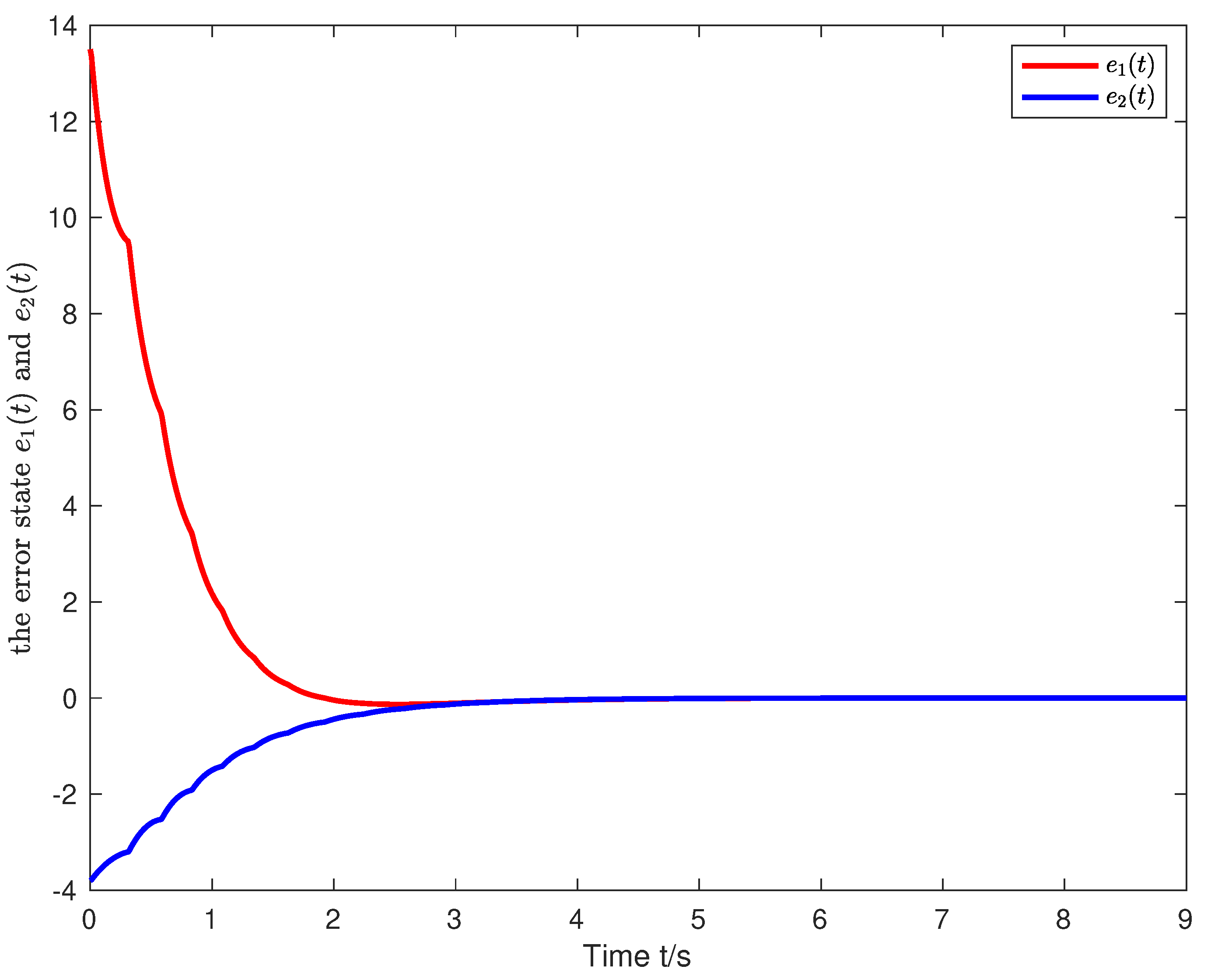
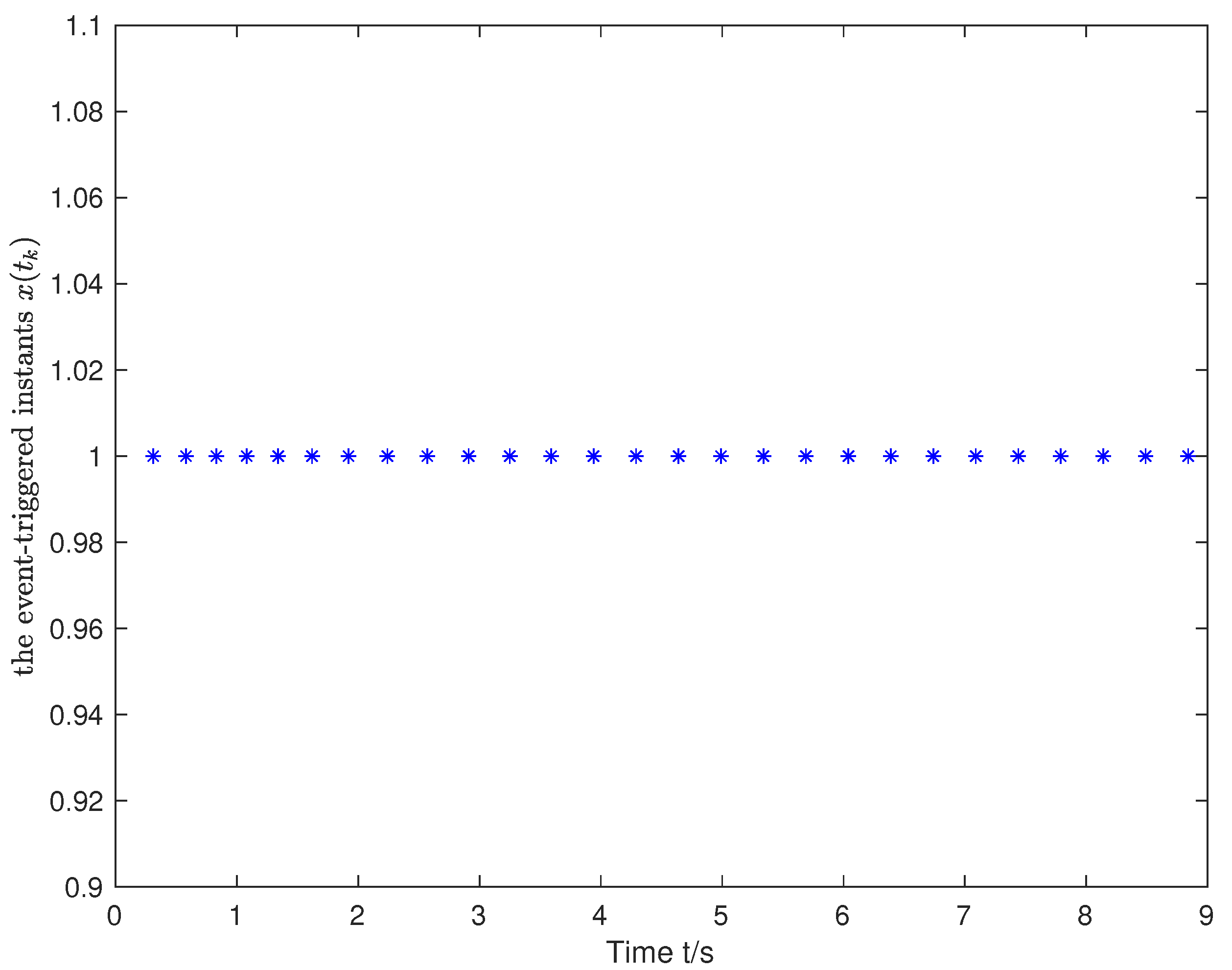
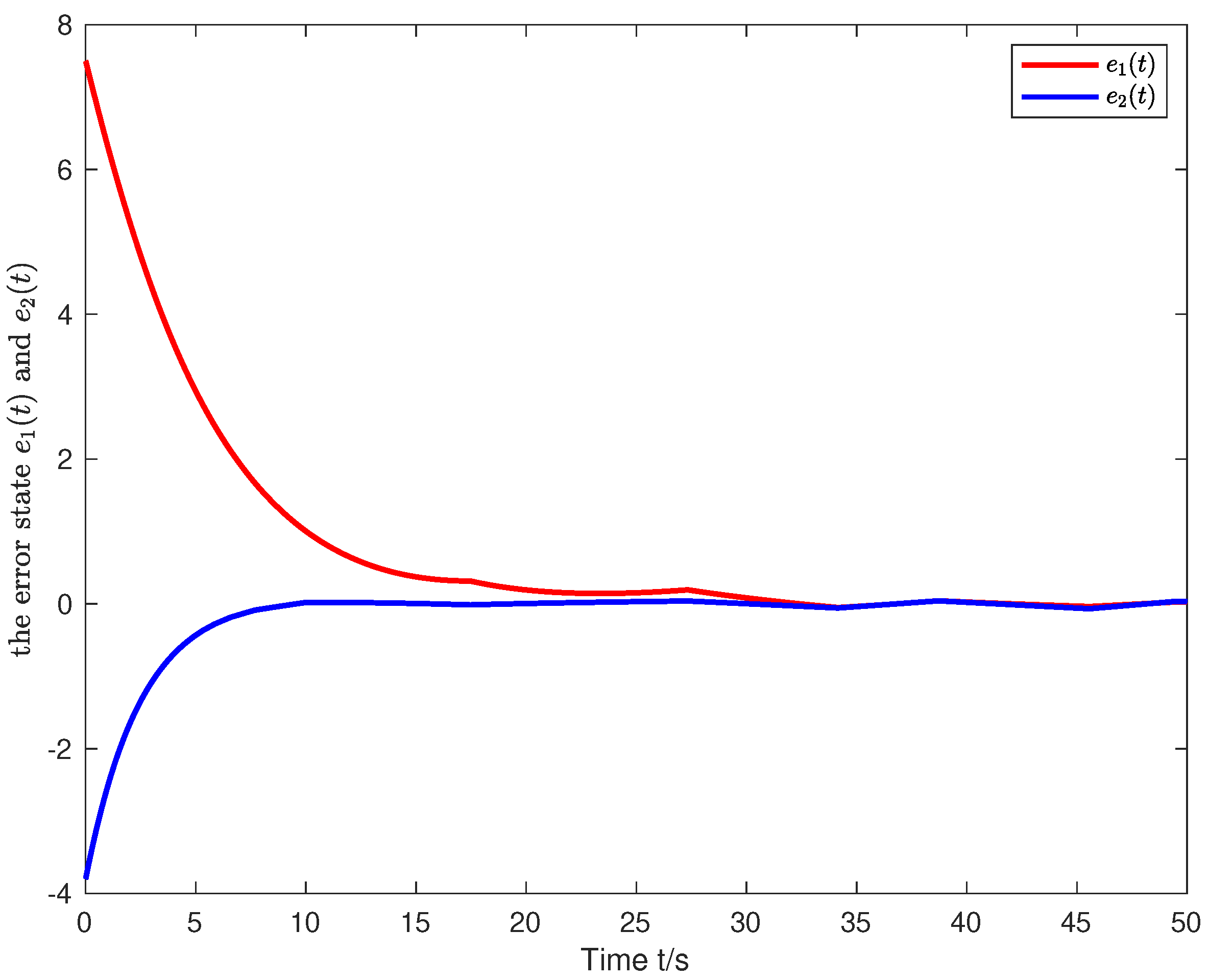
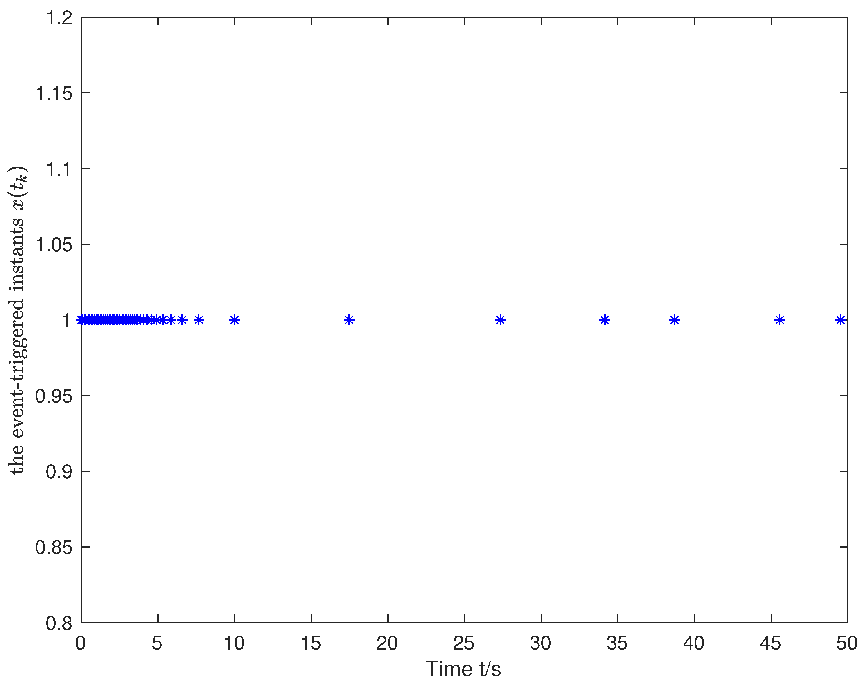
4. Numerical Examples and Simulations

In this section, two numerical examples and simulations are provided to illustrate the effectiveness of the theoretical results proposed in this paper.

Example 1.

Consider two-neurons FONNs as follows

$$\left\{\begin{array}{cc}\hfill D^{\alpha }x\left(t\right)& =Ax\left(t\right)+Bf\left(x\right(t\left)\right),\hfill \\ \hfill y\left(t\right)& =Cx\left(t\right),\hfill \end{array}\right.$$

where $x\left(t\right)={[x_1,x_2]}^T,y\left(t\right)={[y_1,y_2]}^T$. The parameter matrices are chosen to be

$$A=\left[\begin{array}{cc}-2& 0\\ 0& -1\end{array}\right],B=\left[\begin{array}{cc}-1& 2\\ 2& -3\end{array}\right],C=\left[\begin{array}{cc}3& 0\\ 0& 1\end{array}\right].$$

The activation functions for two neurons are selected to be $f\left(x\right)=[0.2cos\left(x_1\right),$$0.3cos\left(x_2\right){]}^T$. By choosing ${ϵ}_1={ϵ}_2=1$, it is concluded that there exist

$$L_1=\left[\begin{array}{cc}0.2& 0\\ 0& 0.1\end{array}\right],L_2=\left[\begin{array}{cc}-0.1& 0\\ 0& 0\end{array}\right],$$

such that assumption $\left({\mathrm{H}}_1\right)$ holds.

By taking $\alpha =0.96$ for the order of the Caputo fractional-order derivative and employing the MATLAB LMI toolbox, we obtain a set of feasible solutions for (29) to be $\gamma =0.418$ and

$$P=\left[\begin{array}{cc}0.5814& 0.0390\\ 0.0390& 0.3593\end{array}\right],Y=\left[\begin{array}{cc}0.0555& 0.0078\\ 0.0078& -0.1799\end{array}\right],R=\left[\begin{array}{cc}0.7782& 12.7137\\ 5.8530& -6.4755\end{array}\right].$$

Furthermore, on the basis of $K=P^{-1}Y$, we derive that the gain matrix of estimator

$$K=\left[\begin{array}{cc}0.0948& 0.0473\\ 0.0114& -0.5059\end{array}\right].$$

For the convenience of simulation, we take the initial values of the FONN and its estimator as $x\left(0\right)={[4.5,-3.8]}^T$ and $\widehat{x}\left(0\right)={[0,0]}^T$, respectively. With the help of MATLAB software, the simulation results for estimation error, the event-triggering instants, and the sampled output measurement are provided in Figure 1, Figure 2 and Figure 3. Specifically, Figure 1 shows that the estimation error system is globally Mittag–Leffler stable, which further indicates that the designed estimator can successfully track the real state information of the FONN. The instants of event triggering are presented in Figure 2 from which we see that the updating frequency of the output measurement is significantly reduced, while the desired estimation performance is maintained. Figure 3 depicts the sampled output measurement $y\left(t_k\right)$ and the real information of measurement output $y\left(t\right)$. It is observed that the sampled signals of the output measurement would not be updated until the next triggering instant.

Example 2.

Consider the tumor-immune system with fractional-order derivative, which is borrowed from [41]. The two-dimensional dynamical model is described as follows

$$D^{\alpha }x\left(t\right)=Ax\left(t\right)+f\left(x\left(t\right)\right),$$

where $\alpha =0.9$, $x\left(t\right)={[x_1\left(t\right),x_2\left(t\right)]}^T$. The nonlinear function

$$f\left(x\right)={[0.1184x_1\left(t\right)x_2\left(t\right)+0.1211,-0.00327x_2^2\left(t\right)-x_1\left(t\right)x_2\left(t\right)]}^T$$

and the parameter matrix is selected as

$$A=\left[\begin{array}{cc}-0.3746& 0\\ 0& 1.635\end{array}\right].$$

By choosing ${ϵ}_1={ϵ}_2=1$, it is concluded that there exist

$$L_1=\left[\begin{array}{cc}0.2& 0\\ 0& 0.1\end{array}\right],L_2=\left[\begin{array}{cc}-0.1& 0\\ 0& 0\end{array}\right],$$

such that $\left({\mathrm{H}}_1\right)$ holds.

By taking the parameter matrix for measurement output as

$$C=\left[\begin{array}{cc}3& 0\\ 0& -1\end{array}\right]$$

and using the MATLAB LMI toolbox to calculate a set of feasible solutions for (29), one gets $\gamma =0.08518$ for the threshold parameter of the event-triggered mechanism and

$$P=\left[\begin{array}{cc}0.2250& -0.0275\\ -0.0275& 0.0243\end{array}\right],Y=\left[\begin{array}{cc}0.0775& 0.0206\\ 0.0206& -0.1182\end{array}\right],R=\left[\begin{array}{cc}0.4482& 9.2276\\ 2.0183& 9.0474\end{array}\right].$$

It follows from $K=P^{-1}Y$ that

$$K=\left[\begin{array}{cc}0.5262& -0.5894\\ 1.4408& -5.5254\end{array}\right].$$

For the aim of simulations, we take the initial values of the fractional-order tumor-immune system and its estimator to be $x\left(0\right)={[2.5,3.8]}^T$ and $\widehat{x}\left(0\right)={[0,0]}^T$, respectively. By utilizing MATLAB software, the simulation results for the estimation error system and the event-triggering instants are presented in Figure 4 and Figure 5. In detail, Figure 4 shows that the estimation error system is globally Mittag–Leffler stable, which implies that the real state information of the fractional-order tumor-immune system can be estimated ultimately. Figure 5 illustrates that the instants of event triggering are dramatically reduced without loss of the final convergence property of the estimation error system.

5. Conclusions

In this paper, we considered the problem of event-triggered state estimation for a class of FONNs. For saving communication resources, an event-triggering strategy was adopted to reduce the frequency of data transmission between the output sensor and the estimator. Based on the Lyapunov method and properties of fractional-order calculus, the global Mittag-Leffler stability was investigated for estimation error system, and several sufficient criteria were proposed in the form of LMIs. Furthermore, the Zeno phenomenon in the event-triggering strategy was excluded via analyzing the evolution dynamics of measured error. The effectiveness of the proposed theoretical results was verified through two numerical examples and simulations. It is worth noting that the methodology used in this paper is also applicable to coupled networks and multi-agent systems with fractional-order derivative. In near future, we will focus on the event-triggered state estimation of fractional-order neural networks with time delay. Moreover, the dynamical event-triggered scheme will also be our next work.

References

1. Bao, H.; Park, J.H.; Cao, J. Synchronization of fractional-order complex-valued neural networks with time delay. Neural Netw. 2016, 81, 16–28. [Google Scholar] [CrossRef]
2. Velmurugan, G.; Rakkiyappan, R.; Vembarasan, V.; Cao, J.; Alsaedi, A. Dissipativity and stability analysis of fractional-order complex-valued neural networks with time delay. Neural Netw. 2017, 86, 42–53. [Google Scholar] [CrossRef]
3. Subramanian, K.; Muthukumar, P. Existence, uniqueness, and global asymptotic stability analysis for delayed complex-valued Cohen–Grossberg BAM neural networks. Neural Comput. Appl. 2018, 29, 565–584. [Google Scholar] [CrossRef]
4. Gunasekaran, N.; Zhai, G. Stability analysis for uncertain switched delayed complex-valued neural networks. Neurocomputing 2019, 367, 198–206. [Google Scholar] [CrossRef]
5. Tan, Y.; Liu, Y.; Niu, B.; Fei, S. Event-triggered synchronization control for T–S fuzzy neural networked systems with time delay. J. Frankl. Inst. 2020, 357, 5934–5953. [Google Scholar] [CrossRef]
6. Li, Y.; Xie, W.; Li, H. Hyperspectral image reconstruction by deep convolutional neural network for classification. Pattern Recognit. 2017, 63, 371–383. [Google Scholar] [CrossRef]
7. Zhang, S.; Yu, Y.; Yu, J. LMI conditions for global stability of fractional-order neural networks. IEEE Trans. Neural Netw. Learn. Syst. 2016, 28, 2423–2433. [Google Scholar] [CrossRef]
8. Cao, J.; Wang, J. Global asymptotic and robust stability of recurrent neural networks with time delays. IEEE Trans. Circuits Syst. Regul. Pap. 2005, 52, 417–426. [Google Scholar]
9. Yang, X.; Wan, X.; Zunshui, C.; Cao, J.; Liu, Y.; Rutkowski, L. Synchronization of switched discrete-time neural networks via quantized output control with actuator fault. IEEE Trans. Neural Netw. Learn. Syst. 2020, 32, 4191–4201. [Google Scholar] [CrossRef]
10. Tang, R.; Su, H.; Zou, Y.; Yang, X. Finite-Time Synchronization of Markovian Coupled Neural Networks With Delays via Intermittent Quantized Control: Linaear Programming Approach. IEEE Trans. Neural Netw. Learn. Syst. 2021. [Google Scholar] [CrossRef]
11. Zou, Y.; Su, H.; Tang, R.; Yang, X. Finite-time bipartite synchronization of switched competitive neural networks with time delay via quantized control. ISA Trans. 2021. [Google Scholar] [CrossRef]
12. Gao, Y.; Guo, X.; Yao, R.; Zhou, W.; Cattani, C. Stability analysis of neural network controller based on event triggering. J. Frankl. Inst. 2020, 357, 9960–9975. [Google Scholar] [CrossRef]
13. Yu, H.; Shang, J.; Chen, T. On stochastic and deterministic event-based state estimation. Automatica 2021, 123, 109314. [Google Scholar] [CrossRef]
14. Nagamani, G.; Shafiya, M.; Soundararajan, G.; Prakash, M. Robust State Estimation for Fractional-order Delayed BAM Neural Networks via LMI Approach. J. Frankl. Inst. 2020, 357, 4964–4982. [Google Scholar] [CrossRef]
15. Hu, B.; Song, Q.; Zhao, Z. Robust state estimation for fractional-order complex-valued delayed neural networks with interval parameter uncertainties: LMI approach. Appl. Math. Comput. 2020, 373, 125033. [Google Scholar] [CrossRef]
16. Diethelm, K. The Analysis of Fractional Differential Equations: An Application-Oriented Exposition Using Differential Operators of Caputo Type; Springer Science & Business Media: Berlin/Heidelberg, Germany, 2010. [Google Scholar]
17. Feng, T.; Wang, Y.E.; Liu, L.; Wu, B. Observer-based event-triggered control for uncertain fractional-order systems. J. Frankl. Inst. 2020, 357, 9423–9441. [Google Scholar] [CrossRef]
18. Kaslik, E.; Sivasundaram, S. Nonlinear dynamics and chaos in fractional-order neural networks. Neural Netw. 2012, 32, 245–256. [Google Scholar] [CrossRef]
19. Wang, H.; Song, Q. State estimation for neural networks with mixed interval time-varying delays. Neurocomputing 2010, 73, 1281–1288. [Google Scholar] [CrossRef]
20. Li, C.; Zhang, F. A survey on the stability of fractional differential equations. Eur. Phys. J. Spec. Top. 2011, 193, 27–47. [Google Scholar] [CrossRef]
21. Bao, H.; Cao, J.; Kurths, J. State estimation of fractional-order delayed memristive neural networks. Nonlinear Dyn. 2018, 94, 1215–1225. [Google Scholar] [CrossRef]
22. Wang, F.; Yang, Y.; Hu, M.; Xu, X. State estimation for fractional-order neural networks. Optik 2015, 126, 4083–4086. [Google Scholar] [CrossRef]
23. Liu, T.; Wei, Y.; Yin, W.; Wang, Y.; Liang, Q. State estimation for nonlinear discrete–time fractional systems: A Bayesian perspective. Signal Process. 2019, 165, 250–261. [Google Scholar] [CrossRef]
24. Gao, Z. Active disturbance rejection control for nonlinear fractional-order systems. Int. J. Robust Nonlinear Control. 2016, 26, 876–892. [Google Scholar] [CrossRef]
25. Li, B.; Wang, Z.; Ma, L.; Liu, H. Observer-based event-triggered control for nonlinear systems with mixed delays and disturbances: The input-to-state stability. IEEE Trans. Cybern. 2018, 49, 2806–2819. [Google Scholar] [CrossRef]
26. Wang, Y.; Ding, S.; Li, R. Master–slave synchronization of neural networks via event-triggered dynamic controller. Neurocomputing 2021, 419, 215–223. [Google Scholar] [CrossRef]
27. Xing, X.; Liu, J. Event-triggered neural network control for a class of uncertain nonlinear systems with input quantization. Neurocomputing 2021, 440, 240–250. [Google Scholar] [CrossRef]
28. Yang, H.; Wang, Z.; Shen, Y.; Alsaadi, F.E.; Alsaadi, F.E. Event-triggered state estimation for Markovian jumping neural networks: On mode-dependent delays and uncertain transition probabilities. Neurocomputing 2021, 424, 226–235. [Google Scholar] [CrossRef]
29. Heemels, W.P.; Johansson, K.H.; Tabuada, P. An introduction to event-triggered and self-triggered control. In Proceedings of the 2012 IEEE 51st IEEE Conference on Decision and Control (CDC), Maui, HI, USA, 10–13 December 2012; pp. 3270–3285. [Google Scholar]
30. Ge, X.; Han, Q.L.; Zhang, X.M.; Ding, L.; Yang, F. Distributed event-triggered estimation over sensor networks: A survey. IEEE Trans. Cybern. 2019, 50, 1306–1320. [Google Scholar] [CrossRef]
31. Qin, J.; Ma, Q.; Shi, Y.; Wang, L. Recent advances in consensus of multi-agent systems: A brief survey. IEEE Trans. Ind. Electron. 2016, 64, 4972–4983. [Google Scholar] [CrossRef]
32. Liu, Y.; Tang, R.; Zhou, C.; Xiang, Z.; Yang, X. Event-triggered leader-following consensus of multiple mechanical systems with switched dynamics. Int. J. Syst. Sci. 2020, 51, 3563–3572. [Google Scholar] [CrossRef]
33. Yu, N.; Zhu, W. Event-triggered impulsive chaotic synchronization of fractional-order differential systems. Appl. Math. Comput. 2021, 388, 125554. [Google Scholar] [CrossRef]
34. Shi, M.; Hu, S.; Yu, Y. Generalised exponential consensus of the fractional-order nonlinear multi-agent systems via event-triggered control. Int. J. Syst. Sci. 2019, 50, 1244–1251. [Google Scholar] [CrossRef]
35. Podlubny, I. Fractional Differential Equations; Academic Press: San Diego, CA, USA, 1999. [Google Scholar]
36. Duarte-Mermoud, M.A.; Aguila-Camacho, N.; Gallegos, J.A.; Castro-Linares, R. Using general quadratic Lyapunov functions to prove Lyapunov uniform stability for fractional order systemsa. Commun. Nonlinear Sci. Numer. Simul. 2015, 22, 650–659. [Google Scholar] [CrossRef]
37. Song, Q.; Chen, Y.; Zhao, Z.; Liu, Y.; Alsaadi, F.E. Robust stability of fractional-order quaternion-valued neural networks with neutral delays and parameter uncertainties. Neurocomputing 2021, 420, 70–81. [Google Scholar] [CrossRef]
38. Boyd, S.; El Ghaoui, L.; Feron, E.; Balakrishnan, V. Linear Matrix Inequalities in System and Control Theory; SIAM: Philadelphia, PA, USA, 1994. [Google Scholar]
39. Zhang, S.; Yu, Y.; Wang, H. Mittag-Leffler stability of fractional-order Hopfield neural networks. Nonlinear Anal. Hybrid Syst. 2015, 16, 104–121. [Google Scholar] [CrossRef]
40. Li, Y.; Chen, Y.; Podlubny, I. Stability of fractional-order nonlinear dynamic systems: Lyapunov direct method and generalized Mittag–Leffler stability. Comput. Math. Appl. 2010, 59, 1810–1821. [Google Scholar] [CrossRef] [Green Version]
41. Rihan, F.; Hashish, A.; Al-Maskari, F.; Hussein, M.; Ahmed, E.; Riaz, M.; Yafia, R. Dynamics of tumor-immune system with fractional-order. J. Tumor Res. 2016, 2, 109–115. [Google Scholar] [CrossRef]
Figure 1. The evolution of estimation error state e ( t ) .
Mathematics 10 00325 g001
Figure 2. The sequence of event-triggered instants t k .
Mathematics 10 00325 g002
Figure 3. The sampled output measurement y ( t k ) and the measurement output y ( t ) .
Mathematics 10 00325 g003
Figure 4. The evolution of estimation error state e ( t ) .
Mathematics 10 00325 g004
Figure 5. The sequence of event-triggered instants t k .
Mathematics 10 00325 g005
Publisher’s Note: MDPI stays neutral with regard to jurisdictional claims in published maps and institutional affiliations.