Article

Turing Instability and Spatiotemporal Pattern Formation Induced by Nonlinear Reaction Cross-Diffusion in a Predator–Prey System with Allee Effect

School of Mathematics and Physics, University of Science and Technology Beijing, Beijing 100083, China
*
Author to whom correspondence should be addressed.
Mathematics 2022, 10(9), 1500; https://doi.org/10.3390/math10091500
Submission received: 11 March 2022 / Revised: 23 April 2022 / Accepted: 25 April 2022 / Published: 1 May 2022

Abstract

:
The Allee effect is widespread among endangered plants and animals in ecosystems, suggesting that a minimum population density or size is necessary for population survival. This paper investigates the stability and pattern formation of a predator–prey model with nonlinear reactive cross-diffusion under Neumann boundary conditions, which introduces the Allee effect. Firstly, the ODE system is asymptotically stable for its positive equilibrium solution. In a reaction system with self-diffusion, the Allee effect can destabilize the system. Then, in a reaction system with cross-diffusion, through a linear stability analysis, the cross-diffusion coefficient is used as a bifurcation parameter, and instability conditions driven by the cross-diffusion are obtained. Furthermore, we show that the system (5) has at least one inhomogeneous stationary solution. Finally, our theoretical results are illustrated with numerical simulations.

1. Introduction

Starting with the seminal research of Lotka and Volterra, the analysis of predator–prey model has become an important field of mathematical biology because of its practical and theoretical significance. Most articles about the simulation of predator–prey interaction use the logistic growth function. Meanwhile, some examples verify the existence of the Allee effect, which Allee proposed [1]. The Allee effect has many possible origins, e.g., difficulty looking for a partner, reproductive convenience, environmental regulation, or close relative decline. In general, for a population that is initially low density, if the per capita growth rate is an increasing function, then the species has an Allee effect. The Allee effect is divided into strong and weak; if the growth rate per capita is negative in a low-density limit, this is a strong Allee effect, while a weak Allee effect is expressed at zero density when the per capita growth rate is positive. A strong Allee effect creates a population threshold beyond which the population could grow. On the contrary, a group with a weak Allee effect has no threshold [2,3,4]. Prey is influenced by strong Allee effects. Numerous studies have revealed rich and diverse pattern-formation scenarios. Especially in a predator–prey system with a strong Allee effect on the population of the prey, space is vital for existence of species. Pattern formation can be observed both inside and outside the Turing field. Especially in reaction-diffusion systems, the function of space is significant for the existence of a species. On the other hand, numerous studies have shown that pattern formation is altered with the addition of a weak Allee effect. Currently, the Allee effect receives great attention from ecologist and mathematicians, because it can affect the population growth of a species [5,6,7,8,9,10,11,12].
In 1952, Turing proposed that space-diffusion can destroy interacting chemicals in a homogeneous and stable state, which is occurs through two coupled reaction–diffusion equations. This instability is known as diffusion-driven instability or Turing instability [13,14]. In recent years, reaction–diffusion systems have attracted increasing attention from mathematical biologists seeking insights into patterns occurring in ecosystems [15,16,17,18,19,20,21,22,23,24,25,26]. Many researchers have studied the emergence of patterns in population dynamics systems with self-diffusion [27,28,29,30,31]. While the reaction–diffusion system is not sterically stable, it exhibits Turing modes in space. With the broad growth of biomathematics and theoretical biology, the most prominent theme in the scopes of the dynamic system is the influence of cross-diffusion on mode appearance [32,33,34,35,36,37,38]. Biologically, integrated defenses against prey tend to move predators to areas with lower prey concentrations, which means that this can give rise to a spatially inhomogeneous population distribution. This can be described by reaction–diffusion systems with cross-diffusion. It has been seen that a appropriate cross-diffusion coefficient is able to generate this pattern [39,40,41].
In view of the above introduction about the Allee effect and the diffusion term, some scholars have studied the impact of the Allee effect on the stability and the pattern formation of the predator–prey system, and some scholars have studied the impact of diffusion on the stability and the pattern formation of the system. By studying the temporal and spatial distribution and dynamics of populations, human beings can better protect and adjust populations and rationally develop and utilize resources, which has far-reaching significance. Due to the aforementioned motivations, in this paper, we consider the effects of the Allee effect and nonlinear cross-diffusion terms on system stability and spatial mode formation in our model. The structure of the text is as follows: in Section 2, in terms of its mathematical and biological significance, we introduce the model. In Section 3, we discuss the influence of the Allee effect constant on the stability of the coexistence equilibrium of the predator–prey system with self-diffusion and ODE systems. Additionally, the conditions of cross-diffusion-driven Turing instability are obtained. In Section 4, we prove the existence of a nonconstant positive solution. In Section 5, our theoretical results are illustrated with numerical simulations. Finally, in Section 6, the conclusion is given.

2. The Mathematical Model

In the section, firstly, we introduce the Allee effect into the prey growth function.
In 1983, Verhulst–Pearl proposed the Verhulst–Pearl equation, which is also called the Logistic model:
d U d t = r m U ( 1 U K ) ,
U ( t ) is species density, K is carrying capacity, also known as environmental capacity, and it is a constant. r m is defined as the intrinsic growth rate. At this time, the average growth rate is r = r m ( 1 U K ) . When the population density reaches K , the birth rate is equal to the death rate.
The following model is used to describe the growth of a single population:
d U d t 1 U = e ( 1 U P ) g ,
e is the birth rate per capita when undisturbed by other individuals; when the actual birth rate per capita is zero, the density of the population is P . g is the per capita mortality rate for adults. Equation (2) is equivalent to the logistic equation, and environmental carrying capacity is K = P ( e g ) / e [42]. Introducing the Allee effect to Equation (2):
d U d t 1 U = e ( 1 U P ) ( U U + m ) g ,
m is the Allee effect constant, and U / U + m is known as the Allee effect, where the larger the m , the better the Allee effect. Solving equation e ( 1 U P ) ( U U + m ) g = 0 , the equivalent equation is e U 2 P ( e g ) U + P g m = 0 . Assuming Δ 0 = [ P ( e g ) ] 2 4 P e g m > 0 , let l = P ( e g ) Δ 0 2 e ,   k = P ( e g ) + Δ 0 2 e . Additionally, Equation (3) can also be expressed as:
d U d t 1 U = e ( 1 U P ) ( U U + m ) g = e ( U l ) ( k U ) P ( U + m ) ,
Equation (4) can be simplified to: d u d t = ω u ( 1 u ) ( u β ) σ + u , where u = U K , ω = K e P , β = l K , σ = m K .
Let u 1 ,   u 2 denote the density of prey and predator. Let y = ( u 1 ,   u 2 ) T , D ( y ) = ( D i j ( y ) ) 2 × 2 . y t = Δ [ D ( y ) ] + H ( y ) represents the strongly coupled reaction–diffusion system. Concerning the nonlinear cross-diffusion coefficient, the authors of [43,44] researched the systems for D ( y ) = d i g ( c 1 + k ε + u 3 2 , c 2 , c 3 ) y , D ( y ) = d i g ( c 1 + k ε + u 3 2 , c 2 , c 3 + c 3 c 4 u 1 ) y . Additionally, here, we study the system for D ( y ) = d i g ( c 1 + k η + u 2 2 , c 2 + c 4 u 1 ) y . It can be simplified to D ( y ) = d i g ( c 1 + c 3 1 + c 5 u 2 2 , c 2 + c 4 u 1 ) y , where c 3 = k η , c 5 = 1 η .
In this article, we study a predator–prey model with the Allee effect and nonlinear cross-diffusion.
{ u 1 t Δ ( c 1 + c 3 1 + c 5 u 2 2 ) u 1 = ω u 1 ( 1 u 1 ) ( u 1 β ) σ + u 1 u 1 u 2 ,   t > 0 ,   x Ω , u 2 t c 2 Δ ( 1 + c 4 u 1 ) u 2 = u 1 u 2 δ u 2 ,   t > 0 ,   x Ω , u 1 n = u 2 n = 0 ,     t > 0 ,   x Ω , u i ( x , 0 ) = u i 0 ( x ) 0 , i = 1 , 2 ,   x Ω ,
u 1 ( x ) and u 2 ( x ) are the population densities of prey and predator, respectively. ω is the intrinsic prey growth rate, and δ represents the relative mortality of the predator. σ is the Allee effect constant and β is the Allee threshold. c 1 , c 2 , c 3 , c 4 and c 5 are positive constants, the constants c m ( m = 1 ,   2 ) are termed self-diffusion coefficients, and c m ( m = 3 ,   4 ) are termed cross-diffusion coefficients. Ω is a bounded domain in R N with a smooth boundary Ω . The Homogeneous Neumann boundary condition states the population flux across the boundary is zero.
The diffusive flux of u 1 is
J = ( c 1 u 1 + c 3 u 1 1 + c 5 u 2 2 ) = ( c 1 + c 3 1 + c 5 u 2 2 ) u 1 + 2 c 3 c 5 u 1 u 2 ( 1 + c 5 u 2 2 ) 2 u 2 ,
as 2 c 3 u 1 u 2 / ( 1 + c 5 u 2 2 ) 2 0 , the 2 c 3 u 1 u 2 / ( 1 + c 5 u 2 2 ) 2 u 2 part of the flux is in the direction of the increasing population density of u 2 .
The diffusive flux of u 2 is
J = ( c 2 u 2 + c 2 c 4 u 1 u 2 ) = c 2 c 4 u 2 u 1 ( c 2 + c 2 c 4 u 1 ) u 2 ,
as c 2 c 4 u 2 < 0 , c 2 c 4 u 2 u 1 of the flux is in the direction of the decreasing population density of   u 1 .
As predators hunt their prey, the flux should point in the direction of increasing prey population density. However, in certain ecosystems, large numbers of prey species come together to form a large group to protect themselves from predators.

3. Stability of the Coexisting Equilibrium

In this section, we discuss the effect of the Allee effect constant on the stability of the coexistence equilibrium point of ODE systems and predator–prey systems with self-diffusion. When ( 1 δ ) ( δ β ) > 0 , y ˜ = ( u ˜ 1 ,   u ˜ 2 ) is the unique positive coexistence equilibrium point in system (5), where
u ˜ 1 = δ , u ˜ 2 = ω ( 1 δ ) ( δ β ) σ + δ .
Consider the ODE system of system (5) as follows:
{ d u 1 d t = ω u 1 ( 1 u 1 ) ( u 1 β ) σ + u 1 u 1 u 2 ,   t > 0 , d u 2 d t = u 1 u 2 δ u 2 ,                     t > 0 .  
Theorem 1.
If the parameters of (5) satisfy
σ > β δ 2 2 δ β 1
u ˜ is locally asymptotically stable in system (7).
Proof. 
Indicate
H ( y ) = ( H 1 ( y ) H 2 ( y ) ) = ( u 1 g 1 ( y ) u 1 ( ω ( 1 u 1 ) ( u 1 β ) σ + u 1 u 2 ) u 2 g 2 ( y ) u 2 ( u 1 δ ) ) = ( u 1 ( ω ( u 1 2 + ( β + 1 ) u 1 β ) σ + u 1 u 2 ) u 2 ( u 1 δ ) ) .
Noticing H ( y ˜ ) = 0 ,
H u ( y ˜ ) = ( u ˜ 1 ( ω u ˜ 1 2 2 ω σ u ˜ 1 + ω σ β + ω σ + ω β ( σ + u ˜ 1 ) 2 ) u ˜ 1 u ˜ 2 0 ) .
The characteristic polynomial of H y ( y ˜ ) is
χ ( η ) = η 2 + A 1 η + A 2 ,
where A 1 = T r a c e ( H y ( y ˜ ) ) ,   A 2 = D e t ( H y ( y ˜ ) ) .
If (8) holds, A 1 and A 2 are positive, which is easy to verify. So, due to the Routh–Hurwitz criterion, a conclusion is established. □
Next, the following system (5) with self-diffusion can be studied:
{ u 1 t c 1 Δ u 1 = ω u 1 ( 1 u 1 ) ( u 1 β ) σ + u 1 u 1 u 2 ,   t > 0 ,   x Ω , u 2 t c 2 Δ u 2 = u 1 u 2 δ u 2 , t > 0 ,   x Ω , u 1 n = u 2 n = 0 ,     t > 0 ,   x Ω , u i ( x , 0 ) = u i 0 ( x ) 0 , i = 1 , 2 ,   x Ω .
To research the local asymptotic stability of Equation (11), similar to [45], we give Notation 1.
Notation 1.
Let 0 = π 1 < π 2 < be the eigenvalues of Δ on Ω under no-flux boundary conditions, and let E ( π m ) be the space of eigenfunctions corresponding to π m . Then,
(i)
X m n : = { c ϕ m n : c R 3 } , { ϕ m n } are the orthonormal bases of E ( π m ) , n = 1 , 2 dim E ( π m ) .
(ii)
X : = { u [ C 1 ( Ω ¯ ) ] 3 : n u 1 = n u 2 = 0   o n   Ω } , then X = m = 1 X m , X m = n = 1 dim E ( π m ) X m n .
Theorem 2.
If (8) holds, y ˜ is locally asymptotically stable in system (11).
Proof. 
Linearizing system (11), then
y t = ( D Δ + H y ( y ˜ ) ) y
where D = ( c 1 0 0 c 2 ) .
Due to Notation 1, if and only if X m is an eigenvalue of the matrix π m D + H y ( y ˜ ) , it is invariant under operator D Δ + H y ( y ˜ ) , when this operator on X m , λ is an eigenvalue. ψ m ( λ ) = | λ E ( π m D + H y ( π ) ) | = λ 2 + B 1 λ + B 2 is the characteristic polynomial of π m D + H y ( y ˜ ) , where
B 1 = π m c 1 + π m c 2 + u ˜ 1 ( ω u ˜ 1 2 + 2 ω σ u ˜ 1 ( ω β σ + ω σ + ω β ) ( σ + u ˜ 1 ) 2 ) ,
B 2 = u ˜ 1 u ˜ 2 + π m c 2 ( π m c 1 + u ˜ 1 ( ω u ˜ 1 2 + 2 ω σ u ˜ 1 ( ω β σ + ω σ + ω β ) ( σ + u ˜ 1 ) 2 ) ) .  
If (8) holds, we are able to show that B 1 and B 2 are positive. Then, for each i 1 , because of the Routh–Hurwitz criterion, the two roots λ i 1 ,   λ i 2 0 of ψ i ( λ ) = 0 have negative real parts. So, the conclusion holds. □
Theorem 3.
Assume that
2 c 5 u ˜ 2 ( c 2 + c 2 c 4 u ˜ 1 ) ( 1 + c 5 u ˜ 2 2 ) + 2 c 5 c 2 c 4 u ˜ 2 > 0
and (8) hold, if π 2 < μ ˜ , where π 2 can be seen in Notation 1, μ ˜ will be seen in (14). There must be a positive constant c 3 , when the c 3 c 3 , coexistence equilibrium solution y ˜ of system (5) is unstable.
Proof. 
We indicate that
ϑ ( y ) = ( c 1 u 1 + c 3 u 1 1 + c 5 u 2 2 , c 2 u 2 + c 2 c 4 u 1 u 2 ) T
Linearizing system (5) at y ˜ , then we have y t = ( ϑ y Δ + H y ( y ˜ ) ) y , where
ϑ y = ( c 1 + c 3 1 + c 5 u ˜ 2 2 2 c 3 c 5 u ˜ 1 u ˜ 2 2 ( 1 + c 5 u ˜ 2 2 ) 2 c 2 c 4 u ˜ 2 c 2 + c 2 c 4 u ˜ 1 ) ,
the characteristic polynomial of π m ϑ y + H y ( y ˜ ) is ς m ( λ ) = λ 2 + B ¯ 1 λ + B ¯ 2 ,
B ¯ 1 = π m ( c 1 +   c 3 1 + c 5 u ˜ 2 2 + c 2 + c 2 c 4 u ˜ 1 ) u ˜ 1 ( ω u ˜ 1 2 2 ω σ u ˜ 1 + ω σ β + ω σ + ω β ( σ + u ˜ 1 ) 2 ) , B ¯ 2 = π m 2 ( ( c 1 + c 3 1 + c 5 u ˜ 2 2 ) ( c 2 + c 2 c 4 u ˜ 1 ) + 2 c 5 c 2 c 3 c 4 u ˜ 2 ( 1 + c 5 u ˜ 2 2 ) ) + π m ( u ˜ 1 ( ω u ˜ 1 2 2 ω σ u ˜ 1 + ω σ β + ω σ + ω β ( σ + u ˜ 1 ) 2 ) ( c 2 + c 2 c 4 u ˜ 1 ) c 2 c 4 u ˜ 1 u ˜ 2 2 c 3 c 5 u ˜ 2 ( 1 + c 5 u ˜ 2 2 ) ) + u ˜ 1 u ˜ 2 .
Let λ 1 ( π m ) , λ 2 ( π m ) be the two roots of ς m ( λ ) = 0 , and λ 1 ( π m ) λ 2 ( π m ) = B ¯ 2 . To have at least one Re ( λ m ) > 0 , B ¯ 2 < 0 is enough. Next, we find the condition for B ¯ 2 < 0 . B ¯ 2 = det ( π m Φ y H y ( y ˜ ) ) and B ¯ 2 = Q 2 π m 2 + Q 1 π m + Q 0 , where
Q 2 = ( c 1 + c 3 1 + c 5 u ˜ 2 2 ) ( c 2 + c 2 c 4 u ˜ 1 ) + 2 c 5 c 2 c 3 c 4 u ˜ 2 ( 1 + c 5 u ˜ 2 2 ) ,
Q 1 = u ˜ 1 ( ω u ˜ 1 2 2 ω σ u ˜ 1 + ω σ β + ω σ + ω β ( σ + u ˜ 1 ) 2 ) ( c 2 + c 2 c 4 u ˜ 1 ) c 2 c 4 u ˜ 1 u ˜ 2 2 c 3 c 5 u ˜ 2 ( 1 + c 5 u ˜ 2 2 ) ,  
Q 0 = u ˜ 1 u ˜ 2 , det ( H y ) = u ˜ 1 u ˜ 2 .  
Let Q ˜ ( π ) = Q 2 π 2 + Q 1 π + det ( H y ) and π ˜ 1 , π ˜ 2 , two roots of Q ˜ ( π ) = 0 , satisfy Re ( π ˜ 1 ) Re ( π ˜ 2 ) . Then, det ( H y ) = π ˜ 1 π ˜ 2 > 0 .
lim c 3 Q 2 c 3 = ( 1 1 + c 5 u ˜ 2 2 ) ( c 2 + c 2 c 4 u ˜ 1 ) + 2 c 5 c 2 c 4 u ˜ 2 ( 1 + c 5 u ˜ 2 2 ) , lim c 3 Q 1 c 3 = 2 c 5 u ˜ 2 ( 1 + c 5 u ˜ 2 2 ) .  
Note that
lim c 3 Q ˜ ( π ) c 3 = lim c 3 Q 2 π 2 + Q 1 π + det ( H u ) c 3 = ( ( 1 1 + c 5 u 2 2 ) ( c 2 + c 2 c 4 u ˜ 1 ) + 2 c 5 c 2 c 4 u ˜ 2 ( 1 + c 5 u ˜ 2 2 ) ) π m 2 + ( 2 c 5 u ˜ 2 ( 1 + c 5 u ˜ 2 2 ) ) π m .
Under condition (13), coherence contention is demonstrated; when c 3 is big enough, Re ( π ˜ 1 ) > 0 . Moreover, as Re ( π ˜ 1 ) Re ( π ˜ 2 ) > 0 , Re ( π ˜ 2 ) > 0 , and
lim c 3 π ˜ 1 = 2 c 5 u ˜ 2 ( c 2 + c 2 c 4 u ˜ 1 ) ( 1 + c 5 u ˜ 2 2 ) + 2 c 5 c 2 c 4 u ˜ 2 μ ˜ lim c 3 π ˜ 2 = 0 ,
So, there must be a constant c 3 , when c 3 > c 3 , the following holds: Q ˜ ( π ) < 0 ,   π ( π ˜ 2 , π ˜ 1 ) . Since that 0 < π 2 < π ˜ , that is
2 c 5 u ˜ 2 ( d 2 + d 2 d 4 u ˜ 1 ) ( 1 + c 5 u ˜ 2 2 ) + 2 c 5 d 2 d 4 u ˜ 2 > 0 .
We have π 2 ( π ˜ 2 , π ˜ 1 ) , so it follows that Q ˜ ( π 2 ) < 0 . Thus, we show that B ¯ 2 < 0 , and the proof is completed. □
It can be seen from the above theorem that cross-diffusion makes the positive equilibrium solution unstable.

4. Nonhomogeneous Steady States

In this section, our research concerns inhomogeneous positive solutions from the Leray–Schauder theory [45].
Firstly, we study the following form of the corresponding steady state of system (5):
{ Δ ( c 1 u 1 + c 3 u 1 1 + c 5 u 2 2 ) = ω u 1 ( 1 u 1 ) ( 1 β ) σ + u 1 u 1 u 2 ,   x Ω , c 2 Δ ( u 2 + c 4 u 1 u 2 ) = u 1 u 2 δ u 2 ,   x Ω .
Domain Ω determines the generic constants S ,   S _ ,   S _ . A collection is defined: B ( S ) = { y = ( u 1 , u 2 ) T : S _ < u i < S _ , i = 1 , 2 } , then in the set B ( S ) , we can obtain nonhomogeneous positive solutions.
Let ϑ ( y ) = ( c 1 u 1 + c 3 u 1 1 + c 5 u 2 2 , c 2 u 2 + c 4 u 1 u 2 ) T . Next, (15) is equivalent to
{ Δ ϑ ( y ) = H ( y ) ,   t > 0 ,   x Ω , n y = 0 ,   x Ω .
For y , ϑ y ( y ) exists and ϑ y ( y ) > 0 , the determinant of ϑ y ( y ) > 0 . So, y > 0 to (22) when
R ( y ) : = ( I Δ ) 1 { ϑ y 1 [ H ( y ) + y Φ y y ( y ) y ] + y } = y ,
( I Δ ) 1 is the inverse of I Δ under no-flux boundary constraints. Observe
R y ( y ˜ ) = ( I Δ ) 1 { Φ y 1 ( y ˜ ) H y ( y ˜ ) + I } ,
For the problem of eigenvalue
{ ( I R y ( y ˜ ) ) Ψ = λ Ψ ,   x Ω , n Ψ = 0 ,   x Ω ,
Ψ = ( Ψ 1 , Ψ 2 , Ψ 3 ) T . Since R ( ) has no fixed points in B ( S ) , the Leray–Schauder degree is well defined. Utilizing the Leray–Schauder theorem,
i n d e x ( I R ( ) , y ˜ ) = ( 1 ) τ ,   τ = Σ ξ > 0 n ξ ,
If zero is not the eigenvalue of (17), n ξ is the multiplicity of ξ .
If and only if ξ is an eigenvalue of the matrix I + 1 1 + π m ( ϑ y 1 y ˜ H y ( y ˜ ) + I ) = 1 1 + π m ( π m I + ϑ y 1 ( y ˜ ) H y ( y ˜ ) ) ,   m   1 , 1 n dim   E ( π m ) , X m n is invariant under I + D y f ( y * ) . The number of positive eigenvalues ξ in X m n is odd if and only if det ( π m I + ϑ y 1 ( y ˜ ) H y ( y ˜ ) ) > 0 . Set
L ( π ) = L ( y ˜ , π ) det ( π I + ϑ y 1 ( y ˜ ) H y ( y ˜ ) ) ,
and next, we obtain some consequences.
Proposition 1.
Assume that all m 1 , matrix π m I + π y 1 ( y ˜ ) H y ( y ˜ ) is nonsingular. So, i n d e x ( I R ( ) , y ˜ ) = ( 1 ) τ ,     τ = Σ m 1 , H ( π m ) > 0 dim E ( π m ) .
For our convenience to compute i n d e x ( I R ( ) , y ˜ ) , next, we study the sign of L ( π m ) , fix c 1 , c 2 , c 4 , and consider the dependence of L ( π m ) on c 3 . Then, we note
L ( π ) = det { ϑ y 1 ( y ˜ ) ) det ( π ϑ y y ˜ H y ( y ˜ ) } .  
Now that we have determined det { π ϑ y ( y ˜ ) } > 0 , we just need to study det { π Φ y y ˜ H y ( y ˜ ) } . Actually, the value of obtained fromSection 3is equal to det { π ϑ y y ˜ H y ( y ˜ ) } . We obtain enough conditions to B ¯ 2 < 0 during the proof of Theorem 3.
Proposition 2.
Suppose (3.8) holds. There must be a constant c 3 * , for all c 3 c 3 * , two roots π ˜ 1 , π ˜ 2 of det { π ϑ y ( y ˜ ) H y ( y ˜ ) } = 0 are real and satisfy (3.9). Furthermore,
{ 0 < π ˜ 1 < π ˜ 2 , det { π ϑ y y ˜ H y ( y ˜ ) } > 0 ,   π ( , π ˜ 2 ) ( π ˜ 1 , ) , det { π ϑ y y ˜ H y ( y ˜ ) } < 0 ,   π ( π ˜ 2 , π ˜ 1 ) .
We study the influence of cross-diffusion on the positive solution of (16); firstly, we conclude that there is no nonconstant equilibrium solution without cross-diffusion.
Theorem 4.
Assume that
c 2 δ π 2 , c 3 = 0 , c 4 = 0 ,
which π 2 can see in Notation 1. Next, there must be a positive constant D ¯ 1 ; when c 1 D ¯ 1 , (15) has no nonconstant positive solution; moreover,
u i u ¯ i ,   i = 1 , 2   where   u ¯ i 1 | Ω | Ω u i d x .
Proof. 
Let u ¯ i 1 | Ω | Ω u i d x , i = 1 , 2 . Multiplying the ith equation of (15) through u i u ¯ i , then integrating the results over Ω by parts yields
c 1 Ω | u 1 | 2 = Ω ( u 1 u ¯ 1 ) ( u 1 g 1 ( u 1 , u 2 ) u ¯ 1 g 1 ( u ¯ 1 , u ¯ 2 ) ) d x = Ω ( u 1 u ¯ 1 ) ( u 1 ( ω ( 1 u 1 ) ( u 1 β ) σ + u 1 u 2 ) u ¯ 1 ( ω ( 1 u ¯ 1 ) ( u ¯ 1 β ) σ + u ¯ 1 u ¯ 2 ) ) d x = Ω ( u 1 u ¯ 1 ) 2 [ ( ω σ + ω σ β ) ( u 1 + u ¯ 1 ) + ( ω β ω + ω ( u 1 + u ¯ 1 ) u 1 u ¯ 1 ) ω σ β ω σ ( u ¯ 1 2 + u ¯ 1 u 1 + u 1 2 ) ( σ + u 1 ) ( σ + u ¯ 1 ) ] d x + Ω ( u 1 u ¯ 1 ) ( u ¯ 1 u ¯ 2 u 1 u 2 ) d x ,
c 2 Ω | u 2 | 2 = Ω ( u 2 u ¯ 2 ) ( u 2 g 2 ( u 1 , u 2 ) u ¯ 2 g 2 ( u ¯ 1 , u ¯ 2 ) ) d x = Ω ( u 2 u ¯ 2 ) ( u 2 ( u 1 δ ) u ¯ 2 ( u ¯ 1 δ ) ) d x = Ω ( u 1 u ¯ 1 ) 2 ( δ ) d x + Ω ( u 2 u ¯ 2 ) ( u 2 u 1 u ¯ 2 u ¯ 1 ) d x .  
  c 1 Ω | u 1 | 2 + c 2 Ω | u 2 | 2 = Ω ( u 1 u ¯ 1 ) 2 [ ( ω σ + ω σ β ) ( u 1 + u ¯ 1 ) + ( ω β ω + ω ( u 1 + u ¯ 1 ) u 1 u ¯ 1 ) ω σ β ω σ ( u ¯ 1 2 + u ¯ 1 u 1 + u 1 2 ) ( σ + u 1 ) ( σ + u ¯ 1 ) ] d x + Ω ( u 1 u ¯ 1 ) 2 ( δ ) d x + Ω ( u 1 u ¯ 1 ) ( u 2 u ¯ 2 ) ( u ¯ 1 u ¯ 2 u 1 u 2 u 2 u ¯ 2 + u 1 u 2 u ¯ 1 u ¯ 2 u 1 u ¯ 1 ) d x .
By the Cauchy inequality,
  c 1 Ω | u 1 | 2 + c 2 Ω | u 2 | 2 Ω ( u 1 u ¯ 1 ) 2 [ ( ω σ + ω σ β ) ( u 1 + u ¯ 1 ) + ( ω β ω + ω ( u 1 + u ¯ 1 ) u 1 u ¯ 1 ) ω σ β ω σ ( u ¯ 1 2 + u ¯ 1 u 1 + u 1 2 ) ( σ + u 1 ) ( σ + u ¯ 1 ) ] d x + Ω ( u 1 u ¯ 1 ) 2 ( δ + θ ) d x + Ω ( u 1 u ¯ 1 ) 2 1 4 θ [ ( u ¯ 1 u ¯ 2 u 1 u 2 u 2 u ¯ 2 + u 1 u 2 u ¯ 1 u ¯ 2 u 1 u ¯ 1 ) ] 2 d x ,
where θ is an arbitrary positive constant.
Due to Poincare Inequality,
c 1 Ω | u 1 | 2 + c 2 Ω | u 2 | 2 Ω c 1 μ 2 ( u 1 u ¯ 1 ) 2 d x + Ω c 2 μ 2 ( u 2 u ¯ 2 ) 2 d x ,
So there is a θ 0 such that
μ 2 d 2 δ + θ 0 , μ 2 D 1 [ ( ω σ + ω σ β ) ( u 1 + u ¯ 1 ) + ( ω β ω + ω ( u 1 + u ¯ 1 ) u 1 u ¯ 1 ) ω σ β ω σ ( u ¯ 1 2 + u ¯ 1 u 1 + u 1 2 ) ( σ + u 1 ) ( σ + u ¯ 1 ) ] d x + 1 4 θ [ ( u ¯ 1 u ¯ 2 u 1 u 2 u 2 u ¯ 2 + u 1 u 2 u ¯ 1 u ¯ 2 u 1 u ¯ 1 ) ] 2 .
We can conclude that u i = u ¯ i ,   i = 1 , 2 . □
Theorem 5.
Let c 1 , c 2 , c 4 be fixed and satisfy (8) and (11), and let μ ˜ be defined in (12). If μ ˜ ( μ n , μ n + 1 ) , n 1 and σ n = m = 2 n dim E ( π m ) are odd, there must be a positive number c 3 * ; if c 3 c 3 * , system (5) has at least a nonhomogeneous positive steady-state solution.
Proof. 
Let D ¯ 1 , D 1 , D 2 , D 3 , D 4 be fixed and meet (14); in Proposition 2, there must be a positive constant c 3 * ; when c 3 c 3 * , (20) holds and
0 = π 1 < π ˜ 2 < π 2 , π ˜ 1 ( π n ,   π n + 1 )   .
We show when c 3 c 3 * , (15) has at least an inhomogeneous positive solution. It is obtained because of the homotopy invariance of topological degree. Instead, we assume this protestation is not correct. Set
ϑ ( t ; u ) = ( t ( c 1 c ^ 1 ) ( c 1 u 1 + c 3 u 1 1 + c 5 u 2 ) , c ^ 2 + t ( c 2 c ^ 2 ) ) ( u 2 + c 4 u 1 u 2 ) ) T , t [ 0 , 1 ]
where c ^ 1 = D ¯ 1 ,   c ^ 2 = δ π 2 , and the study issues
{ Δ ϑ ( t ; y ) = H ( y ) ,   t [ 0 , 1 ] ,   x Ω , n y = 0 ,   x Ω .  
y ˜ is the unique constant positive solution of (29). Next, y is a positive solution of (29) when
R ( t ; y ) : = ( I Δ ) 1 { ϑ y 1 [ H ( y ) + y Φ y y ( t ; y ) y ] + y } = y .
By the definition of R ( y ) , R ( 1 ; y ) = R ( y ) . Theorem 4 indicates that R ( 0 ; y ) = y has only one positive constant solution in B ( S ) . By a direct computation,
R y ( t ; y ˜ ) = ( I Δ ) 1 { ϑ y ( t ; y ˜ ) H y ( y ˜ ) + I } .
Especially
R y ( 0 ; y ˜ ) = ( I Δ ) 1 { D 1 H y ( y ˜ ) + I } , R y ( 1 ; y ˜ ) = ( I Δ ) 1 { ϑ y 1 ( y ˜ ) H y ( y ˜ ) + I } = R y ( y ˜ ) ,
D = d i a g ( c ^ 1 , c ^ 2 , c ^ 4 ) . Given Propositions 4.2 and (28), the following conclusions can be drawn:
{ L ( π 1 ) = L ( 0 ) > 0 , L ( π m ) < 0 ,   2 i n , L ( π m ) > 0 ,   i n + 1 .
So, for all m 1 , zero is not an eigenvalue of the matrix π m I ϑ m 1 ( y ˜ ) H y ( y ˜ ) and σ n = m = 2 n dim E ( π m ) = m 1 , H ( π m ) < 0 n dim E ( π m ) , which is odd. Because of Proposition 1, we have
i n d e x ( I R ( 1 ; ) , y ˜ ) = ( 1 ) τ = ( 1 ) σ n = 1 .
Likewise, we could obtain
i n d e x ( I R ( 1 ; ) , y ˜ ) = ( 1 ) 0 = 1 .
Now, for all t [ 0 , 1 ] , there must be a positive constant S , and the positive solution of (29) meets S 1 u 1 , u 2 S . So, for all t [ 0 , 1 ] , R ( t ; y ) y on B . Using the homotopy invariance of the topological degree,
deg ( I R ( 1 ; ) , 0 , B ( S ) ) = deg ( I R ( 0 ; ) , 0 , B ( S ) ) .
Meanwhile, according to a previous assumption, the two equations R ( 1 ; u ) = 0 and R ( 0 ; u ) = 0 only have a positive solution u ˜ in B ( S ) , so,
deg ( I R ( 1 ; ) , 0 , B ( S ) ) = i n d e x ( I R ( 1 ; ) , y ˜ ) = 1 , deg ( I R ( 0 ; ) , 0 , B ( S ) ) = i n d e x ( I R ( 0 ; ) , y ˜ ) = 1 ,
This contradicts the assumption that the proof ends. □

5. Numerical Simulation

In this section, we use numerical simulations to validate our theoretical simulations, including the stability of the coexistence equilibrium points in Section 3, the existence of constant and nonconstant equilibrium solutions in Section 4, that is, system (11) with self-diffusion does not form a space pattern, and in system (5) with cross-diffusion, the system forms a spatial stationary pattern.
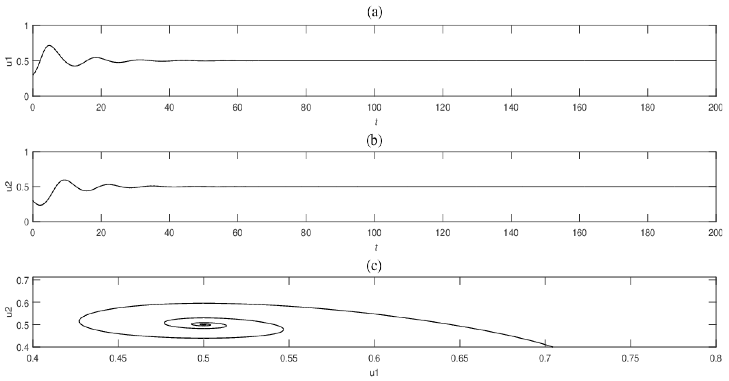
Firstly, we use numerical simulations to illustrate the stability of the coexistence equilibrium points in the ODE system. We choose appropriate parameters in ODE system (7), and the two populations tend to be stable and coexist, as shown in Figure 1. For PDE system (5) with cross-diffusion, Figure 2 and Figure 3 show the relation between the real part of the eigenvalue λ and cross-diffusion coefficient c 3 or Allee effect constant σ . Due to Theorem 3, we state that when the real part of the maximum eigenvalue is greater than zero, the system equilibrium point will become unstable. 
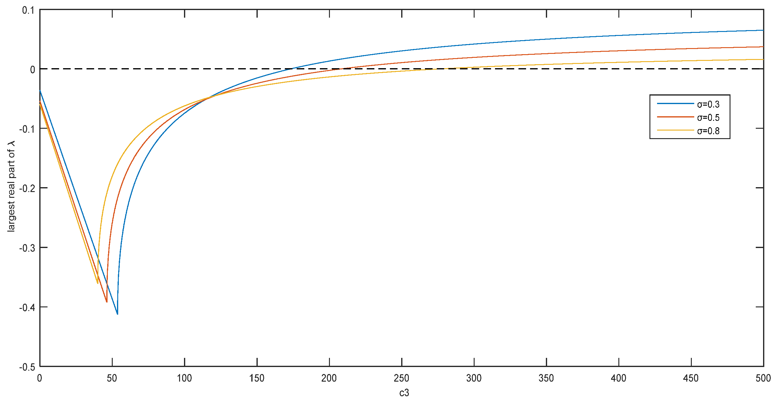
Figure 2 shows the real part of the eigenvalues λ as a function of c 3 , and the cross-diffusion coefficient can affect the stability of the coexistence equilibrium points. When σ is 0.3, 0.5, or 0.8, the critical value of c 3 is 173.4, 208.4, or 277.3, respectively. For different σ , the critical value of c 3 is different. It can be concluded that the Allee effect constant also affects the stability of the coexistence equilibrium points. 
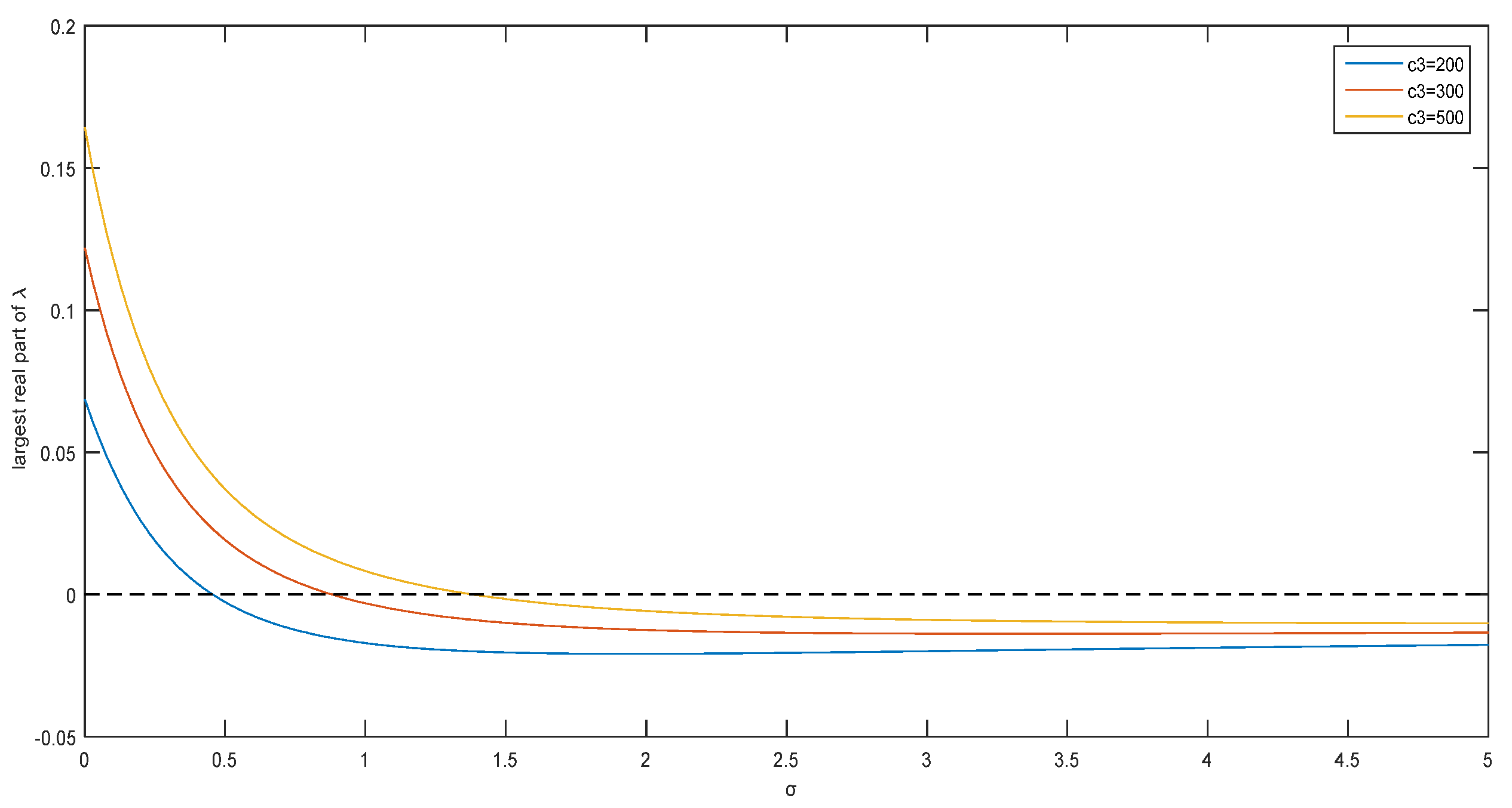
Figure 3 shows that when the parameter c 3 is fixed, there is also a critical value for σ to induce the instability of coexistence equilibrium points of the system (5). When c 3 is 200, 300, or 500, the critical value of σ is 0.455, 0.882, or 1.385, respectively.
Next, the numerical simulations show that the system (11) with self-diffusion does not form a space pattern, and in the PDE system (5) with cross-diffusion, the system will form a spatial stationary pattern. We suppose the area of system (5) is a rectangular area Ω = [ 0 , L ] × [ 0 , L ] R 2 with L = 200 . Additionally, we study the system (5) in a domain with 200 × 200 stations using the simple Euler method with the Laplacian operator in a discrete grid of lattice points denoted by ( p , q ) ,   p = 1 , 2 N , q = 1 , 2 N . The form is
Δ k | ( i , j ) = 1 s 2 ( k ( p 1 , q ) + k ( p + 1 , q ) ) + k ( p , q 1 ) + k ( p , q + 1 ) 4 k ( p , q )   ,
s is the lattice constant. Let s = 1 . When ( p , q ) is on the left boundary, we define k ( p , 0 ) k ( p , 1 ) . When ( p , q ) is on the right boundary, we define k ( p , N + 1 ) k ( p , N ) . When ( p , q ) is on the upper boundary, we define k ( 0 , q ) k ( 1 , q ) . When ( p , q ) is on the lower boundary, we define k ( N + 1 , q ) k ( N , q ) . This indicates that the population flux across the border is zero.
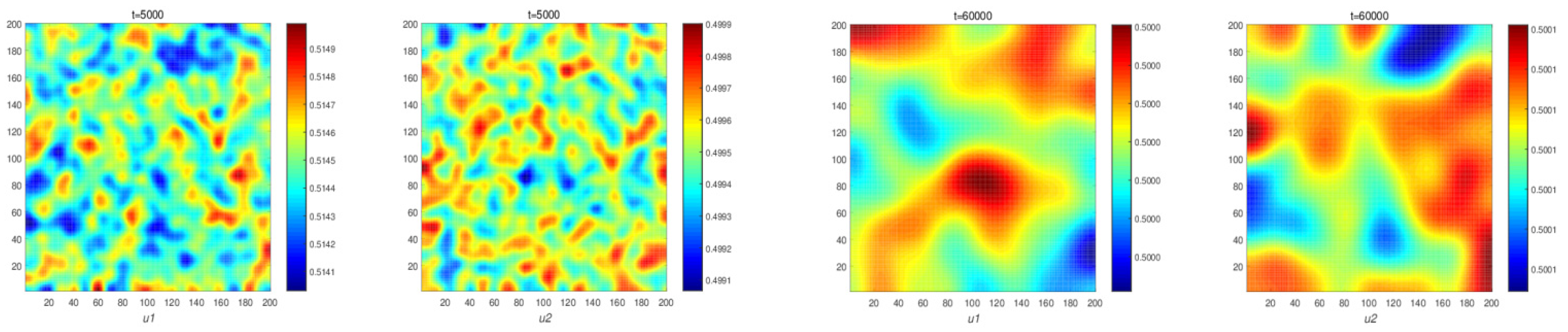
Then, we choose the Allee effect constant that makes system (11) with self-diffusion stable. Figure 4 illustrates changes in the population density of prey and predators in system (11). It can be seen that system (11) does not form a space pattern. This verifies the result of Theorem 4 in Section 4, and it shows that the system with self-diffusion cannot induce a space pattern. Next, we select suitable parameters to generate the spatial patterns. They satisfy condition (8) and (13). 
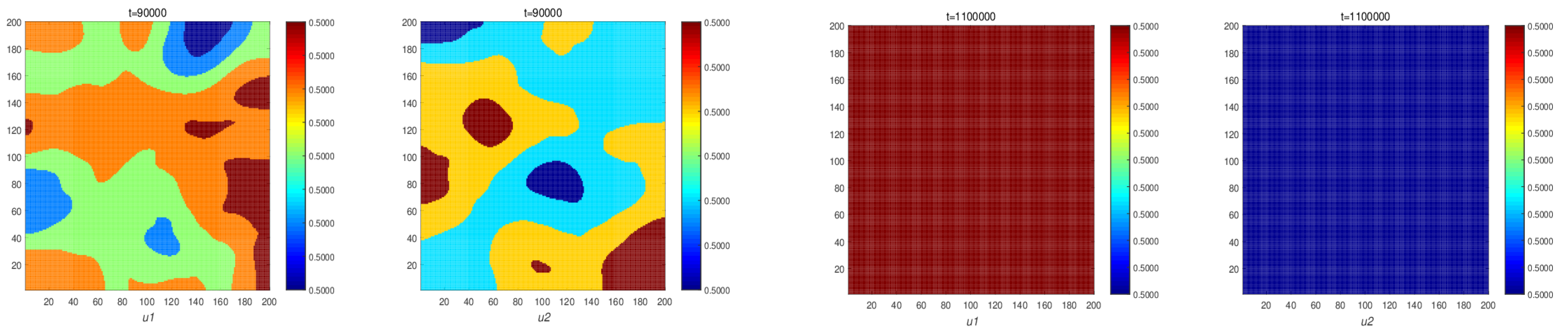
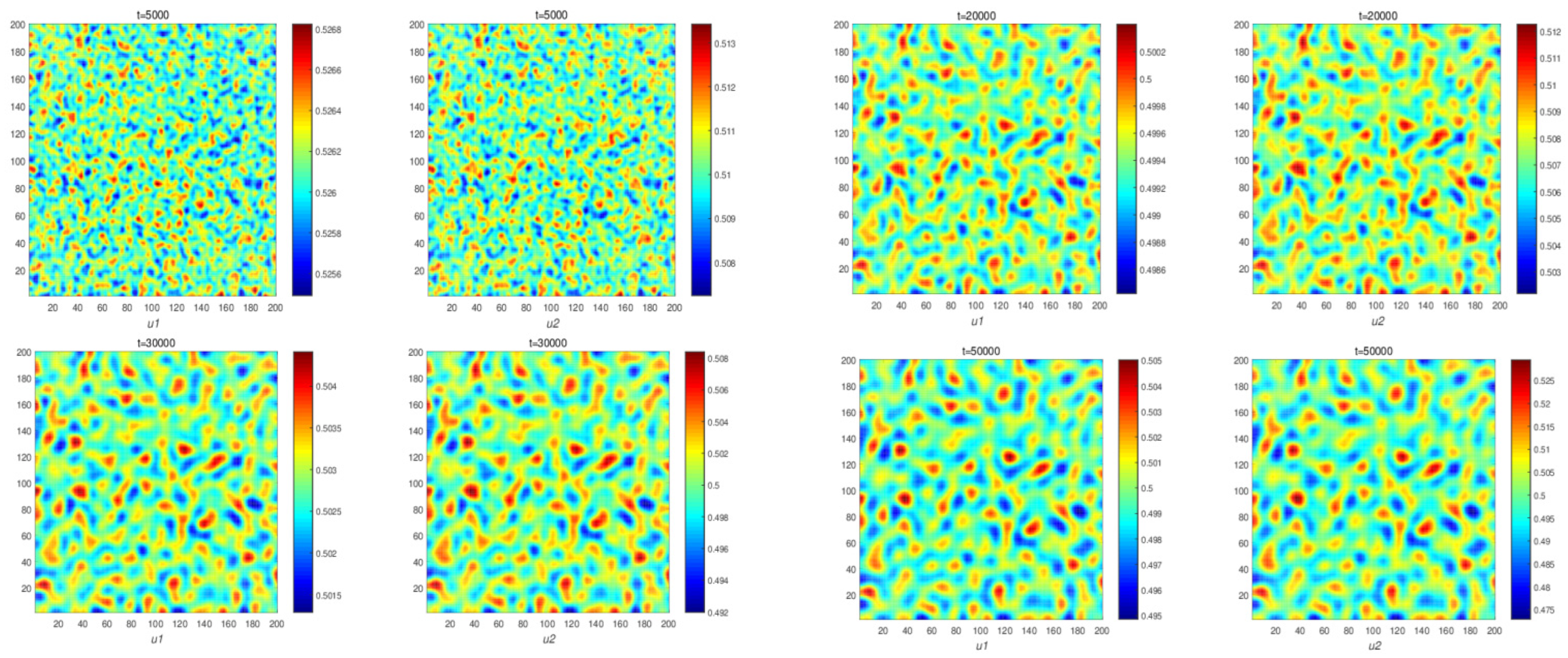
Figure 5 shows the spatial pattern for system (5). When the time reaches 30,000, the spatial pattern is unchanged. So, as time increases, it shows that the system forms a spatial stationary pattern. Numerical simulations illustrate our theoretical results of Theorem 5.

6. Concluding Remarks

In our article, we studied a spatial predator–prey model with the Allee effect and nonlinear reaction cross-diffusion to research the Turing instability and pattern formation caused by cross-diffusion. Moreover, the Allee effect produces considerable influence on the stability of the system.
For ODE system (7) and system (11) with self-diffusion, if the Allee effect constant is within the stable range, the coexistence equilibrium of the model is asymptotically stable (Theorem 1 and Theorem 2), which means that two populations will tend to be stable and coexist in ODE system (7) (see Figure 1). For system (5) with nonlinear cross-diffusion, the system will induce Turing instability when the cross-diffusion coefficient c 3 is big enough and satisfies conditions (8) and (13) (Theorem 3). Figure 2 shows the relationship between the real part of the maximum eigenvalue λ and the cross-diffusion coefficient c 3 . When c 3 is big enough, the real part of the maximum eigenvalue is positive, that is, the system is unstable. Figure 3 shows the relationship between the real part of the maximum eigenvalue λ and the Allee effect constant. The critical value of c 3 increases with the value of the Allee effect constant. Thus, the Allee effect also affects the stability of system (5).
Furthermore, in Theorem 4, if the Allee effect constant is within the stable range, we prove that the model has a constant solution for system (11) with self-diffusion. Choosing appropriate parameters, numerical simulation shows the spatial patterns. It shows predator and prey densities do not change over time, and finally, it reaches the stationary uniform solution. The system cannot generate spatial patterns (see Figure 4). When the cross-diffusion is present, we prove reaction system (5) could produce nonconstant, positive, steady-state solutions (Theorem 5). Figure 5 shows stationary patterns in system (5). It shows that a predator–prey ecosystem with self-diffusion does not form spatial patterns, while in an ecosystem with cross-diffusion, the population forms spatial patterns.
In our model, the Allee effect and the nonlinear cross-diffusion term were introduced together to study the stability and spatial patterns of the system. Biologically, due to the fact that the impacts of the Allee effect on different predator–prey systems are quite different, under the Allee effect, a system with self-diffusion will change its stability at the equilibrium point. Meanwhile, the mobility of a population is largely influenced by the abundance of the presence or absence of another population. The uniform steady state of a self-diffusion system is stable under nonuniform perturbations, but because of cross-diffusion, it loses its stability and produces various modes. This explains the destabilizing effect of nonlinear cross-diffusion.

Author Contributions

Writing—original draft, software, writing—review and editing, Y.S.; methodology, writing—review and editing, software, Y.M.; writing—review and editing, supervision, X.X. All authors have read and agreed to the published version of the manuscript.

Funding

This work is jointly supported by the National traditional Medicine Clinical Research Base Business Construction Special Topics (JDZX2015299) and the Fundamental Research Funds for the Central University FRF-BR-16-019A.

Institutional Review Board Statement

Not applicable.

Informed Consent Statement

Not applicable.

Data Availability Statement

Not applicable.

Conflicts of Interest

The authors declare no conflict of interest.

References

  1. Allee, W.C. Animal Aggregations: A Study in General Sociology; University of Chicago Press: Chicago, IL, USA, 1931. [Google Scholar]
  2. Wang, J.; Shi, J.; Wei, J. Predator-prey system with strong Allee effect in prey. J. Math. Biol. 2011, 62, 291–331. [Google Scholar] [CrossRef] [PubMed]
  3. Yun, K.; Yakubu, A.A. Weak Allee effects and species coexistence. Nonlinear Anal. 2011, 12, 3329–3345. [Google Scholar] [CrossRef]
  4. Wang, M.; Kot, M. Speeds of invasion in a model with strong or weak Allee effects. Math. Biosci. 2001, 171, 83–97. [Google Scholar] [CrossRef]
  5. Wang, W.; Zhang, Y.; Liu, C. Analysis of a discrete-time predator–prey system with Allee effect. Ecol. Complex. 2011, 8, 81–85. [Google Scholar] [CrossRef]
  6. Manna, K.; Banerjee, M. Stationary, non-stationary and invasive patterns for a prey-predator system with additive Allee effect in prey growth. Ecol. Complex. 2018, 36, 206–217. [Google Scholar] [CrossRef]
  7. Rao, F.; Kang, Y. The complex dynamics of a diffusive prey–predator model with an Allee effect in prey. Ecol. Complex. 2016, 28, 123–144. [Google Scholar] [CrossRef]
  8. Yao, S.; Ma, Z.; Cheng, Z. Pattern formation of a diffusive predator–prey model with strong Allee effect and nonconstant death rate. Phys. A 2019, 527, 121350. [Google Scholar] [CrossRef]
  9. Ni, W.; Wang, M. Dynamics and patterns of a diffusive Leslie-Gower prey-predator model with strong Allee effect in prey. J. Differ. Equ. 2016, 261, 4244–4274. [Google Scholar] [CrossRef]
  10. Ni, W.; Wang, M. Dynamical properties of a Leslie-Gower prey-predator model with strong Allee effect in prey. Discrete Contin. Dyn. Syst. Ser. B 2017, 22, 3409–3420. [Google Scholar] [CrossRef] [Green Version]
  11. Alan, J.T. Predator-prey models with component Allee effect for predator reproduction. J. Math. Biol. 2015, 71, 1325–1352. [Google Scholar] [CrossRef]
  12. Wang, J.; Shi, J.; Wei, J. Dynamics and pattern formation in a diffusive predator–prey system with strong Allee. J. Differ. Equ. 2011, 251, 1276–1304. [Google Scholar] [CrossRef] [Green Version]
  13. Landge, A.N.; Jordan, B.M.; Diego, X.; Müller, P. Pattern formation mechanisms of self-organizing reaction-diffusion systems. Dev. Biol. 2020, 460, 2–11. [Google Scholar] [CrossRef] [PubMed]
  14. Iqbal, N.; Karaca, Y. Complex fractional-order HIV diffusion model based on amplitude equations with turing patterns and turing instability. Fractals 2021, 29, 2140013. [Google Scholar] [CrossRef]
  15. Kim, H.; Yun, A.; Yoon, S.; Lee, C.; Park, J.; Kim, J. Pattern formation in reaction–diffusion systems on evolving surfaces. Comput. Math. Appl. 2020, 80, 2019–2028. [Google Scholar] [CrossRef]
  16. Peng, Y.; Ling, H. Pattern formation in a ratio-dependent predator-prey model with cross-diffusion. Appl. Math. Comput. 2018, 331, 307–318. [Google Scholar] [CrossRef]
  17. Mansouri, D.; Abdelmalek, S.; Bendoukha, S. Bifurcations and pattern formation in a generalized Lengyel-Epstein reaction-diffusion model. Chaos Soliton. Fract. 2020, 132, 109579. [Google Scholar] [CrossRef]
  18. Paquin-Lefebvre, F.; Xu, B.; DiPietro, K.L.; Lindsay, A.E.; Jilkine, A. Pattern formation in a coupled membrane-bulk reaction-diffusion model for intracellular polarization and oscillations. J. Theor. Biol. 2020, 497, 110242. [Google Scholar] [CrossRef] [Green Version]
  19. Poole, T.; Dunstone, N. Underwater predatory behaviour of the American mink Mustela vison. J. Zool. 1975, 178, 395–412. [Google Scholar] [CrossRef]
  20. Freund, R.; Littell, R. SAS for Linear Models: A Guide to the ANOVA and GEM Procedures; SAS Institute Inc.: Cary, NC, USA, 1986; p. 231. [Google Scholar]
  21. Magurran, A.; Pitcher, T. Foraging, timidity and shoal size in minnows and goldfish. Behav. Ecol. Sociobiol. 1983, 12, 142–152. [Google Scholar] [CrossRef]
  22. Magurran, A.; Pitcher, T. UForaging, Provenance, shoal size and the sociobiology of predator-evasion behavisur in minnow shoals. Roc. R. Soc. Lond. B Biol. Sci. 1987, 229, 439–466. [Google Scholar]
  23. Pitcher, T.; Magurran, A.; Allan, J. Size-segregative behaviour in minnow shoals. J. Fish Biol. 1986, 29, 83–95. [Google Scholar] [CrossRef]
  24. Street, N.; Magurran, A.; Pitcher, T. The effects of increasing shoal size on handling time in goldfish Carassius aurutus. J. Fish Biol. 1984, 25, 561–566. [Google Scholar] [CrossRef]
  25. Pullian, H.; Caraco, T. Living in groups: Is there an optimal group size? In Behaviouml Ecology. An Evolutionary Approach, 2nd ed.; Krebs, J.R., Davies, N.B., Eds.; Blackwell Scientific Publications: Oxford, UK, 1984. [Google Scholar]
  26. Lei, C.; Zhang, G.; Zhou, J. Pattern formation of a biomass-water reaction-diffusion model. Appl. Math. Lett. 2022, 123, 107605. [Google Scholar] [CrossRef]
  27. Wang, G.; Liang, X.; Wang, F. The competitive dynamics of populations subject to an Allee effect. Ecol. Modell. 1999, 124, 183–192. [Google Scholar] [CrossRef]
  28. Capone, F.; Carfora, M.F.; De Luca, R.; Torcicollo, I. Turing patterns in a reaction–diffusion system modeling hunting cooperation. Math. Comput. Simul. 2019, 165, 172–180. [Google Scholar] [CrossRef]
  29. Fu, S.; He, X.; Zhang, L.; Wen, Z. Turing patterns and spatiotemporal patterns in a tritrophic food chain model with diffusion. Nonlinear Anal. Real World Appl. 2021, 59, 103260. [Google Scholar] [CrossRef]
  30. Chakraborty, B.; Bairagi, N. Complexity in a prey-predator model with prey refuge and diffusion. Ecol. Complex. 2019, 37, 11–23. [Google Scholar] [CrossRef]
  31. De Oliveira Vilaca, L.M.; Gómez-Vargas, B.; Kumar, S.; Ruiz-Baier, R.; Verma, N. Stability analysis for a new model of multi-species convection-diffusion-reaction in poroelastic tissue. Appl. Math. Model. 2020, 84, 425–446. [Google Scholar] [CrossRef]
  32. Han, R.; Dai, B. Spatiotemporal pattern formation and selection induced bynonlinear cross-diffusion in a toxic-phytoplankton-zooplanktonmodel with Allee effect. Nonlinear Anal. Real World Appl. 2019, 45, 822–853. [Google Scholar] [CrossRef]
  33. Mukherjee, N.; Ghorai, S.; Banerjee, M. Effects of density dependent cross-diffusion on the chaotic patterns in a ratio-dependent prey-predator model. Ecol. Complex. 2018, 36, 276–289. [Google Scholar] [CrossRef]
  34. Yao, S.; Ma, Z.; Yue, J. Bistability and Turing pattern induced by cross fraction diffusion in a predator-prey model. Phys. A. 2018, 509, 982–988. [Google Scholar] [CrossRef]
  35. Iqbal, N.; Wu, R. Turing patterns induced by cross-diffusion in a 2D domain with strong Allee effect. Comptes Rendus Mathematique. 2019, 357, 863–877. [Google Scholar] [CrossRef]
  36. Banerjee, M.; Ghorai, S.; Mukherjee, N. Study of cross-diffusion induced Turing patterns in a ratio-dependent prey-predator model via amplitude equations. Appl. Math. Model. 2018, 55, 383–399. [Google Scholar] [CrossRef]
  37. Ghorai, S.; Poria, S. Turing patterns induced by cross-diffusion in a predator-prey system in presence of habitat complexity. Chaos Soliton. Fract. 2016, 91, 421–429. [Google Scholar] [CrossRef]
  38. Rahim, H.; Iqbal, N.; Cong, C.; Ding, Z. Pattern selection of three components Gray-Scott model. J. Phys. Conf. Ser. 2019, 1324, 012012. [Google Scholar] [CrossRef]
  39. Lacitignola, D.; Sgura, I. Turing-Hopf patterns in a morphochemical model for electrodeposition with cross-diffusion. Appl. Eng. Sci. 2021, 5, 100034. [Google Scholar] [CrossRef]
  40. Currò, C.; Valenti, G. Pattern formation in hyperbolic models with cross-diffusion: Theory and applications. Phys. D 2021, 418, 132846. [Google Scholar] [CrossRef]
  41. Iqbala, N.; Wub, R.; Mohammed, W.W. Pattern formation induced by fractional cross-diffusion in a 3-speciesfood chain model with harvesting. Math. Comput. Simul. 2021, 188, 102–119. [Google Scholar] [CrossRef]
  42. Turing, A.M. The chemical basis of morphogenesis. Philos. Trans. R. Soc. Lond. B 1952, 237, 37–72. [Google Scholar] [CrossRef]
  43. Pang, P.Y.H.; Wang, M. Strategy and stationary pattern in a three-species predator-prey model. J. Differ. Equ. 2004, 200, 245–273. [Google Scholar] [CrossRef] [Green Version]
  44. Lv, Y.; Yuan, R.; Pei, Y. Turing pattern formation in a three species model with generalist predator and cross-diffusion. Nonlinear Anal. 2013, 85, 214–232. [Google Scholar] [CrossRef]
  45. Tian, C.; Ling, Z.; Lin, Z. Turing pattern formation in a predator-prey-mutualist system. Nonlinear Anal. Real World Appl. 2011, 12, 3224–3237. [Google Scholar] [CrossRef]
Figure 1. Dynamics curves of prey (a), predator (b), and phase diagram (c) of system (7). Parameters are σ = 0.3 , β = 0.1 , δ = 0.5 , ω = 2 , c 5 = 0.5 .
Mathematics 10 01500 g001
Figure 2. The relation between the real part of the eigenvalue λ and c 3 . The blue, red, and yellow lines correspond to curve lines with σ = 0.3 ,   σ = 0.5 ,   σ = 0.8 , respectively. Parameters are: β = 0.1 , δ = 0.5 ,   ω = 2 ,   c 5 = 0.5 , c 1 = 0.01 ,   c 2 = 0.01 ,   c 4 = 100 .
Mathematics 10 01500 g002
Figure 3. The relation between the real part of the eigenvalue λ and σ . The blue, red, and yellow lines correspond to curve lines with c 3 = 200 ,   c 3 = 300 ,   c 3 = 500 , respectively. Parameters are: β = 0.1 , δ = 0.5 ,   ω = 2 ,   c 5 = 0.5 , c 1 = 0.01 ,   c 2 = 0.01 ,   c 4 = 100 .
Mathematics 10 01500 g003
Figure 4. Spatial patterns of the time evolution of the species density of prey population and predator population at different instants with σ = 0.3 ,   β = 0.1 ,   δ = 0.5 ,   ω = 2 ,   c 5 = 0 ,   c 1 = 1 ,   c 2 = 2 ,   c 3 = 1 ,   c 4 = 0 . Moments: t = 5000; t = 60,000; t = 90,000 t = 110,000. ( u 1 ( x ) and u 2 ( x ) are the population densities of prey and predator).
Mathematics 10 01500 g004aMathematics 10 01500 g004b
Figure 5. Spatial patterns of the time evolution of the species density of prey population and predator population at different instants with σ = 0.3 ,   β = 0.1 ,   δ = 0.5 ,   ω = 2 ,   c 5 = 0.5 ,   c 1 = 0.01 ,   c 2 = 0.01 ,   c 3 = 200 ,   c 4 = 10 . Moments: t = 5000; t = 20,000; t = 30,000; t = 50,000.( u 1 ( x ) and u 2 ( x ) are the population densities of prey and predator).
Mathematics 10 01500 g005
Publisher’s Note: MDPI stays neutral with regard to jurisdictional claims in published maps and institutional affiliations.

