
Exploring Radial Kernel on the Novel Forced SEYNHRV-S Model to Capture the Second Wave of COVID-19 Spread and the Variable Transmission Rate


Abstract
:1. Introduction
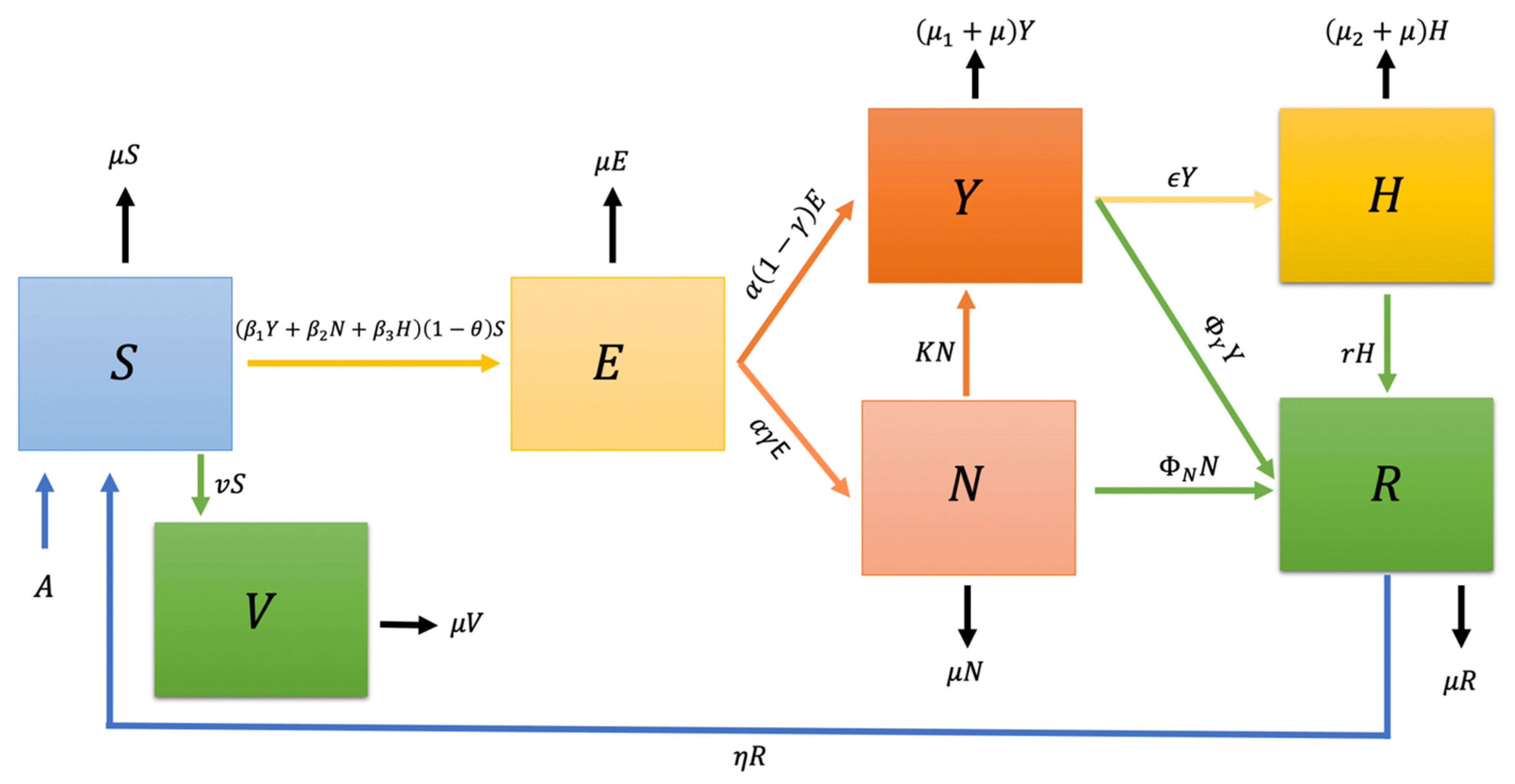
2. The Model
3. Mathematical Analysis
- (i)
- If , then the other unknown functions are non-negative at . Hence, we obtained the following from the first differential equation in Equation (1):which tells us that we have , such that is strictly monotone, increasing on .
- (ii)
- If , then the rest of the state variables are non-negative at ; Then, we have:There are two cases:
- (1)
- If at least one of the state variable is not zero, then:which is a contradiction similar to (i).
- (2)
- If all state variables are zero, then:
- (iii)
- If , and , then:which is a contradiction similar to (i).
- (iv)
- If , , , and , then:which is a contradiction similar to (i). Similarly, , , and lead to a contradiction. Thus, and are all positive for .
Radial Kernels (Functions)
- The Gaussian (GA): ;
- The Laguerre–Gaussian (LG): ;
- The inverse quadratic (IQ): ;
- The generalized inverse multiquadric (GIMQ):
4. Forced SEYNHRV-S Model
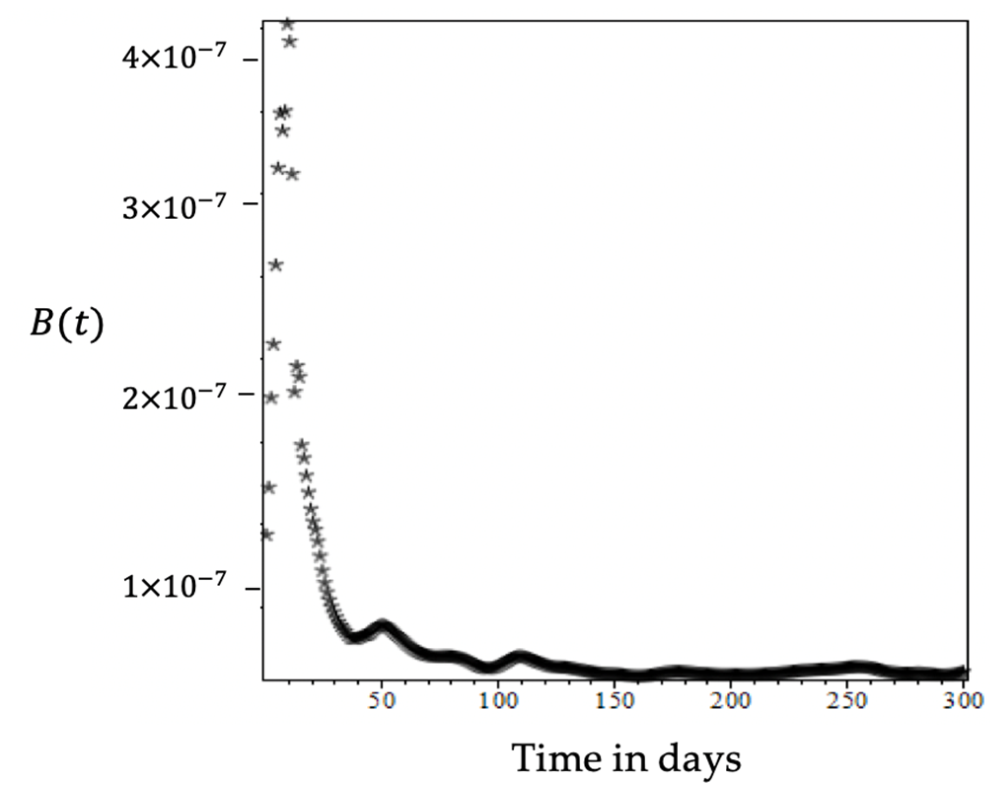
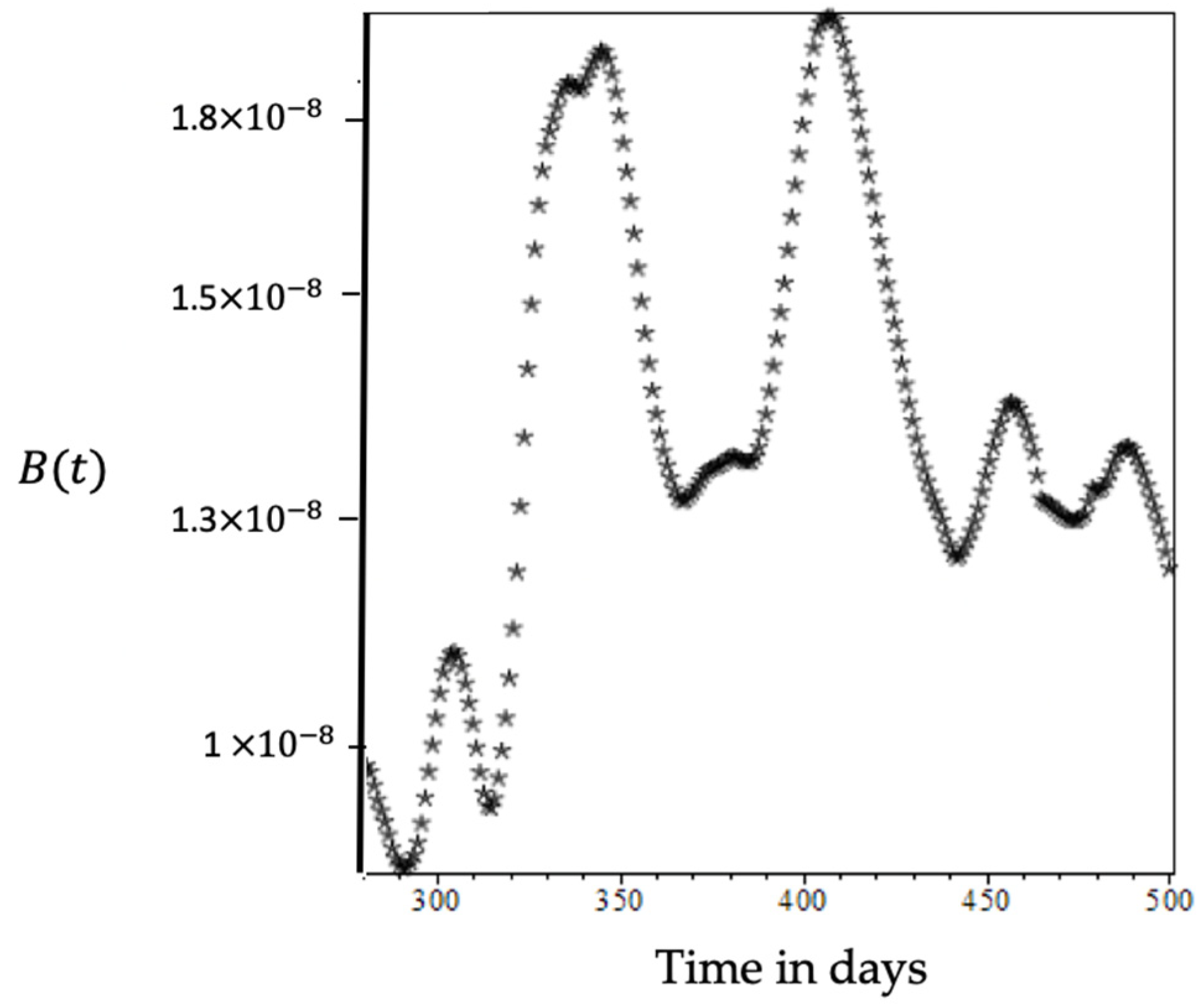
Driving the Transmission Rate from the Infected Population and a Numerical Solution
- (i)
- The method is stable;
- (ii)
- The differences method is convergent if it is equivalent to for all ;
- (iii)
- If the function of exists, then for each, j = 1, 2, …, N, the local truncation error satisfies whenever , then:
5. Methodology
Model Calibration
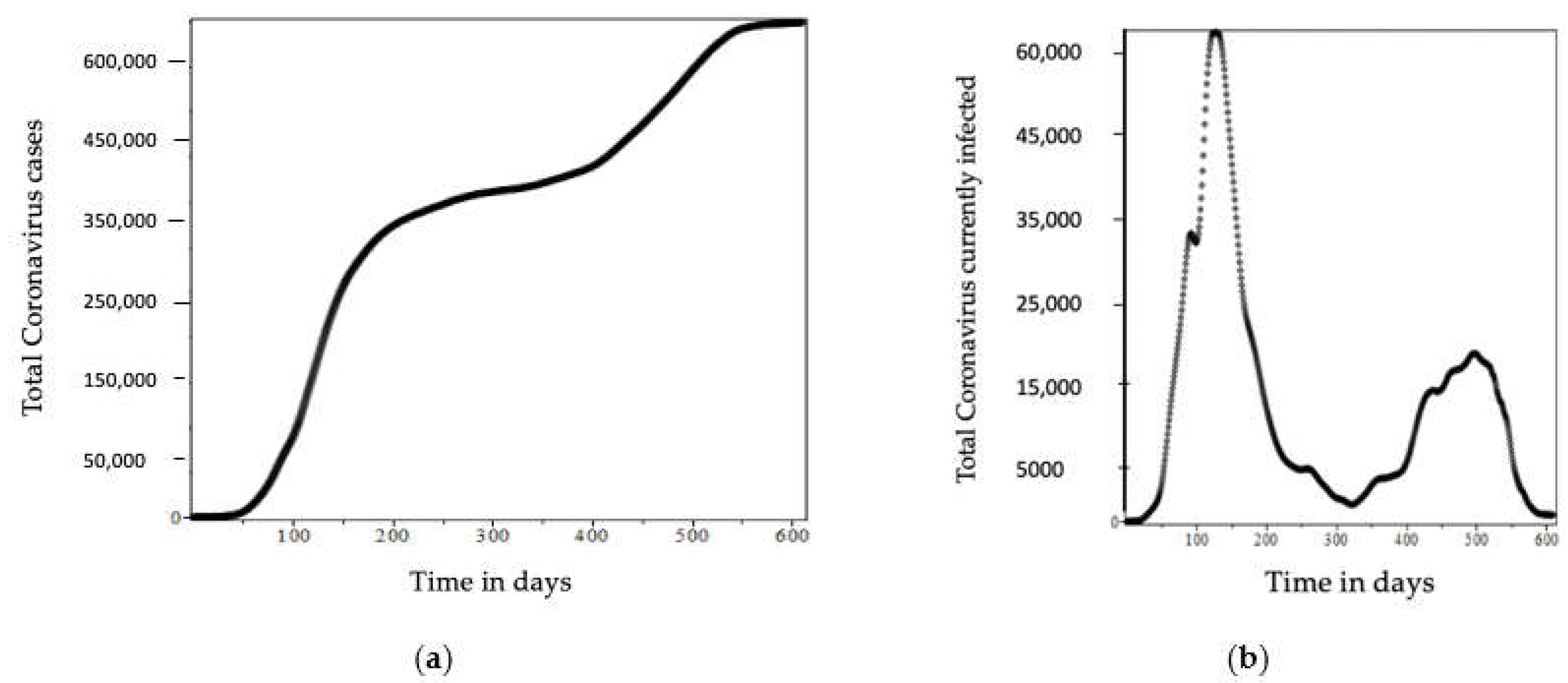
6. Results
7. Discussion
Author Contributions
Funding
Institutional Review Board Statement
Informed Consent Statement
Data Availability Statement
Acknowledgments
Conflicts of Interest
References
- WHO. Coronavirus Disease (COVID-19) Pandemic. Available online: https://www.who.int/emergencies/diseases/novel-coronavirus-2019 (accessed on 17 November 2021).
- Cao, L.; Liu, Q. COVID-19 Modeling: A Review. arXiv 2021, arXiv:2104.12556. Available online: https://arxiv.org/abs/2104.12556 (accessed on 3 November 2021).
- Kermack, W.O.; McKendrick, A.G. A contribution to the mathematical theory of epidemics. Proc. R. Soc. A 1927, 115, 700–721. [Google Scholar]
- Ivorra, B.; Ferrández, M.R.; Vela-Pérez, M.; Ramos, A.M. Mathematical modeling of the spread of the coronavirus disease 2019 (COVID-19) taking into account the undetected infections. The case of China. Commun. Nonlinear Sci. Numer. Simul. 2020, 88, 105303. [Google Scholar] [CrossRef] [PubMed]
- Giordano, G.; Colaneri, M.; Di Filippo, A.; Blanchini, F.; Bolzern, P.; Nicolao, G.D.; Sacchi, P.; Colaneri, P.; Bruno, R. Modeling vaccination rollouts, SARS-CoV-2 variants and the requirement for non-pharmaceutical interventions in Italy. Nat. Med. 2021, 27, 993–998. [Google Scholar] [CrossRef] [PubMed]
- Antonini, C.; Calandrini, S.; Bianconi, F. A Modeling Study on Vaccination and Spread of SARS-CoV-2 Variants in Italy. Vaccine 2021, 9, 915. [Google Scholar] [CrossRef] [PubMed]
- Yang, H.M.; Lombardi, L.S., Jr.; Castro, F.F.M.; Yang, A.C. Mathematical modeling of the transmission of SARS-CoV-2—Evaluating the impact of isolation in São Paulo State (Brazil) and lockdown in Spain associated with protective measures on the epidemic of COViD-19. PLoS ONE 2021, 16, e0252271. [Google Scholar] [CrossRef] [PubMed]
- Ramos, M.R.; Vela-Pérez, A.M.; Ferrández, M.; Kubik, A.B.; Ivorra, B. Modeling the impact of SARS-CoV-2 variants and vaccines on the spread of COVID-19. Commun. Nonlinear Sci. Numer. Simul. 2021, 102, 105937. [Google Scholar] [CrossRef] [PubMed]
- Moore, S.; Hill, E.M.; Tildesley, M.J.; Dyson, L.; Keeling, M.J. Vaccination and non-pharmaceutical interventions for COVID-19: A mathematical modelling study. Lancet Infect. Dis. 2021, 21, 793–802. [Google Scholar] [CrossRef]
- Mancuso, M.; Eikenberry, S.E.; Gumel, A.B. Will Vaccine-Derived Protective Immunity Curtail COVID-19 Variants in the US? Infect. Dis. Model. 2021, 6, 1110–1134. [Google Scholar] [CrossRef] [PubMed]
- Ngonghala, C.N.; Knitter, J.R.; Marinacci, L.; Bonds, M.H.; Gumel, A.B. Assessing the impact of widespread respirator use in curtailing COVID-19 transmission in the USA. R. Soc. Open Sci. 2021, 8, 210699. [Google Scholar] [CrossRef] [PubMed]
- Asamoah, J.K.K.; Jin, Z.; Sun, G.-Q.; Seidu, B.; Yankson, E.; Abidemi, A.; Oduro, F.; Moore, S.E.; Okyere, E. Sensitivity assessment and optimal economic evaluation of a new COVID-19 compartmental epidemic model with control interventions. Chaos Solitons Fractals 2021, 146, 110885. [Google Scholar] [CrossRef] [PubMed]
- Asamoah, J.K.K.; Owusu, M.A.; Jin, Z.; Oduro, F.; Abidemi, A.; Gyasi, E.O. Global stability and cost-effectiveness analysis of COVID-19 considering the impact of the environment: Using data from Ghana. Chaos Solitons Fractals 2020, 140, 110103. [Google Scholar] [CrossRef] [PubMed]
- Demongeot, J.; Flet-Berliac, Y.; Seligmann, H. Temperature decreases spread parameters of the new COVID-19 case dynamics. Biology 2020, 9, 94. [Google Scholar] [CrossRef] [PubMed]
- Alshammari, F.S. A Mathematical Model to Investigate the Transmission of COVID-19 in the Kingdom of Saudi Arabia. Comput. Math. Methods Med. 2020, 2020, 9136157. [Google Scholar] [CrossRef] [PubMed]
- Buhmann, M.D. Radial basis functions: Theory and implementations. In Cambridge Monographs on Applied and Computational Mathematics; Cambridge University Press: Cambridge, UK, 2003; Volume 12. [Google Scholar]
- Wendland, H. Scattered Data Approximation. In Cambridge Monographs on Applied and Computational Mathematics; Cambridge University Press: Cambridge, UK, 2005. [Google Scholar]
- Schaback, R. A Practical Guide to Radial Basis Functions. 2007. Available online: num.math.uni-goettingen.de/schaback/teaching/sc.pdf (accessed on 8 December 2021).
- Chalkiadakis, I.; Yan, H.; Peters, G.W.; Shevchenko, P.V. Infection rate models for COVID-19: Model risk and public health news sentiment exposure adjustments. PLoS ONE 2021, 16, e0253381. [Google Scholar] [CrossRef]
- Corsaro, C.; Sturniolo, A.; Fazio, E. Gaussian Parameters Correlate with the Spread of COVID-19 Pandemic: The Italian Case. Appl. Sci. 2021, 11, 6119. [Google Scholar] [CrossRef]
- Pollicott, M.; Wang, H.; Weiss, H. Extracting the time dependent transmission rate from infection data via solution of an inverse ODE problem. J. Biol. Dyn. 2012, 6, 509–523. [Google Scholar] [CrossRef] [PubMed]
- Ramezani, S.B.; Amirlatifi, A.; Rahimi, S. A novel compartmental model to capture the nonlinear trend of COVID-19. Comput. Biol. Med. 2021, 134, 104421. [Google Scholar] [CrossRef] [PubMed]
- Gear, C.W. Numerical Initial-Value Problems in Ordinary Differential Equations; Prentice-Hall: Englewood Cliffs, NJ, USA, 1971; Volume 253, pp. 57–58. [Google Scholar]
- General Authority of Statistics, Kingdom of Saudi Arabia. Available online: https://www.stats.gov.sa/en (accessed on 19 April 2020).


| Parameter | Description | Reported Value | Experimental Value |
|---|---|---|---|
| Transmission rate of the asymptomatic population | (1 × 10⁸, 2 × 10⁶) | (0, 0.025) | |
| Transmission rate of the hospitalized population | (1 × 10⁹, 2 × 10⁷) | (0, 0.0025) | |
| Natural death rate 3.6593 × 10⁻⁵ (Saudi Arabia) | |||
| Incubation period | (1/14, 1/21) | (1/8, 1/6) | |
| Fraction of the individuals ultimately becoming infected | |||
| Mean symptomatic infectious period | (14, 21) | (8, 16) | |
| Mean symptomatic infectious period | (14, 21) | (8, 16) | |
| Vaccination rate—data taken from Saudi Arabia | |||
| Rate of recovered individuals losing their immunity and returning to | |||
| Rate of symptomatic individuals becoming hospitalized | (0.1, 0.5) | (0.01, 1) | |
| K | Rate of asymptomatic individuals becoming symptomatic | (0.05, 0.5) | (0.01, 1) |
| Rate of recovered individuals becoming hospitalized patients | (0.05, 0.5) | (0.01, 1) | |
| Death rate of hospitalized patients | (0.05, 0.5) | (0.01, 1) | |
Publisher’s Note: MDPI stays neutral with regard to jurisdictional claims in published maps and institutional affiliations. |
© 2022 by the authors. Licensee MDPI, Basel, Switzerland. This article is an open access article distributed under the terms and conditions of the Creative Commons Attribution (CC BY) license (https://creativecommons.org/licenses/by/4.0/).
Share and Cite
Alshammari, F.S.; Tezcan, E.A. Exploring Radial Kernel on the Novel Forced SEYNHRV-S Model to Capture the Second Wave of COVID-19 Spread and the Variable Transmission Rate. Mathematics 2022, 10, 1501. https://doi.org/10.3390/math10091501
Alshammari FS, Tezcan EA. Exploring Radial Kernel on the Novel Forced SEYNHRV-S Model to Capture the Second Wave of COVID-19 Spread and the Variable Transmission Rate. Mathematics. 2022; 10(9):1501. https://doi.org/10.3390/math10091501
Chicago/Turabian StyleAlshammari, Fehaid Salem, and Ezgi Akyildiz Tezcan. 2022. "Exploring Radial Kernel on the Novel Forced SEYNHRV-S Model to Capture the Second Wave of COVID-19 Spread and the Variable Transmission Rate" Mathematics 10, no. 9: 1501. https://doi.org/10.3390/math10091501