
Algorithmic Strategies for Precious Metals Price Forecasting


Department of Management, Western Galilee Academic College, P.O. Box 2125, Acre 2412101, Israel
Mathematics 2022, 10(7), 1134; https://doi.org/10.3390/math10071134
Submission received: 24 February 2022
/
Revised: 18 March 2022
/
Accepted: 30 March 2022
/
Published: 1 April 2022
(This article belongs to the Special Issue Probability, Stochastic Processes and Optimization)
Abstract
:This research is the first attempt to create machine learning (ML) algorithmic systems that would be able to automatically trade precious metals. The algorithm uses three forecast methodologies: linear regression (LR), Darvas boxes (DB), and Bollinger bands (BB). Our data consists of 20 years of daily price data concerning five precious metals futures: gold, silver, copper, platinum, and palladium. We found that all of the examined precious metals’ current daily returns are negatively autocorrelated to their former day’s returns and identified lagged interdependencies among the examined metals. Silver futures prices were found to be best forecasted by our systems, and platinum the worst. Moreover, our system better forecasts price-up trends than downtrends for all examined techniques and commodities. Linear regression was found to be the best technique to forecast silver and gold prices trends, while the Bollinger band technique best fits palladium forecasting.
1. Introduction
The use of artificial intelligence (AI) in financial assets price forecasting and trading has become more and more frequent as the amount and speed of the flow of new financial data increased dramatically. Algorithms are used to analyze simultaneous multi-sourced data. Those systems are developed by market experts and are usually applied to stocks and currencies markets. The following research develops and tests such an AI system and applies it to the precious metals’ futures market. Precious metals have always been perceived by investors as a hedging tool against inflation (see, for example, [1]) or stock market crashes. In the following research, we designed, optimized, and tested three algorithmic trading systems suitable for precious metal futures trading. Our long period of time data enables us to test the performance of our system over changing economic conditions. The technical analysis approach used here, commonly used by practitioners to trade stocks and foreign exchanges, relies on historical data for the sake of forecasting future prices. We used the particle swarm optimization (PSO) algorithm as our primary optimization tool because of its ability to handle multi-objective optimization simultaneously.
Many researchers have tried to prove the ability of such algorithmic trading systems to achieve abnormal returns for stocks, currencies, and indices. However, many researchers focus on stocks and foreign exchange and partly neglected commodity futures and especially precious metal futures. The following research aims to fill that gap with an insight into three algorithmic trading strategies that were programmed in accordance with the uniqueness of the precious metal financial markets. We use 20 years of daily futures data corresponding to five major precious metals, including gold, silver, copper, platinum, and palladium, to test three algorithmic trading strategies: linear regression (LR), Darvas boxes (DB), and Bollinger bands (BB). We followed [2], that concluded that LR and DB could help traders predict Bitcoin short-term price trends. Our 20 years of data were split into 10 years of training and optimization and 10 years of testing the trading results. We found that it is possible to forecast short-term price trends of precious metals. Silver futures prices were found to be best forecasted by our systems, and platinum was the worst. Our system better forecasts price-up trends than downtrends for all examined techniques and commodities. Linear regression was found to be the best technique to forecast silver and gold prices, while the Bollinger band technique best fits palladium forecasting.
2. Literature Review
Our system is based on pattern recognition which is a developing AI field that helps us to understand different chaotic phenomena. [3] argued that the applicability of Bayesian methods was greatly enhanced through the development of a range of approximate inference algorithms such as variational Bayes and expectation propagation. An important foundation for learning input–output mapping from a set of examples was presented by [4]. They developed a theoretical framework for the approximation method based on regularization networks that are closely related to pattern recognition. Their methodologies included task-dependent clustering and dimensionality reduction. Other researchers provided an understanding of the mathematical concepts behind forecasting methods that are based on probabilistic derivations. [5] provided a joint introduction to Gaussian processes (GP) and relevance vector machines (RVM-developed by [6]). They found that RVMs allow the choice of more general basis functions, whereas the behavior of predictive variance is generally counterintuitive. [7] examined the GP and RVM models and concluded that probabilistic models could produce predictive distributions instead of point predictions.
Most researchers that tried to explain precious metals prices have done so by linking the stock market to the precious metal market. [8] explained that precious metal futures have higher returns when investor sentiment is pessimistic rather than optimistic. [9] argued that the price of precious metals and their volatility are driven by shocks originating in the economic uncertainty and risk appetite of investors that prevail in the equity market. Other researchers focused on the interrelations between the prices of the leading precious metals. [10] showed that precious metals were strongly correlated with each other in the last decade. [11] documented that weekly changes in traders’ positions have a destabilizing impact on subsequent conditional volatility in gold, silver, and palladium futures markets.
Other researchers linked precious metals prices to each other and other commodities. [12] examined spillover effects among six commodity futures markets and found that both gold and silver are information transmitters to other commodity futures markets. [13] have examined the impact of oil price changes on precious metals prices. They identified the safe-haven nature of precious metals against an oil price drop.
Past researchers also attempted to construct AI systems to predict precious metals prices. [14] proposed a model that combines the adaptive neuro-fuzzy inference system and genetic algorithm. [15] discovered hidden patterns governing systems’ evolution. Unlike these attempts to predict precious metals prices, we designed algorithmic trading systems and tested their ability to predict precious metals prices.
3. Data and Methodologies
Our data consists of 20 years of daily data of open–closed, high–low prices of five precious metals futures. We used a lagged multi-dimension stepwise regression model to examine lagged correlations between the daily return of the examined precious metals, including autocorrelations, as described in Equation (1).
where: = the daily return of gold, silver copper, platinum, and palladium, is 1…3 days ago daily returns of gold, silver, copper, platinum, and palladium.
The results of this model enabled us to better understand short term autocorrelations of returns and lagged dependencies between the precious metals price movements and helped us design our trading systems.
3.1. Algorithmic Trading System
We designed our algorithmic trading system to report the actual trading results: net profit (NP), percent of profitable trades of all trades (PP), and the profit factor (PF). NP is the dollar value of the total net profit generated by the trading system, PP is the percentage number of winning trades out of the entire set of trades generated by the system, and PF is defined as gross profits divided by gross losses. We programmed three algorithmic systems based on three sophisticated trading technical tools and altered their configuration until we achieved maximum profitability in terms of NP and PF. The designed systems are based on three methodologies: linear regression, Darvas boxes, and Bollinger bands which are well-known technical formations that are commonly used to analyze investment opportunities for stock and currencies traders. We then optimized NP and PF by altering the setups behind our systems and splitting the system’s performance into long and short positions.
The complexity of our systems requires multi-objective optimization formulas. We selected particle swarm optimization (PSO), developed by Kennedy and Eberhart ([16,17]) as our primary optimization method. This methodology enabled us to train the system in the initial period and test it in the latter period. The 20 years of our examined period were split into two separate periods, 10 years of training and optimizing and 10 years of testing and reporting results. We started the process with a random trading setup that included the trading time frames and the various tools ingredients. Next, for each setup, we evaluated the desired fitness of the trading results to our predefined goals: Maximum NP, PF, and PP. We then compared each result to its former maximum and set a new maximum if needed. The process is described in Equation (2).
where Vid = the value of each setup, Rand = random number, Pid = the setups initial identification, and Pgd = the setups’ maximum identification.
V (1) i + 1,d = Vid + C1Rand × Pid − Xid + C2R and Pgd − Xid
X (2) i + 1,d = Xid + Vid
Last, we looped the process using Equation (3) until the highest multiple objectives were achieved.
3.2. Linear Regression Strategy
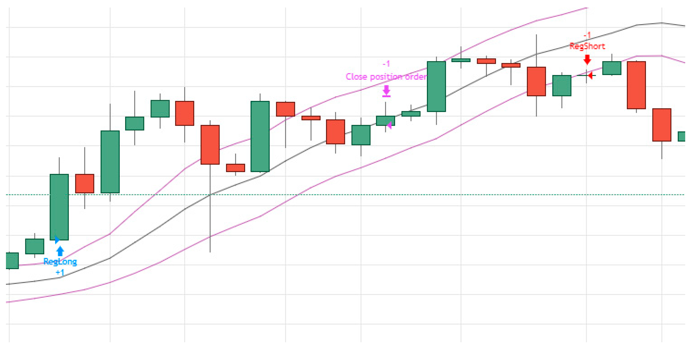
Figure 1 demonstrate how we used the linear regressions technique for algorithmic trading platforms.
A linear regression strategy demands the length of time for the line formation and the span from that line that determines the entry and exit from the trading positions. The regression line in Figure 1, for example, is based on 50 trading days when one standard deviation from that line determines the entry and exit points to the trading position. We started our PSO procedure with a random variable for both the daily time length and for the span that determined the actual entry and exits of trades. The system altered those variables in order to maximize our trading targets.
3.3. Darvas Boxes Strategy
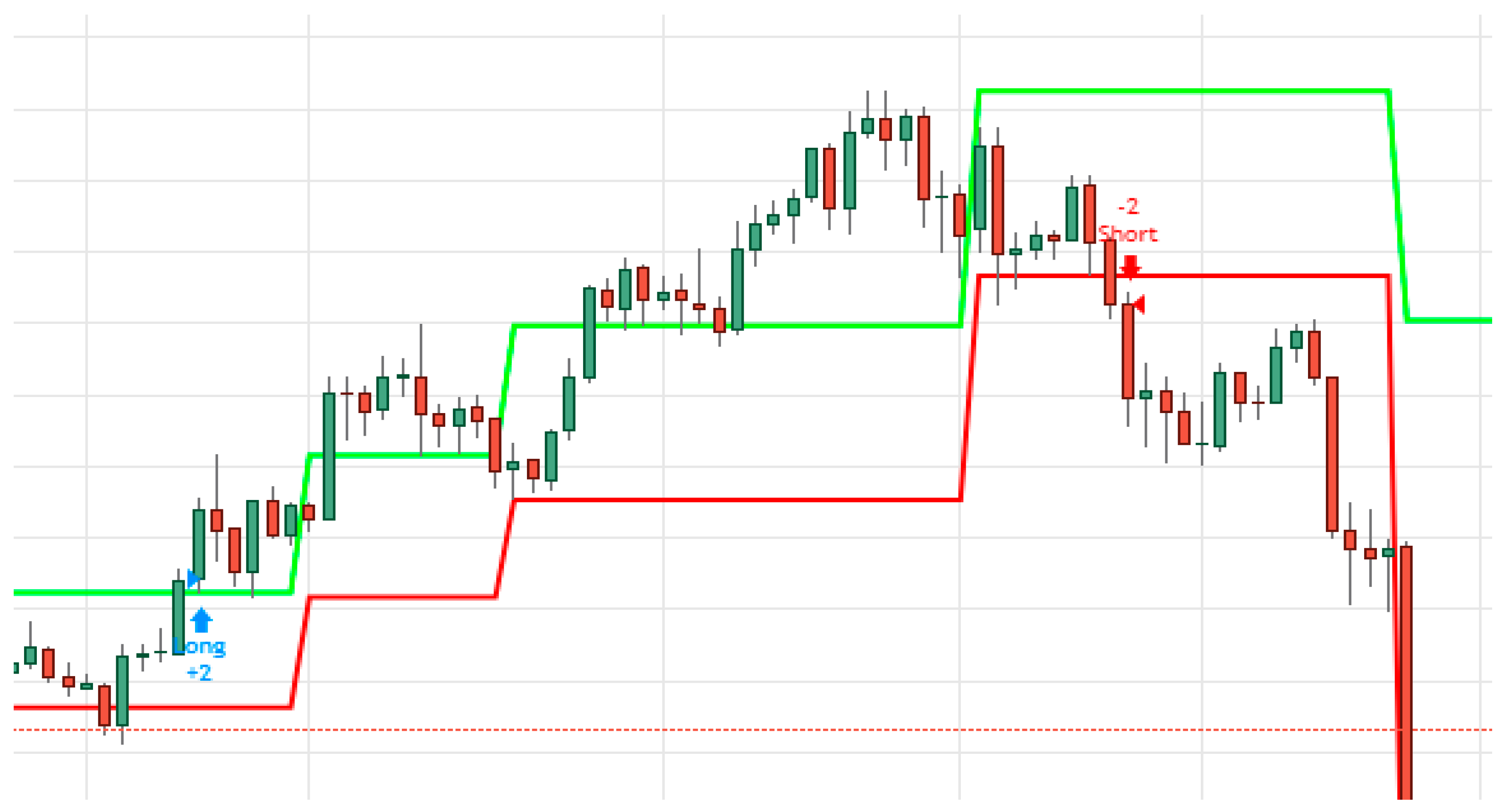
Figure 2 show an example of an automated trading platform using Darvas boxes.
Figure 2 show how Darvas boxes are designed and how they generate a long and short signal. This algorithmic trading system assumes that the trader is always exposed to price shifts between long and short positions. Darvas boxes use the notation that deviation from overtime horizontal support and resistance lines can be used to construct a winning trading strategy. The idea is that the asset’s price should move within a specific box formation when no external news is provided and break formation when important news concerning the commodity is introduced to the financial markets. Boxes can be formed using any predetermined time frame according to the financial asset’s volatility. A high volatility financial asset demands a shorter time frame for box formation than a low volatility asset. The PSO process starts with a random number of days to construct the boxes and alter them to achieve better trading performances. Once the size and shape of the boxes are formed in the training period, it is used for the tested period for which performances are remeasured.
3.4. Bollinger Bands Strategy
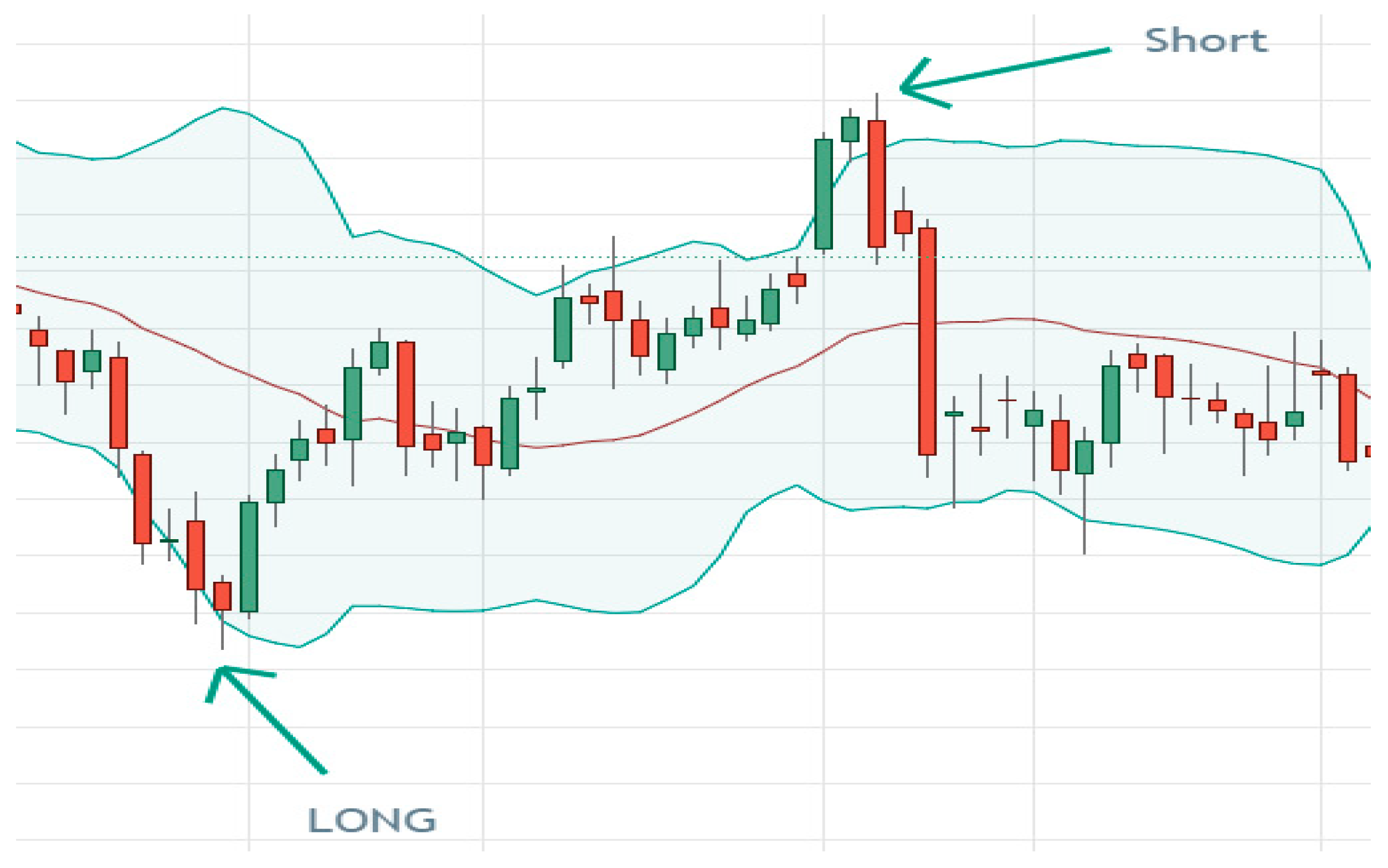
Bollinger bands (BB) (developed by John Bollinger) use two standard deviations away from a simple moving average. The trading strategy demonstrated in Figure 3 uses 14 days for the moving average calculation with the original two standard deviations. When the price of the commodity crosses the lower band, the system opens, a buy long order is placed, and when it crosses the upper band, a sell short order is generated.
The PSO procedures start with random setups for both the moving average and the standard deviations and optimize both particles of our trading system.
The three methodologies that were tested in this research are based on the pattern recognition of price movements of the precious metals. The LR tries to adjust a linear model (horizontal or diagonal) to the data and determine price direction through a deviation from that linear formation. The DB methodology works on a shorter-term formation of boxes that represent the horizontal support and resistance lines. A deviation from that formation can be used to identify price trends shifts and support trading decision making. The concept that lies behind the BB structure does not demand the identification of a predetermined formation but rather determines a zone in which the financial assets are expected to move within a specific time frame. A break-out of the price from the expected zone can indicate irregularities of movements and can be used to make profits.
4. Results
We start the results section by presenting 10 years of (until the end of April 2021) monthly and daily correlations matrix between the returns of the examined precious metals.
From Table 1, we learn that all examine precious metal monthly returns are positively correlated. However, on a daily level, the correlations between the precious metals prices do not have the same sign. While gold and silver and copper and silver are negatively correlated, platinum and palladium and silver and platinum are positively correlated. We now apply to the daily data our designated multi-dimension regression model (Equation (1)), and report the results for the standard stepwise regression model is presented in Table 2. This model enables us to better understand the one to three day lag dependencies of each metal to its previous price changes and to the other precious metals.
Table 2 show an interesting phenomenon, all precious metals’ current daily returns are negatively autocorrelated to their former days’ returns: gold and silver to their former three consecutive days returns, platinum to its two consecutive days returns, and copper and palladium to their single former day returns. In terms of interdependencies, Table 2 exhibit that gold current daily returns are negatively affected by silver’s former days’ returns. However, silver’s current daily returns are positively correlated to gold’s returns two and three days ago. Platinum’s current daily returns were found to be positively affected by gold, silver, and palladium’s past returns. Palladium’s current daily return was found to be positively correlated to yesterday’s returns of silver and platinum and two days ago of gold’s returns. The observations described above about the precious metals’ daily autocorrelations helped us better understand the fluency of daily prices to construct our trading strategy. All the designed trading systems are based on daily trading data. However, because of the different nature of these strategies, the number of days used for each of them which is determined solely by the optimization process, is different. For example, the linear regression system needs more days than the other methodologies to construct its formations; therefore, the algorithm needs a higher number of days to analyze the price trends and produce profitable trading signals than the systems that are based on Darvas boxes and Bollinger bands which are more dynamic in nature and demand fewer days to achieve their best performances.
4.1. Linear Regression Trading Strategy
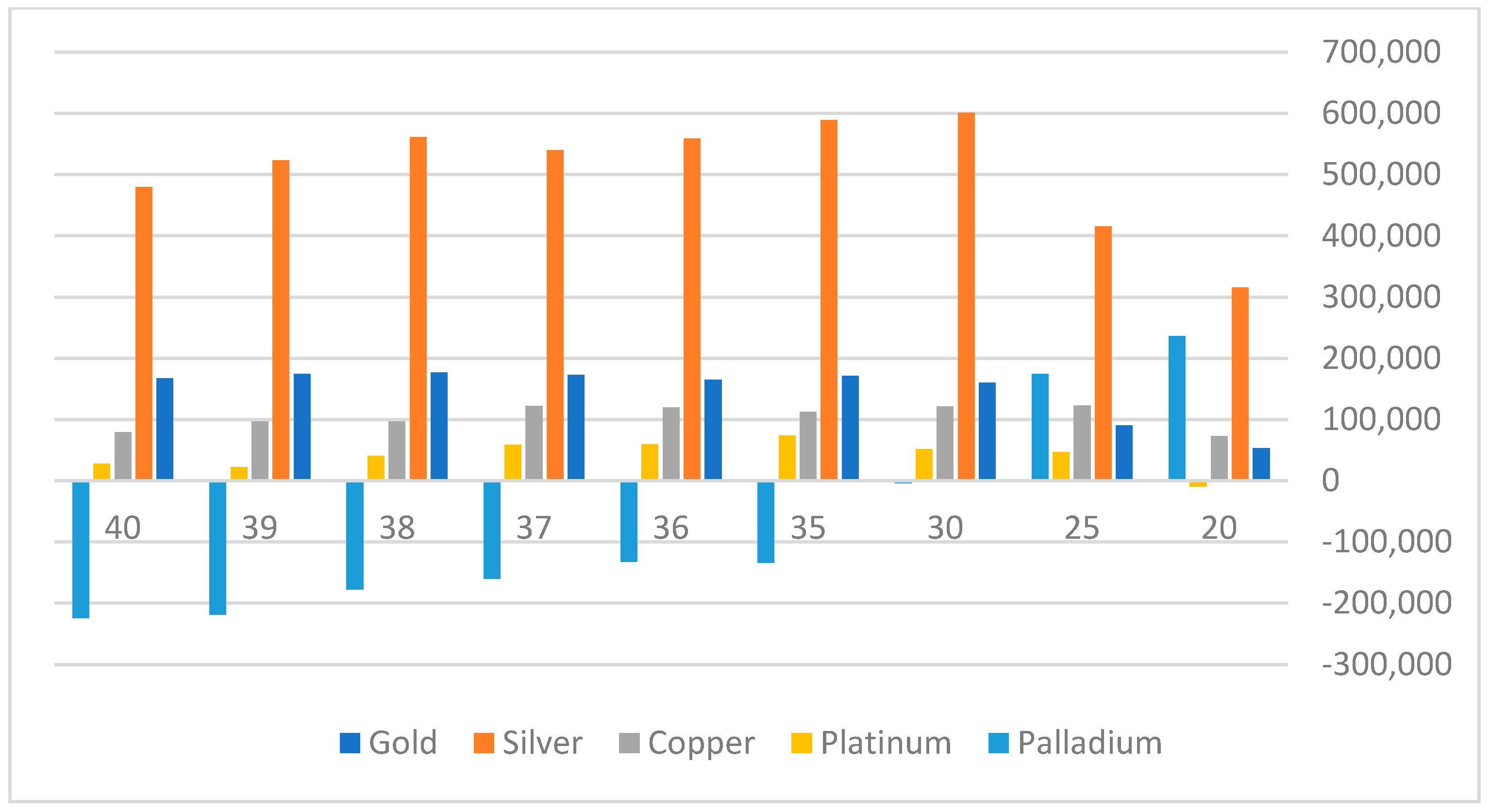
The linear regression strategy requires determining the number of days on which the linear regression line is formed. We start with a random number of days for each metal and optimize the trading results through our PSO system. The best trading results are summarized in Table 3 and Figure 4.
Table 3 and Figure 4 demonstrate that the linear regression methodology best fits to the trade of silver, palladium, and gold and fits less to the trade of copper and platinum. The best setup for gold and silver trading systems is 38 days, for which the system generated USD 177,198 and USD 561,425 NP, respectively. For palladium, the best setup is 20 days achieving an NP of USD 235,950 with a PF of 1.30. In Table 4, we split our trades into long and short trades to examine whether a difference in profitability will occur.
Table 4 indicate that the linear regression technique fits both long and short trades. However, it is a better strategy for long trades than for short trades for all the examined commodities. The difference in long and short trades is significant for all metals in terms of NP and PF. Silver, again, leads the other metals in both long and short trades, resulting in a PF of 1.8 for long trades and 1.55 for short trades.
4.2. Darvas Box Strategy
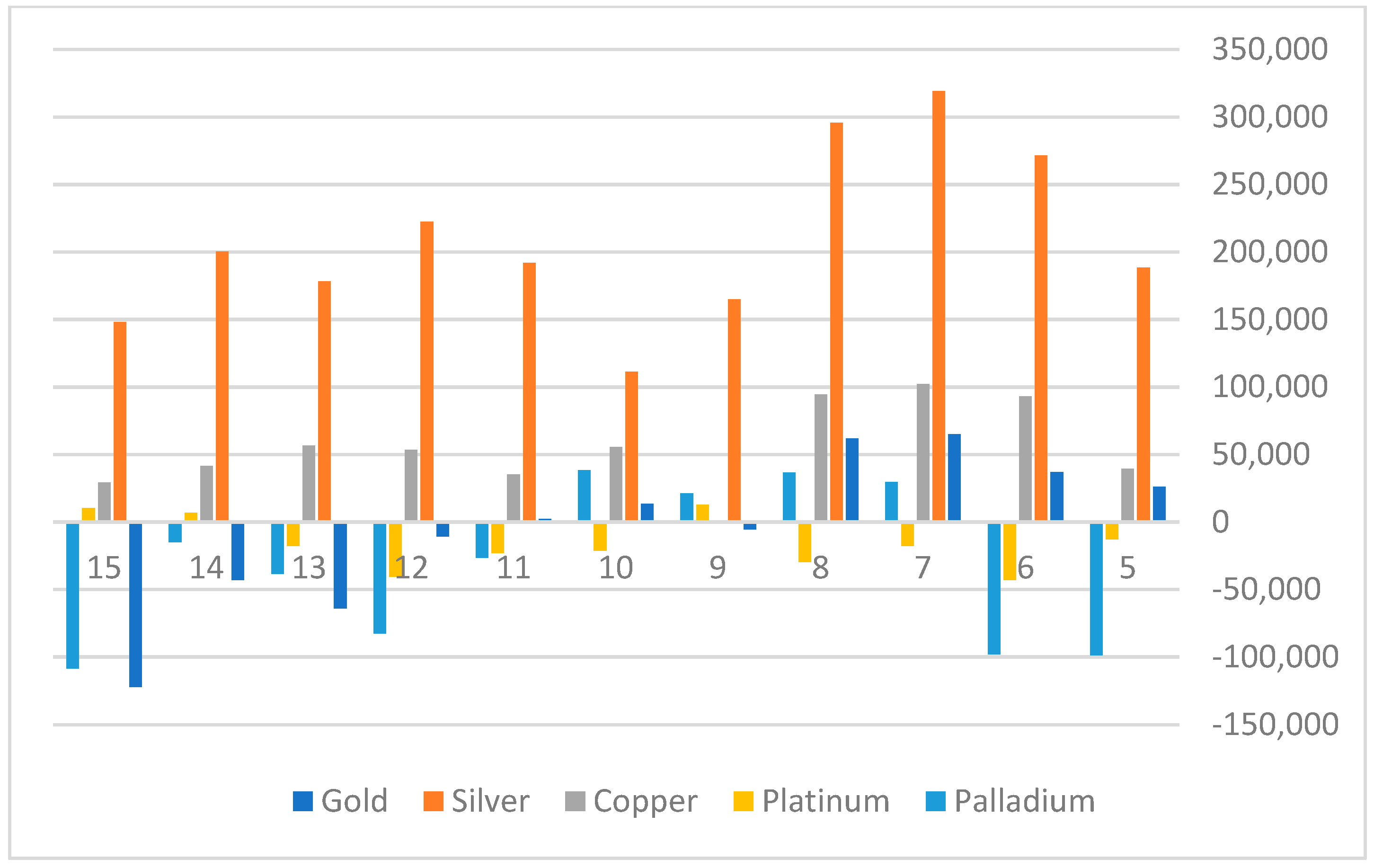
Darvas box strategy requires determining the number of days on which the system will build the boxes formations and deliver buy or sell signals. Again, we start with a random number of days and let our PSO system optimize our goal functions. The best trading results are summarized in Table 5 and Figure 5.
The trading results according to the Darvas boxes methodology described in Table 5 and Figure 5 show that this methodology, like the linear regression technique, best forecasts silver price trends than copper and gold, and it is less effective in forecasting future prices of platinum and palladium. Our system generated an NP of USD 319,200 for silver, with a PF of 1.55, using a 7-day setup. This setup was found to be useful also for gold and copper trading. Table 6 divide all the trades into long and short trades using the optimized setups for each metal.
The table shows that for all five precious metals, the system again performed better for long trades than for short trades. Moreover, short trades have produced losses for gold, platinum, and palladium. The only precious metals for which the Darvas boxes technique fits both long and short trade are silver and copper. These results indicate that the system based on the Darvas boxes methodology can better predict positive future price trends than negative trends.
4.3. Bollinger Band Strategy
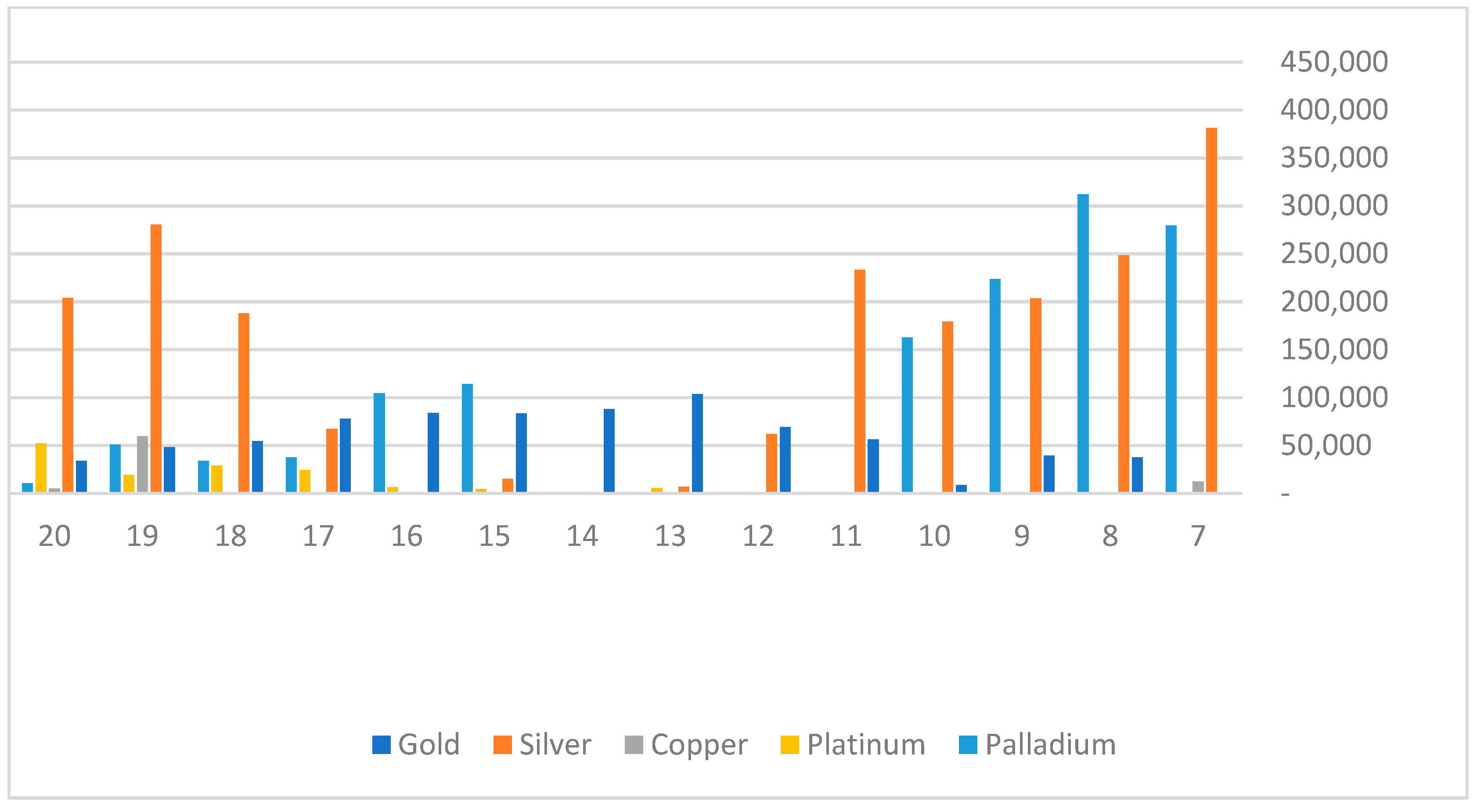
Table 7 summarize the results of the examined metals prices using the Bollinger band (BB) technique. This methodology calculates a moving average of a predetermined number of the trading day and contrasts the upper and lower bands using two standard deviations from that moving average. Using our PSO system, we optimized the trading results for each commodity in terms of NP, PP, and PF. The results are presented in Table 7 and Figure 6.
Table 7 and Figure 6 indicate that BB best forecasts silver and palladium futures prices, and it is less effective for copper and platinum. Seven days was found to be the best setup for silver and palladium, while 13 days best fit the gold price forecast. It is worth noting that silver and palladium prices are more volatile than the other metals, as was demonstrated in Table 1, resulting in relatively fewer preferred days setups for the BB methodology. The BB technique provided better percent of profitable (PP) results for all metals than the linear regression or the Darvas boxes techniques making it the lowest risk algorithmic trading system. Table 8 split the trades for long and short trades.
Table 8 indicate that, again, the BB methodology also fits long than short trades better. This technique fails to predict the negative price trends of gold.
5. Summary and Implications
In this research, we examined the short-term behavior of five major precious metals and tried to determine whether prices can be predicted and traded accordingly to algorithmic trading systems. By using a multidimensional regression model, we found that all precious metals’ current daily returns are negatively autocorrelated to their former days’ returns. Gold and silver are negatively correlated to the former three consecutive days’ returns, platinum to two former days returns, and copper and palladium to a single former days’ returns. The model also identified lagged interdependencies among the examined metals. These findings helped us to better understand the daily price fluctuation of each metal and to improve the trading systems. The trading systems used three forecasts’ methodologies: linear regression (LR), Darvas boxes (DB), and Bollinger bands (BB). Our data consisted of 20 years of daily price data concerning five precious metals futures: gold, silver, copper, platinum, and palladium. During that long time, the precious metals experienced high and low price volatility under different economic conditions. We used PSO as our primary optimization tool because of the complexity of our target function. For that optimization process, we split our data into two equal time periods, 10 years of training and optimization of our system and 10 years of testing and reporting results.
We found that it is possible to forecast the short-term price trends of all the examined precious metals. Moreover, we documented that our system better forecasts price-up trends than downtrends for all examined techniques and commodities. Our systems best predict silver future prices and forecasts platinum prices the worst. Linear regression was found to be the best forecasting technique for silver and gold price trends, while the Bollinger band technique best fits palladium. This research has proven that precious metals prices can be predicted using an algorithmic trading system and, therefore, can be used by researchers, traders, and hedgers.
Funding
This research was funded by Western Galilee Academic College.
Institutional Review Board Statement
Not applicable.
Informed Consent Statement
Not applicable.
Data Availability Statement
Not applicable.
Conflicts of Interest
The author declares no conflict of interest.
References
- Chebbi, T. The response of precious metal futures markets to unconventional monetary surprises in the presence of uncertainty. Int. J. Financ. Econ. 2020, 26, 1897–1916. [Google Scholar] [CrossRef]
- Cohen, G. Forecasting Bitcoin Trends Using Algorithmic Learning Systems. Entropy 2020, 22, 838. [Google Scholar] [CrossRef] [PubMed]
- Bishop, C.M. Pattern Recognition and Machine Learning; Springer: Cambridge, UK, 2006. [Google Scholar]
- Poggio, T.; Girosi, F. Networks for approximation and learning. Proc. IEEE 1990, 78, 1481–1497. [Google Scholar] [CrossRef] [Green Version]
- Martino, L.; Read, J. Joint introduction to Gaussian Processes and Relevance Vector Machines with Connections to Kalman filtering and other Kernel Smoothers. Inf. Fusion 2021, 74, 17–38. [Google Scholar] [CrossRef]
- Tipping, M.E. Sparse Bayesian Learning and the Relevance Vector Machine. J. Mach. Learn. Res. 2001, 1, 211–244. [Google Scholar]
- Candela, J.Q. Learning with Uncertainty—Gaussian Processes and Relevance Vector Machines; Technical University of Denmark: Copenhagen, Denmark, 2004; pp. 1–152. [Google Scholar]
- Zheng, Y. The linkage between aggregate investor sentiment and metal futures returns: A nonlinear approach. Q. Rev. Econ. Financ. 2015, 58, 128–142. [Google Scholar] [CrossRef]
- Qadan, M. Risk appetite and the prices of precious metals. Resour. Policy 2019, 62, 138–153. [Google Scholar] [CrossRef]
- Sensoy, A. Dynamic relationship between precious metals. Resour. Policy 2013, 38, 504–511. [Google Scholar] [CrossRef]
- Bosch, D.; Pradkhan, E. The impact of speculation on precious metals futures markets. Resour. Policy 2015, 44, 118–134. [Google Scholar] [CrossRef]
- Kang, S.H.; McIver, R.; Yoon, S.M. Dynamic spillover effects among crude oil, precious metal, and agricultural commodity futures markets. Energy Econ. 2017, 62, 19–32. [Google Scholar] [CrossRef]
- Shahzad, J.H.; Rehman, M.U.; Jammazi, R. Spillovers from oil to precious metals: Quantile approaches. Resour. Policy 2019, 61, 508–521. [Google Scholar] [CrossRef]
- Alameer, Z.; Elaziz, M.A.; Ewees, A.A.; Haiwang, Y.; Zhang, J. Forecasting Copper Prices Using Hybrid Adaptive Neuro-Fuzzy Inference System and Genetic Algorithms. Nat. Resour. Res. 2019, 28, 1385–1401. [Google Scholar] [CrossRef]
- Cortez, C.A.T.; Saydam, S.; Coulton, J.; Sammut, C. Alternative techniques for forecasting mineral commodity prices. Int. J. Min. Sci. Technol. 2018, 28, 309–322. [Google Scholar] [CrossRef]
- Kennedy, J.; Eberhart, R.C. Practical Swarm Optimization. In Proceedings of the International Conference on Neural Networks, Perth, Australia, 27 November–1 December 1995; pp. 1942–1948. [Google Scholar]
- Eberhart, R.C.; Simpson, P.K.; Dobbins, R.W. Computational Intelligence PC Tools; Academic Press Professional: Boston, MA, USA, 1996. [Google Scholar]
Figure 1.
Linear regression algorithmic trading strategy. Notes: Every candlestick in Figure 1 represent the high/low open/close of the commodity futures’ daily prices. The middle line in Figure 1 represent the linear regression line, while the other two lines represent one standard deviation from it.

Figure 2.
Darvas boxes algorithmic trading strategy. Notes: Every candlestick in Figure 2 represent the high/low open/close Bitcoin daily prices. A green daily candle means that the close price is above the opening price and a red candle means that the close price is lower than the opening price. The green and red lines indicate the upper and lower boundaries of Darvas’s boxes.

Figure 3.
Bollinger Bands algorithmic trading strategy. Notes: A green daily candle means that the close price is above the opening price and a red candle means that the close price is lower than the opening price.The middle brown line is a simple moving average and the blue lines are the upper and lower boundaries of the BB.

Figure 4.
Net profits trading results of linear regression strategy.

Figure 5.
Net profits trading results of Darvas boxes strategy.

Figure 6.
Net profits trading results of Bollinger bands strategy.


Table 1.
Correlations matrix of monthly and daily returns.
| Period | Gold | Silver | Copper | Platinum | Palladium | |
|---|---|---|---|---|---|---|
| Gold | M | 1 | 0.75 | 0.25 | 0.51 | 0.28 |
| Silver | M | 0.75 | 1 | 0.45 | 0.61 | 0.44 |
| Copper | M | 0.25 | 0.45 | 1 | 0.56 | 0.51 |
| Platinum | M | 0.51 | 0.61 | 0.56 | 1 | 0.55 |
| Palladium | M | 0.28 | 0.44 | 0.51 | 0.55 | 1 |
| Gold | D | 1 | −0.032 | 0.015 | −0.015 | −0.032 |
| Silver | D | −0.032 | 1 | −0.029 | 0.017 | 0.031 |
| Copper | D | 0.015 | −0.029 | 1 | 0.015 | −0.029 |
| Platinum | D | −0.015 | 0.017 | 0.015 | 1 | 0.030 |
| Palladium | D | −0.032 | 0.031 | −0.029 | 0.030 | 1 |
Table 2.
Results of the regression model.
| Gold | ||||||||||
| Coeff | −0.20 * | −0.17 * | −0.04 * | −0.02 * | −0.02 * | 0.02 | 0.04 | 0.03 | 0.04 | |
| T stat | −11.00 | −9.48 | −2.14 | −2.82 | −2.04 | 0.97 | 1.86 | 1.57 | 1.73 | F = 21.6 |
| Silver | ||||||||||
| Coeff | −0.04 | 0.09 * | 0.06 * | −0.48 * | −0.26 * | −0.14 * | 0.26 * | 0.06 | ||
| T stat | −1.18 | 2.44 | 1.82 | −25.3 | −12.36 | −7.33 | 5.93 | 1.62 | F = 83.9 | |
| Copper | ||||||||||
| Coeff | 0.01 | 0.01 | −0.01 | 0.01 | 0.01 | −0.02 | −0.05 * | 0.02 | ||
| T stat | 0.75 | 0.72 | 0.73 | 1.26 | 0.15 | −1.41 | −2.42 | 1.14 | F = 2.7 | |
| Platinum | ||||||||||
| Coeff | 0.03 * | 0.11 * | 0.09 * | 0.04 * | −0.02 | −0.07 * | −0.03 * | 0.09 * | 0.08 * | |
| T stat | 1.95 | 14.65 | 10.65 | 5.60 | 1.27 | −3.93 | −2.05 | 6.73 | 5.85 | F = 39.4 |
| Palladium | ||||||||||
| Coeff | 0.04 * | −0.02 | 0.04 * | 0.01 | 0.02 | 0.02 | −0.05 | 0.06 * | 0.08 * | |
| T stat | 2.17 | −1.04 | 3.78 | 1.39 | 1.75 | 0.76 | −1.85 | 2.26 | 4.33 | F = 16.64 |
Notes: daily returns of gold, silver, copper, platinum, and palladium, is 1…3 days ago daily returns of gold, silver, copper, platinum, and palladium. * = significant at 95% confidence level. = the proportion of the variation in the dependent variable that is predictable from the independent variable(s). F = Statistic test results that measure the fitness of the model to the data. T stat = the ratio of the departure of the estimated value of a parameter from its hypothesized value to its standard error.
Table 3.
Linear regression strategy trading results.
| Days | Gold | Silver | Copper | Platinum | Palladium | |
|---|---|---|---|---|---|---|
| 20 | NP | 53,390 | 315,150 | 72,612 | −9705 | 235,950 ** |
| PP | 45.48% | 44.54% | 43.88% | 42.92% | 40.67% | |
| PF | 1.06 | 1.25 | 1.14 | 0.98 | 1.30 | |
| 25 | NP | 90,680 | 415,175 | 122,662 ** | 46,715 | 174,050 |
| PP | 42.96% | 44.18% | 44.71% | 43.5% | 39.14% | |
| PF | 1.13 | 1.40 | 1.22 | 1.10 | 1.23 | |
| 30 | NP | 159,810 | 600,750 | 121,450 | 51,955 | −4300 |
| PP | 45.55% | 46.26% | 43.87% | 42.7% | 39.7% | |
| PF | 1.26 | 1.67 | 1.24 | 1.13 | 0.99 | |
| 35 | NP | 171,040 | 589,150 | 112,862 | 73,445 ** | −133,650 |
| PP | 43.89% | 44.4% | 44.41% | 43.92% | 8.8% | |
| PF | 1.31 | 1.71 | 1.26 | 1.18 | 0.83 | |
| 36 | NP | 165,180 | 558,975 | 119,837 | 59,225 | −132,400 |
| PP | 42.6% | 43.91% | 44.48% | 43.25% | 37.78% | |
| PF | 1.30 | 1.64 | 1.28 | 1.15 | 0.83 | |
| 37 | NP | 172,600 | 539,700 | 122,187 | 59,005 | −159,950 |
| PP | 42.63% | 45.1% | 44.65% | 42.53% | 37.76% | |
| PF | 1.30 | 1.65 | 1.29 | 1.15 | 0.80 | |
| 38 | NP | 177,190 ** | 561,425 ** | 96,737 | 40,110 | −177,300 |
| PP | 42.48% | 44.15% | 42.46% | 41.72% | 38.04% | |
| PF | 1.32 | 1.69 | 1.22 | 1.09 | 0.78 | |
| 39 | NP | 174,600 | 523,050 | 96,787 | 22,160 | −219,000 |
| PP | 43.78% | 43.46% | 41.62% | 39.93% | 37.09% | |
| PF | 1.32 | 1.63 | 1.22 | 1.05 | 0.73 | |
| 40 | NP | 167,460 | 480,000 | 79,400 | 27,700 | −224,150 |
| PP | 43% | 41.64% | 42.5% | 40.14% | 36.55% | |
| PF | 1.31 | 1.58 | 1.18 | 1.069 | 0.73 |
Notes: NP = Net profit, PP = Percent of profitable trades of all trades, PF = Profit factor, Days= The number of days on which the linear regression is constructed. ** = The highest NP.
Table 4.
Linear regression trading results of long/short strategies.
| Days | Gold | Silver | Copper | Platinum | Palladium | |
|---|---|---|---|---|---|---|
| Long | NP | 163,650 | 341,900 | 79,500 | 54,460 | 213,600 |
| PP | 44.4% | 45.6% | 49.3% | 46.5% | 44.3% | |
| PF | 1.6 | 1.82 | 1.39 | 1.3 | 1.67 | |
| Short | NP | 13,540 | 219,525 | 42,687 | 18,985 | 22,350 |
| PP | 41% | 42.5% | 39.8% | 41.3% | 37.3% | |
| PF | 1.05 | 1.55 | 1.2 | 1.09 | 1.05 |
Notes: NP = Net profit, PP = Percent of profitable trades of all trades, PF = Profit factor. The results for gold and silver are calculated according to their optimum setups of 38 days, copper 37 days, platinum 35 days, and palladium 20 days.
Table 5.
Darvas boxes strategy trading results.
| Days | Gold | Silver | Copper | Platinum | Palladium | |
|---|---|---|---|---|---|---|
| 5 | NP | 26,080 | 188,475 | 39,487 | −12,725 | −98,550 |
| PP | 37.30% | 36% | 35.45% | 37.8% | 34.12% | |
| PF | 1.05 | 1.22 | 1.09 | 0.97 | 0.86 | |
| 6 | NP | 36,990 | 271,625 | 93,087 | −42,775 | −97,950 |
| PP | 36.67% | 36.24% | 36% | 37.9% | 33% | |
| PF | 1.08 | 1.36 | 1.26 | 0.88 | 0.85 | |
| 7 | NP | 65,290 ** | 319,200 ** | 102,175 ** | −17,735 | 29,550 |
| PP | 39.54% | 37.75% | 35.19% | 36.36% | 33.06% | |
| PF | 1.17 | 1.55 | 1.31 | 0.95 | 1.06 | |
| 8 | NP | 61,830 | 295,650 | 94,425 | −29,445 | 36,750 |
| PP | 38.49% | 37.54% | 37.81% | 37.13% | 33.18% | |
| PF | 1.17 | 1.55 | 1.31 | 0.91 | 1.07 | |
| 9 | NP | −5290 | 164,800 | 94,925 | 13,035 ** | 21,150 |
| PP | 36.33% | 35.07% | 40.11% | 37% | 33.51% | |
| PF | 0.98 | 1.28 | 1.35 | 1.05 | 1.04 | |
| 10 | NP | 13,610 | 111,125 | 55,662 | −21,020 | 38,650 ** |
| PP | 33.62% | 33.59% | 38.79% | 32.32% | 33.14% | |
| PF | 1.04 | 1.19 | 1.20 | 0.93 | 1.09 | |
| 11 | NP | 2500 | 191,875 | 35,412 | −22,795 | −26,250 |
| PP | 35.61% | 34.05% | 39.1% | 29.94% | 32.7% | |
| PF | 1.00 | 1.38 | 1.13 | 0.92 | 0.94 | |
| 12 | NP | −10,760 | 222,425 | 53,537 | −40,555 | −82,450 |
| PP | 35.68% | 36.89% | 39.86% | 29.7% | 31.37% | |
| PF | 0.97 | 1.52 | 1.21 | 0.85 | 0.83 | |
| 13 | NP | −63,780 | 178,125 | 56,737 | −17,490 | −38,350 |
| PP | 30.415 | 34 % | 39% | 30.61% | 34% | |
| PF | 0.83 | 1.39 | 1.24 | 0.93 | 0.91 | |
| 14 | NP | −43,000 | 200,275 | 41,762 | 6990 | −14,950 |
| PP | 32.15 | 35.71% | 37.3% | 32.33% | 36.22% | |
| PF | 0.87 | 1.47 | 1.18 | 1.03 | 0.96 | |
| 15 | NP | −122,000 | 148,125 | 29,212 | 10,590 | −108,550 |
| PP | 34% | 32.56% | 35.45% | 31.93% | 33.88% | |
| PF | 0.96 | 1.32 | 1.13 | 1.05 | 0.75 |
Notes: NP = Net profit, PP = Percent of profitable trades of all trades, PF = Profit factor, Days = The number of days on which the Darvas box is constructed. ** = The highest NP.
Table 6.
Darvas boxes trading results of long/short strategies.
| Days | Gold | Silver | Copper | Platinum | Palladium | |
|---|---|---|---|---|---|---|
| Long | NP | 111,170 | 222,425 | 95,863 | 28,335 | 152,550 |
| PP | 41.815 | 39.55% | 39.32% | 42.155 | 39.77% | |
| PF | 1.77 | 1.93 | 1.79 | 1.28 | 2.02 | |
| Short | NP | −45,880 | 96,775 | 6312 | −15,300 | −113,900 |
| PP | 37.25% | 35.96% | 31.03% | 31.7% | 26.44% | |
| PF | 0.81 | 1.28 | 1.03 | 0.91 | 0.58 |
Notes: NP = Net profit, PP = Percent of profitable trades of all trades, PF = Profit factor. The results for gold, silver, and copper are calculated according to their optimum setups of 7 days, platinum 9 days, and palladium 10 days.
Table 7.
Bollinger bands strategy trading results.
| Days | Gold | Silver | Copper | Platinum | Palladium | |
|---|---|---|---|---|---|---|
| 7 | NP | −60 | 381,325 ** | 12,462 | −8450 | 279,350 |
| PP | 60.2% | 62.5% | 64.7% | 61.1% | 56.1% | |
| PF | 1.0 | 1.67 | 1.03 | 0.97 | 1.80 | |
| 8 | NP | 37,470 | 248,425 | −84,162 | −80,850 | 311,950 ** |
| PP | 59.8% | 61% | 63.6% | 63.3% | 61% | |
| PF | 1.08 | 1.34 | 0.82 | 0.77 | 1.70 | |
| 9 | NP | 39,690 | 203,425 | −89,450 | −88,335 | 223,700 |
| PP | 59.2% | 63% | 62.5% | 65% | 58.4% | |
| PF | 1.08 | 1.27 | 0.81 | 0.75 | 1.43 | |
| 10 | NP | 8730 | 179,175 | −90,262 | −72,165 | 162,600 |
| PP | 58.2% | 65.5% | 63.1% | 65% | 60% | |
| PF | 1.02 | 1.26 | 0.80 | 0.80 | 1.30 | |
| 11 | NP | 56,330 | 233,175 | −64,937 | −28,080 | −118,800 |
| PP | 60.6% | 65.9% | 62.4% | 65.5% | 57.9% | |
| PF | 1.13 | 1.35 | 0.85 | 0.92 | 0.80 | |
| 12 | NP | 69,310 | 61,925 | −84,000 | −31,120 | −87,400 |
| PP | 63.8% | 65.9% | 65.1% | 66.5% | 59.2% | |
| PF | 1.16 | 1.09 | 0.81 | 0.90 | 0.85 | |
| 13 | NP | 103,760 ** | 7100 | −63,812 | 5690 | −116,000 |
| PP | 63.7% | 63.5% | 65.6% | 64.5% | 58.7% | |
| PF | 1.25 | 1.01 | 0.85 | 1.02 | 0.79 | |
| 14 | NP | 88,190 | −21,100 | −68,412 | −6050 | −22,100 |
| PP | 63.6% | 62.8% | 64.3% | 63.1% | 59.6% | |
| PF | 1.22 | 0.97 | 0.83 | 0.98 | 0.96 | |
| 15 | NP | 83,580 | 14,950 | −67,437 | 4660 | 114,150 |
| PP | 62.6% | 64.3% | 64.5% | 65.6% | 61.3% | |
| PF | 1.21 | 1.02 | 0.83 | 1.02 | 1.25 | |
| 16 | NP | 83,890 | 700 | −4562 | 6300 | 104,650 |
| PP | 63% | 65.5% | 66.7% | 66.3% | 60.8% | |
| PF | 1.21 | 1.0 | 0.98 | 1.02 | 1.24 | |
| 17 | NP | 77,980 | 67,225 | −46,887 | 24,120 | 37,750 |
| PP | 62.5% | 66.1% | 61.9% | 66% | 60.3% | |
| PF | 1.2 | 1.1 | 0.87 | 1.09 | 1.08 | |
| 18 | NP | 54,520 | 187,975 | −13,837 | 28,780 | 33,950 |
| PP | 62.3% | 67.4% | 63.8% | 67.8% | 62.3% | |
| PF | 1.14 | 1.33 | 0.96 | 1.11 | 1.07 | |
| 19 | NP | 48,340 | 280,495 | 59,812 ** | 19,250 | 50,950 |
| PP | 63.6% | 67.5% | 65.7% | 68.8% | 63% | |
| PF | 1.13 | 1.54 | 1.18 | 1.07 | 1.10 | |
| 20 | NP | 33,920 | 203,975 | 5262 | 52,500 ** | 10,550 |
| PP | 61.2% | 66.8% | 65.8% | 69.8% | 62.9% | |
| PF | 1.09 | 1.41 | 1.02 | 1.19 | 1.02 |
Notes: NP = Net profit, PP = Percent of profitable trades of all trades, PF = Profit factor, Days = The number of days on which the Bollinger band is constructed. ** = The highest.
Table 8.
Bollinger bands trading results of long/short strategies.
| Days | Gold | Silver | Copper | Platinum | Palladium | |
|---|---|---|---|---|---|---|
| Long | NP | 134,490 | 252,425 | 57,137 | 48,370 | 262,800 |
| PP | 65.7% | 63.5% | 64.7% | 73.2% | 64.7% | |
| PF | 1.85 | 2.12 | 1.37 | 1.35 | 2.65 | |
| Short | NP | −30,730 | 128,900 | 2675 | 4130 | 49,150 |
| PP | 61.7% | 61.5% | 66.7% | 66.4% | 57.5% | |
| PF | 0.88 | 1.37 | 1.02 | 1.03 | 1.17 |
Notes: NP = Net profit, PP = Percent of profitable trades of all trades, PF = Profit factor. The results for gold, silver, and copper are calculated according to their optimum setups of 7 days, platinum 9 days, and palladium 10 days.
Publisher’s Note: MDPI stays neutral with regard to jurisdictional claims in published maps and institutional affiliations. |
© 2022 by the author. Licensee MDPI, Basel, Switzerland. This article is an open access article distributed under the terms and conditions of the Creative Commons Attribution (CC BY) license (https://creativecommons.org/licenses/by/4.0/).
Share and Cite
MDPI and ACS Style
Cohen, G. Algorithmic Strategies for Precious Metals Price Forecasting. Mathematics 2022, 10, 1134. https://doi.org/10.3390/math10071134
AMA Style
Cohen G. Algorithmic Strategies for Precious Metals Price Forecasting. Mathematics. 2022; 10(7):1134. https://doi.org/10.3390/math10071134
Chicago/Turabian StyleCohen, Gil. 2022. "Algorithmic Strategies for Precious Metals Price Forecasting" Mathematics 10, no. 7: 1134. https://doi.org/10.3390/math10071134
Note that from the first issue of 2016, this journal uses article numbers instead of page numbers. See further details here.