Article

Testing for the Rayleigh Distribution: A New Test with Comparisons to Tests for Exponentiality Based on Transformed Data

by
Gerrit Lodewicus Grobler
,
Elzanie Bothma
* and
James Samuel Allison
School of Mathematical and Statistical Sciences, Faculty of Natural and Agricultural Sciences, North-West University, Potchefstroom 2531, South Africa
*
Author to whom correspondence should be addressed.
Mathematics 2022, 10(8), 1316; https://doi.org/10.3390/math10081316
Submission received: 15 March 2022 / Revised: 5 April 2022 / Accepted: 7 April 2022 / Published: 15 April 2022
(This article belongs to the Special Issue Probability, Stochastic Processes and Optimization)

Abstract

:
We propose a new goodness-of-fit test for the Rayleigh distribution which is based on a distributional fixed-point property of the Stein characterization. The limiting null distribution of the test is derived and the consistency against fixed alternatives is also shown. The results of a finite-sample comparison is presented, where we compare the power performance of the new test to a variety of other tests. In addition to existing tests for the Rayleigh distribution we also exploit the link between the exponential and Rayleigh distributions. This allows us to include some powerful tests developed specifically for the exponential distribution in the comparison. It is found that the new test outperforms competing tests for many of the alternative distributions. Interestingly, the highest estimated power, against all alternative distributions considered, is obtained by one of the tests specifically developed for the Rayleigh distribution and not by any of the exponentiality tests based on the transformed data. The use of the new test is illustrated on a real-world COVID-19 data set.

1. Introduction

In 1880 an acoustics problem gave rise to a distribution that nowadays plays a prominent role in research fields such as reliability theory, life testing and survival analysis (see, e.g., [1]). The Rayleigh distribution was introduced by [2], while undertaking a study regarding the resultant of a great number of sound waves with differing phases. Refs. [3,4] demonstrated the importance of the Rayleigh distribution in communication engineering and electro-vacuum devices, respectively. Ref. [5] found that the Rayleigh distribution has clinical applications, specifically estimating the noise variance of Magnetic Resonance Images (MRI). Ref. [6] discusses this phenomenon and proposed that this estimation can be done by fitting the density function of the Rayleigh distribution to the partial histogram of the MRI. Ref. [7] improved this estimation with the use of background segmentation, by fitting the density function of the Rayleigh distribution to the histogram of the segmented background in order to estimate the noise variance. The estimation of the noise forms a crucial part in efficiently denoising the MRI as well as in the quality assessment of these images. The Rayleigh distribution has also become a popular model in survival analysis and reliability theory, see, e.g., [8,9].
For any of the above-mentioned applications to be relevant, it is crucial to test the hypothesis that the observed data are indeed realisations from a Rayleigh distribution. Since the square of a Rayleigh distributed variable is exponentially distributed, goodness-of-fit tests designed for the exponential distribution can be used to test for the Rayleigh distribution—a fact that we investigate further in Section 4. However, even though the applications of the Rayleigh distribution increased significantly over the past few decades, literature on tests specifically developed for the Rayleigh distribution is relatively scarce. Some of these include a test proposed by [10] based on the empirical Laplace transform, a test based on entropy suggested by [11] as well as [12] and an empirical likelihood based test by [13]. It has become a common approach to use distributional characterizations to propose goodness-of-fit testing procedures, see, e.g., Ref. [14] and the references therein. In this paper, we propose a new test for the Rayleigh distribution based on a modification of Stein’s characterization discussed by [15].
The standard Stein characterization (see [16]) of the normal distribution states that Z is standard normal if, and only if,
E [ g ( Z ) Z g ( Z ) ] = 0
is true for all absolute continuous functions g for which the expectation exists. Some applications, such as goodness-of-fit tests based on (1), are rather complicated, since the results depend on the choice of g. Instead of using this relationship, Ref. [17] characterised the standard normal distribution based on the zero bias distribution. A real valued random variable X * is said to have a X zero-bias distribution if
E [ g ( X * ) ] = E [ X g ( X ) ]
holds for all absolutely continuous functions g for which the expectation exists. If E X = 0 and Var ( X ) = 1 , the X zero-bias distribution exists, is unique and has distribution function
F ( t ) = E [ X ( X t ) 1 { X t } ] , t R .
Using this distribution function, ref. [17] showed that Z is standard normal if, and only if, the distribution function of Z is given by F ( t ) . Ref. [15] generalised this method to a wide range of continuous distributions by generalising Stein’s characterization. They showed that if X has support [ 0 , ) , then it has distribution F if, and only if, the distribution function of X is given by
F ( t ) = E f ( X ) f ( X ) min { X , t } , t ( 0 , ) ,
where f is the density of X. The result in (2) is true under some regularity conditions on f, which will be discussed in Section 2. The characterization in (2) will be used to develop a new goodness-of-fit test specifically for the Rayleigh distribution.
Before proceeding some notation is introduced. Let X 1 , , X n be independent and identically distributed (i.i.d.) continuous realisations of a positive random variable X with unknown distribution function F and density f. If X follows a Rayleigh distribution with density function
f ( x ) = x θ 2 e x 2 2 θ 2 , x 0 , θ > 0 ,
it will be denoted by X R a l ( θ ) . The composite goodness-of-fit hypothesis to be tested is
H 0 :   the   distribution   of   X   is   R a l ( θ ) ,
for some θ > 0 , against general alternatives.
The remainder of the article is organised as follows: In Section 2, the new test statistic is introduced. Section 3 contains the basic theoretical results pertaining to the asymptotic behaviour of the test. The results of a Monte Carlo study, where the power performance of the newly proposed test is compared to some existing tests, is given in Section 4. The competing tests also include five powerful tests for exponentiality based on transformed data. The paper concludes in Section 5 with an application of the test to a real-world COVID-19 data set and some concluding remarks.

2. Test Statistic

For the characterization in (2) to be true the following regularity conditions, see [15], should hold:
(I)
f is continuously differentiable on [ 0 , ) ;
(II)
f ( x ) > 0 for every x [ 0 , ) ;
(III)
for κ f ( x ) = f ( x ) min { F ( x ) , 1 F ( x ) } f 2 ( x ) we have sup x [ 0 , ] κ f ( x ) < ;
(IV)
0 ( 1 + | x | ) | f ( x ) | d x < ;
(V)
lim x 0 F ( x ) f ( x ) = 0 ;
(VI)
lim x 1 F ( x ) f ( x ) = 0 .
It can easily be seen that conditions (I), (II), (V) and (VI) hold for the Rayleigh distribution. For X R a l ( θ ) , κ f in condition (III) becomes
κ f ( x ) = θ 2 e x 2 / 2 θ 2 x 2 min { F ( x ) , 1 F ( x ) } 1 x 2 θ 2
and for x 2 > θ 2 ; 1 x 2 θ 2 = x 2 θ 2 1 . For x large enough we have that 1 F ( x ) < F ( x ) ; thus,
lim x κ f ( x ) = θ 2 lim x exp ( x 2 / 2 θ 2 ) x 2 ( 1 F ( x ) ) x 2 θ 2 1 = 1
Because x is sufficiently small, we have that F ( x ) < 1 F ( x ) ; thus, we have
lim x 0 κ f ( x ) = θ 2 lim x 0 exp ( x 2 / 2 θ 2 ) 1 x 2 θ 2 1 e x 2 / 2 θ 2 x 2 = 1 2 θ 2 θ 2 = 1 2 .
Since κ f ( x ) is continuous with limits 1 and 1 2 as x tends to infinity and zero, respectively, it implies that sup x [ 0 , ) κ f ( x ) < .
The integral in condition (IV) can be written as follows in terms of expectations:
0 ( 1 + | x | ) 1 x 2 θ 2 1 θ 2 e x 2 / 2 θ 2 d x = E { 1 + X } 1 X 2 θ 2 ,
where X is Rayleigh distributed. The finite moments of the Rayleigh distribution exist, i.e., E ( X k ) < , k N . Therefore,
0 ( 1 + | x | ) | f ( x ) | d x < .
In Proposition 1 below, the characterization in (2) is re-stated specifically for the Rayleigh distribution.
Proposition 1.
Let X : Ω ( 0 , ) be a random variable with distribution function F and density function f that satisfies conditions (I)–(VI) and E [ X ] < . Then X R a l ( θ ) if, and only if,
E X θ 2 1 X min { X , t } F ( t ) = 0 , t > 0 .
Note that X R a l ( θ ) if, and only if, Y = X θ R a l ( 1 ) . This follows from the invariance property of the Rayleigh distribution with respect to scale transformations. This implies that Y R a l ( 1 ) if, and only if, for all t > 0
ψ ( t ) = T Y ( t ) F Y ( t ) = 0 ,
where T Y ( t ) = E Y 1 / Y min ( Y , t ) and F Y is the distribution function of Y. Our newly proposed test is motivated by (4). Since ψ ( t ) will be unknown, we estimate it by its empirical counterpart,
ψ ^ n ( t ) = T n Y ( t ) F n Y ( t ) ,
where T n Y ( t ) = 1 n j = 1 n Y j 1 / Y j min ( Y j , t ) , F n Y ( t ) = 1 n j = 1 n I ( Y j t ) and Y j = X j / θ ^ n , with θ ^ n = ( 2 n ) 1 j = 1 n X j 2 the maximum likelihood estimator for θ .
We propose the following weighted L 2 distance between ψ ^ ( t ) and 0 to test the hypothesis in (3):
R n , a = n 0 ψ ^ n 2 ( t ) w a ( t ) d t ,
where w a ( t ) is a positive, continuous weight function depending on a positive tuning parameter a. The test rejects for large values of R n , a . Throughout the paper we use w a ( t ) = e a t as the weight function, which results in the following easily calculable form of the test statistic:
R n , a = 1 n j = 1 n 1 a e a Y ( j ) Y ( j ) 1 Y ( j ) 2 2 a Y ( j ) + 2 a 2 + 2 Y ( j ) 2 3 + 2 a 3 Y ( j ) 2 2 + 1 Y ( j ) 2 + 2 n 1 j < k n Y ( j ) 1 Y ( j ) Y ( k ) 1 Y ( k ) 1 a e a Y ( j ) 1 a Y ( j ) + 2 a 2 + 2 a 3 Y ( j ) a 2 e a Y ( k ) + Y ( j ) 1 Y ( j ) Y ( j ) a e a Y ( k ) + Y ( k ) 1 Y ( k ) 1 a 2 e a Y ( k ) 1 a e a Y ( j ) Y ( j ) + 1 a + 1 a e a Y ( k ) ,
where Y ( 1 ) < Y ( 2 ) < < Y ( n ) denotes the order statistics of Y 1 , , Y n .
Remark 1.
The most commonly used choices for the weight function w a ( · ) are w a ( t ) = e a | t | and w a ( t ) = e a t 2 (see, e.g., [18,19]). Due to the positive support of the Rayleigh distribution, we use w a ( t ) = e a | t | = e a t , t 0 . This choice does not only provide a close form expression for the test statistic, but also competitive powers which are reported in the Monte Carlo simulation study (see Section 4).

3. Asymptotics

In this section, we will first show that, under the null hypothesis, R n , a converges in distribution to a norm of a Gaussian element of the Hilbert space H = L 2 ( 0 , ) , B of measurable, square integrable functions. The norm | | · | | H that will be used is defined in terms of a random element G n of H , n N , by
| | G n | | H = 0 G n ( t ) 2 e a t d t 1 2 .
We will also show that the newly proposed test is consistent.
First note that by substituting t with s θ ^ n and Y j with X j θ ^ n in (5) the test statistic R n , a can be rewritten as
R n , a = 1 θ ^ n 0 n T ^ n X ( s ) F n X ( s ) 2 e a s / θ ^ n d s ,
where
T ^ n X ( s ) = 1 n θ ^ n 2 j = 1 n X j θ ^ n 2 X j min X j , s
is a continuous function.
To obtain our two main results, we use the following Lemma, in which the notation G n H n is used when | | G n H n | | H 2 = o P ( 1 ) , where o P ( 1 ) denotes a sequence of random variables that converge to zero in probability. We also assume, w.l.o.g., that θ = 1 .
Lemma 1.
Suppose X , X 1 , X 2 , are i.i.d. random variables with distribution function F X and E X 4 < . Let T ^ n X ( s ) be defined as in (7), then
T ^ n X ( s ) = 1 θ ^ n 2 T n X ( s ) + 1 θ ^ n 2 r n X ( s ) ,
where
r n X ( s ) = 1 n j = 1 n 1 X j min X j , s ,
and
T n X ( s ) = 1 n j = 1 n X j 1 X j min ( X j , s ) .
We also have that
n T ^ n X ( s ) n θ ^ n 2 T n X ( s ) + 1 θ ^ n 2 r X ( s ) ,
where
r X ( s ) = E 1 X min X , s .
Proof. 
The first result follows immediately by rewriting T ^ n X ( s ) in (7) as
T ^ n X ( s ) = 1 n θ ^ n 2 j = 1 n X j 1 X j min X j , s + 1 X j θ ^ n 2 X j min X j , s .
To show the second result we notice that
n T ^ n X ( s ) 1 θ ^ n 2 T n X ( s ) + 1 θ ^ n 2 r X ( s ) = n 1 θ ^ n 2 θ ^ n 2 r n X ( s ) r X ( s ) .
Applying a weak form of the law of large numbers in separable Hilbert spaces, we have that r n X ( s ) = r X ( s ) + o P ( 1 ) and by the continuous mapping theorem | | r X r n X | | H 2 = o P ( 1 ) . Since θ ^ n 2 is the maximum likelihood estimator of θ 2 , we have that n 1 θ ^ n 2 = O P ( 1 ) , where O P ( 1 ) denotes a sequence of random variables that is bounded in probability. The result then follows from Slutsky’s theorem. □
Theorem 1.
Let X , X 1 , X 2 , be i.i.d. standard Rayleigh random variables. There exists a centred Gaussian element W of H such that R n , a D | | W | | H 2 , where the covariance kernel of W is given by
K ( s , t ) = Cov W j ( s ) , W j ( t ) = F X ( s t ) + s t I 3 ( s t , s t ) 2 I 1 ( s t , s t ) + I 1 ( s t , s t ) + s t 2 F X ( s t ) 2 + I 2 ( s t , ) + I 2 ( s t , ) + I 4 ( 0 , s t ) 2 I 2 ( 0 , s t ) + r X ( s ) r X ( t ) + 2 F X ( s ) F X ( t ) + 1 2 I 4 ( 0 , s ) + 3 2 I 2 ( 0 , s ) + s 1 2 I 3 ( s , ) + 3 2 I 1 ( s , ) + I 1 ( s , ) r X ( t ) + 1 2 I 4 ( 0 , t ) + 3 2 I 2 ( 0 , t ) + t 1 2 I 3 ( t , ) + 3 2 I 1 ( t , ) + I 1 ( t , ) r X ( s ) 1 2 I 4 ( 0 , s ) I 2 ( 0 , s ) + s I 3 ( s , ) + I 1 ( s , ) F X ( t ) 1 2 I 4 ( 0 , t ) I 2 ( 0 , t ) + t I 3 ( t , ) + I 1 ( t , ) F X ( s ) ,
where
I k ( a , b ) = E X j k 1 a X j b
and
I k ( a , ) = lim b I k ( a , b ) .
Proof. 
First note that
n T ^ n X ( s ) F n X ( s ) n θ ^ n 2 T n X ( s ) + 1 θ ^ n 2 r X ( s ) θ ^ n 2 F X ( s ) ,
since | | F X F n X | | H 2 = o P ( 1 ) . We can therefore write
n T ^ n X ( s ) F n X ( s ) 1 n θ ^ n 2 j = 1 n W j ( s ) ,
where
W j ( s ) = X j 1 X j min X j , s + 1 1 2 X j 2 r X ( s ) 1 2 X j 2 F X ( s ) .
We note that W 1 , , W n are i.i.d. random variables with E ( W 1 ) = 0 and E | | W 1 | | H 2 < . Therefore, by the central limit theorem for separable Hilbert spaces (see [20]) there exists a centred Gaussian element W H with
1 n j = 1 n W j ( · ) D W ( · ) .
From this we have that n T ^ n X ( s ) F n X ( s ) = O P ( 1 ) . Therefore, since θ ^ n = 1 + o P ( 1 ) and by Holder’s inequality we have that
0 n T ^ n X ( s ) F n X ( s ) 2 e a s / θ ^ n d s 0 n T ^ n X ( s ) F n X ( s ) 2 e a s d s sup s > 0 e a s 1 θ ^ n 1 1 | | n T ^ n X F n X | | H 2 = o P ( 1 ) .
Therefore,
R n , a = | | n T ^ n X F n X | | H 2 + o P ( 1 ) .
The final result then follows from Slutsky’s theorem. □
Remark 2.
A closed form expression for the covariance kernel for the limiting centred Gaussian distribution does not exist. However, for non-negative even numbers of k closed form formulas for functions I k ( a , b ) exist by using the following recursive formulas
I 0 ( a , b ) = F X ( b ) F X ( a ) I k ( a , b ) = a k e 1 / 2 a 2 b k e 1 / 2 b 2 + k I k 2 ( a , b ) .
Now that we have shown that, under the null hypothesis, R n , a converges in distribution to a norm of a Gaussian element of the Hilbert space H , we can continue to show that the newly proposed test is consistent. Therefore, we will show that R n , a n = Δ + o P ( 1 ) , where Δ = | | T X F X | | H 2 with the properties that Δ = 0 under the null hypothesis and Δ > 0 under fixed alternatives. This is as a result of the characterization of the Rayleigh distribution in Proposition 1.
Theorem 2.
Suppose X , X 1 , X 2 , are i.i.d. random variables with distribution function F X and E X 2 < . As n , we have
R n , a n = | | T X F X | | H 2 + o P ( 1 ) .
Proof. 
From (8) we have that
R n , a n = | | T ^ n X F n X | | H 2 + o P ( 1 ) .
To prove the theorem we need to show that
| | T ^ n X F n X | | H 2 = | | T X F X | | H 2 + o P ( 1 ) .
By a weak form of the law of large numbers for separable Hilbert spaces we have that T n X ( s ) = T X ( s ) + o P ( 1 ) and F n X ( s ) = F X ( s ) + o P ( 1 ) . Moreover, from Lemma 1 we have that T ^ n X ( s ) = T n X ( s ) + o P ( 1 ) and hence T ^ n X ( s ) = T X ( s ) + o P ( 1 ) . We also have that
T ^ n X ( s ) F n X ( s ) = T ^ n X ( s ) T X ( s ) + T X ( s ) F X ( s ) + F X ( s ) F n X ( s ) ,
and by the continuous mapping theorem the result follows. □

4. Simulation Study

In this section, Monte Carlo simulations are used to compare the finite sample performance of the newly proposed test to the following existing goodness-of-fit tests for the Rayleigh distribution:
  • The traditional Kolmogorov–Smirnov ( K S n ) , Cramér-von Mises ( C M n ) and Anderson–Darling ( A D n ) tests;
  • A test based on the empirical Laplace transform proposed by [10], E L n , a ;
  • A test based on the cumulative residual entropy proposed by [11], C R n , and
  • A test based on an estimator of the Kullback–Leibler divergence proposed by [12], K L n , a .
The estimated powers of R n , a , E L n , a and K L n , a are functions of a tuning parameter, a. For R n , a we report the results for a = 1 and a = 5 , for E L n , a a is 1 and 5 and for K L n , a results are reported for a = 3 and a = 4 . The motivation for these choices of a will be discussed in Section 4.2.
In addition to the existing tests, we also compare the performance of the new test to the following five powerful tests for exponentiality (see, e.g., the overview papers by [21] as well as [22] for a discussion on a variety of tests for exponentiality);
  • The modified Kolmogorov–Smirnov ( K S ˜ n ) and Cramér-von Mises ( C M ˜ n ) tests based on the mean residual life proposed by [23];
  • Two tests based on the empirical Laplace transform; one proposed by [24], B H n , a , and the other one by [25], H M n , a , and
  • A test based on the empirical characteristic function proposed by [26], E P n .
Here, we test for the Rayleigh distribution by testing for exponentiality of the transformed data (using the well known property that the square of a Rayleigh distributed random variable follows an exponential distribution). The estimated powers of B H n , a and H M n , a are functions of a tuning parameter, a. For both B H n , a and H M n , a we report the results for a = 0.75, 1 and 1.25 .

4.1. Simulation Setting

A significance level of 5% is used throughout. Critical values of all the tests are obtained using 50,000 independent Monte Carlo replications drawn from a standard Rayleigh distribution (all the test statistics are invariant with respect to scale transformations). Power estimates are calculated and reported for sample sizes n = 20 and n = 30 using 10,000 independent Monte Carlo replications obtained from various alternative distributions. These include some ‘local’ alternatives as well as those given in Table 1. These alternative distributions were chosen since they are frequently used alternatives for the Rayleigh distribution, which has an increasing hazard rate. The hazard rates of the considered alternative distributions include constant hazard rates (CHR), increasing hazard rates (IHR), decreasing hazard rates (DHR) and non-monotone hazard rates (NMHR). These alternatives all have support in R + and are used in many other empirical studies for goodness-of-fit tests of lifetime distributions (see, e.g., [10,21,27]). In Table 1, all scale parameters are set to one due to the scale transformation Y j = X j / θ ^ n , j = 1 , , n . All simulations and calculations are done in Ref. [28]. The tables are produced using the S t a r g a z e r package, see [29].
We first consider some local power estimates. Here, we consider a mixture distribution, which is obtained by sampling with probability p from a standard exponential distribution ( E x p ( 1 ) ) and with probability ( 1 p ) from a R a l ( 1 ) distribution. The value p = 0 corresponds to the standard Rayleigh distribution, whereas increasing values of p implies a larger deviation from the null distribution. These estimated powers are given in Table 2 and the estimated powers for the exponentiality tests based on the transformed data are given in Table 3. The estimated powers for sample sizes 20 and 30 against every alternative distribution in Table 1 are given in Table 4 and Table 5, respectively. The estimated powers, obtained using the tests for exponentiality based on the transformed data, for sample sizes 20 and 30 are given in Table 6 and Table 7, respectively. The entries in these tables are the percentages of 10,000 independent Monte Carlo samples that resulted in the rejection of the null hypothesis (rounded to the nearest integer). For the reader’s convenience, the highest estimated power for each alternative distribution among the existing tests, as well as the tests for exponentiality based on the square of the data, are displayed separately in bold in each of their respective tables. The last column of Table 2, Table 4 and Table 5 contain the highest estimated powers from the corresponding exponentiality tests based on the transformed data (i.e., the highest powers obtained from Table 3, Table 6 and Table 7 are also reported in the last column of Table 2, Table 4 and Table 5); this will make comparison easier.

4.2. Simulation Results

We will now present some general conclusions regarding the tabulated estimated powers of the different tests considered. Since the performance of the tests are affected by the type of hazard rate of the alternative distribution, we will discuss the overall performance as well as the performance when the results are grouped according to the type of hazard rate.
First, we will consider the estimated local powers, presented in Table 2 and Table 3. We find that K S n and C M n exhibit poor power performance, displaying the lowest powers among the tests for the majority of the choices of the mixture probability, p. We note that E L n , 1 and R n , 5 are tied for the best test for the majority of mixture proportions. 
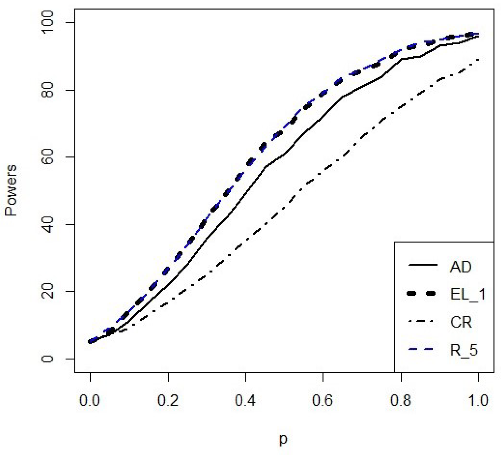
Figure 1 displays the local powers of A D , E L n , 1 , C R and R n , 5 over the complete range of mixture probabilities. The superior performance of E L n , 1 and R n , 5 , for this mixture distribution, is clear from this figure.
For the transformed data, K S ˜ n exhibits the lowest powers overall and H M n , 0.75 has the highest overall powers for the majority of the alternatives considered.
We will now consider the performance of the tests, developed specifically for the Rayleigh distribution, in general against all of the general alternative distributions listed in Table 1. From both Table 4 and Table 5 we see that, in general, the powers of K S n and C R n are lower for the majority of the alternatives considered and perform unfavourably in comparison to the other tests, for both sample sizes. On the other hand, E L n , 1 and R n , 5 perform quite well as we find that they outperform the other tests, having the highest estimated power for the majority of the alternatives considered. All tests considered perform quite well against the standard exponential distribution (which has a constant hazard rate) for both sample sizes.
Shifting our attention now to results associated with alternatives with increasing hazard rates, one finds, once again, that K S n and C R n have lower powers for both sample sizes considered. For most of the alternatives in this category E L n , 1 and R n , 5 have the highest power, only being outperformed, or equaled, for a handful of these alternatives by other tests.
Moving our attention to alternatives with a decreasing hazard, we see that all the tests considered perform very well and, since there are such minor differences in the power performance between all the tests, it is difficult to identify a single ‘best’ test for this set of alternatives. However, for the smaller sample size, K S n still attains powers that are slightly lower than the rest of the tests.
We now observe the results associated with alternatives with non-monotone hazard rates. The tests that generally perform well are A D n , E L n , 1 and R n , 1 . However, the test that exhibits the highest power for the majority of the alternatives, for both sample sizes, is R n , 5 .
Finally, we consider the performance of the tests for exponentiality based on the transformed data. The tests with the lowest powers are K S ˜ n and C M ˜ n . B H n , 1 and H M n , 1.25 perform very well, exhibiting high powers for most of the alternatives considered, especially for alternatives with decreasing or non-monotone hazard rates. H M n , 0.75 displays the highest overall powers for the majority of the alternatives considered. However, the highest estimated power, against all alternative distributions considered, is obtained by one of the tests specifically developed for the Rayleigh distribution and not by any of the exponentiality tests based on the transformed data. Therefore, we recommend that the tests proposed specifically for the Rayleigh distribution is used when goodness-of-fit testing is performed for the Rayleigh distribution.
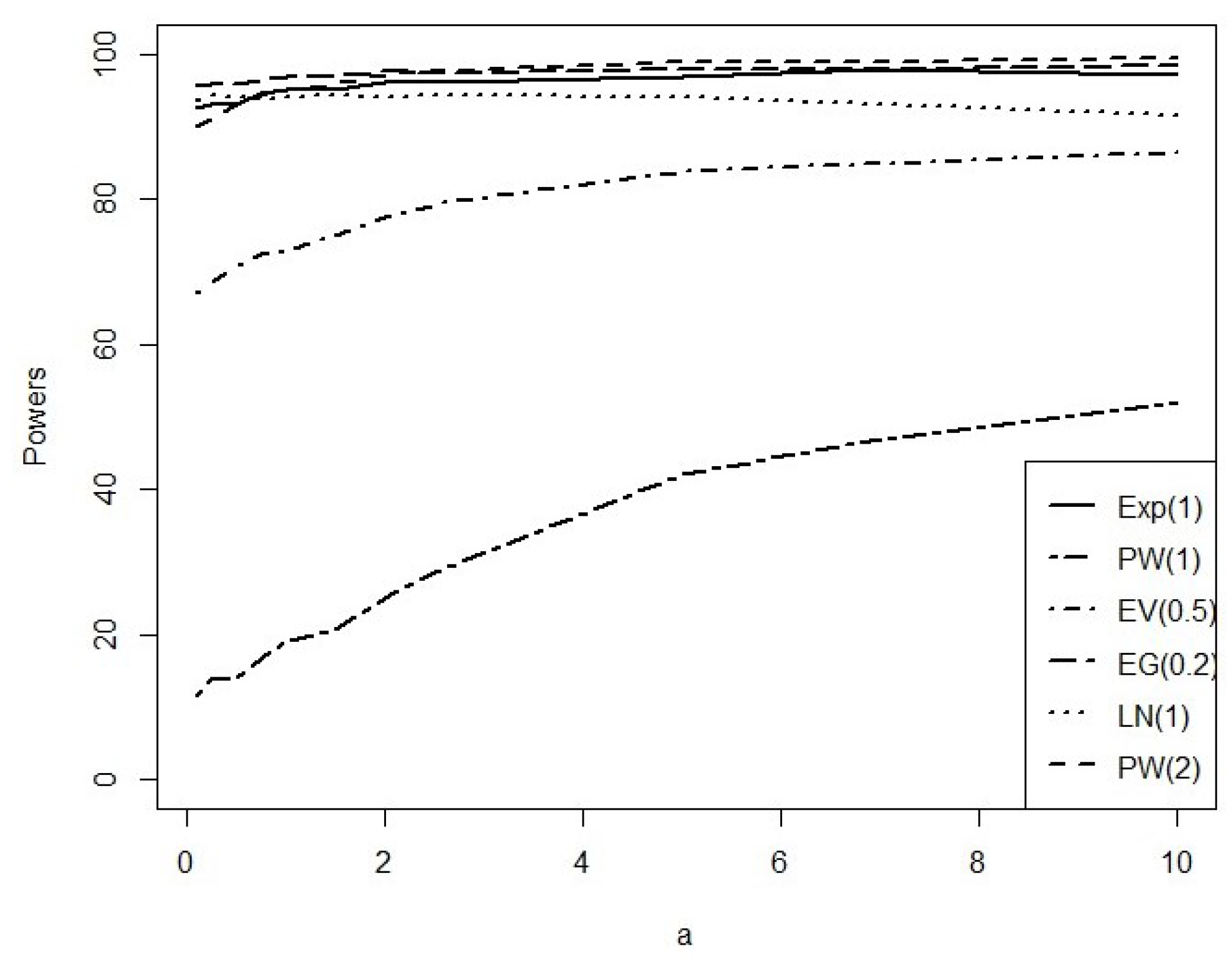
To conclude, we provide a brief demonstration of how the choice of the tuning parameter, a, influences the powers of the newly proposed test. In order to visualise the behaviour of the powers for different values of a, Figure 2 present the powers for R n , a over a grid of a values and six different alternative distributions. This figure is also used to motivate the choice of a values included in the study.
The choice of a = 1 was made since it is the point where the powers for most of the alternative distributions start to stabilize and reach a plateau. The choice for a = 5 is due to the fact that it is the point where the powers for most of the alternative distributions reach their maximum value.

5. Practical Application

As noted in Section 1, the Rayleigh distribution found various applications in the fields of survival analysis and reliability theory. In this section we demonstrate the use of the tests specifically developed for the Rayleigh distribution by applying them to a real-world survival data set: the COVID-19 data set of Italy given in Table 8—for a discussion on the data set, see [30]. The data set displays the COVID-19 mortality rates recorded for 59 days in Italy from 27 February 2020 to 27 April 2020. Ref. [30] discussed and analysed the use of an extended three parameter Rayleigh distribution to model the data. They concluded that the newly extended Rayleigh distribution is a good fit to the data. We, however, will investigate the goodness-of-fit of the traditional one parameter Rayleigh distribution as well as that of the exponential distribution. Figure 3 represents the probability plots of both the Rayleigh (grey dots) and exponential (black dots) distribution fitted to the data, where θ ^ = 6.583 and λ ^ = 0.123 in the case of the exponential distribution.
The probability plot suggests that the underlying distribution of the data might be the Rayleigh distribution instead of the exponential distribution.
Table 9 contains the estimated p-value (calculated based on 50,000 samples of size 59 simulated from the standard Rayleigh distribution) of each test for testing formally whether the data originated from a Rayleigh distribution.
From these p-values it is clear that all the tests do not reject the null hypothesis in (3) at a 5% significance level and we can therefore conclude that the Rayleigh distribution is also a feasible option to model the data.
Having found that the Rayleigh distribution is a good fit to the observed data, one can now go about calculating quantiles, moments and other useful distributional properties by using the theoretical Rayleigh distribution with estimated parameter θ ^ = 6.583 . For example, by fitting this Rayleigh distribution we find that the mean mortality rate over the 59 days is 8.2506 .

6. Conclusions and Future Research

In this article, a new goodness-of-fit test statistic specifically designed for the Rayleigh distribution was considered. The finite-sample performance of this newly suggested test was studied via the use of a Monte Carlo simulation. From the results, it is clear that this new test is not only feasible when testing goodness-of-fit for the Rayleigh distribution, it also outperforms or equals competitor tests for the majority of the alternative distributions considered. For practical implementation we suggest using the choice a = 5 for R n , a . Alternatively, one can use a data-dependent choice of this tuning parameter suggested, e.g., in [31].
In analysing mortality or survival data (like the COVID-19 data set) one will, more often than not, deal with observations that are censored. For our newly proposed test to be applicable in these kinds of situations, it needs to be modified to accommodate censoring. Naturally, this modification will complicate some of the asymptotic derivations and might be an avenue for future research. Some work in this regard has been started by [32] as well as [33].

Author Contributions

The authors (G.L.G., E.B., J.S.A.) contributed equally. All authors have read and agreed to the published version of the manuscript.

Funding

This research received no external funding.

Institutional Review Board Statement

Not applicable.

Informed Consent Statement

Not applicable.

Data Availability Statement

Not applicable.

Acknowledgments

The work of E. Bothma and J.S. Allison are based on research supported by the National Research Foundation (NRF). Any opinion, finding and conclusion or recommendation expressed in this material is that of the authors and the NRF does not accept any liability in this regard.

Conflicts of Interest

The authors declare no conflict of interest.

References

  1. Johnson, N.L.; Kotz, S.; Balakrishnan, N. Continuous Univariate Distributions, 2nd ed.; Wiley: New York, NY, USA, 1994. [Google Scholar]
  2. Rayleigh, F.R.S. Xii. On the resultant of a large number of vibrations of the same pitch and of arbitrary phase. Lond. Edinb. Dublin Philisophical Mag. J. Sci. 1880, 10, 73–78. [Google Scholar] [CrossRef] [Green Version]
  3. Dyer, D.; Whisenand, C. Best linear unbiased estimator of the parameter of the Rayleigh distribution. IEEE Trans. Reliab. 1973, 22, 229–231. [Google Scholar] [CrossRef]
  4. Polovko, A. Fundamentals of Reliability Theory; Academic Press: Cambridge, MA, USA, 1968. [Google Scholar]
  5. Brummer, M.; Mersereau, R.; Eisner, R.; Lewine, R. Automatic detection of brain contours in MRI data sets. IEEE Trans. Med. Imaging 1993, 12, 153–166. [Google Scholar] [CrossRef] [PubMed]
  6. Sijbers, J.; Poot, D.; den Dekker, A.; Pintjens, W. Automatic estimation of the noise variance from the histogram of a magnetic resonance image. Phys. Med. Biol. 2007, 52, 1335–1348. [Google Scholar] [CrossRef]
  7. Rajan, J.; Poot, D.; Juntu, J.; Sijbers, J. Segmentation Based Noise Variance Estimation from Background MRI Data; ICIAR 2010 Part I LNCS; Springer: Berlin/Heidelberg, Germany, 2010; Volume 6111, pp. 62–70. [Google Scholar]
  8. Guemana, M.; Hafaifa, A.; Mohamed, B.R. Reliability modeling using Rayleigh distribution: Industrial pump application. In Proceedings of the 19th European Conference on Mathematics for Industry ECMI2016, Santiago de Compostela, Spain, 13–17 June 2016. [Google Scholar]
  9. Elviana, E.; Purwadi, J. Parameters Estimation of Rayleigh Distribution in Survival Analysis on Type II Censored Data Using the Bayesian Method; Journal of Physics: Conference Series; IOP Publishing: Bristol, UK, 2020; Volume 1503, p. 012004. [Google Scholar]
  10. Meintanis, S.G.; Iliopoulos, G. Tests of fit for the Rayleigh distribution based on the empirical Laplace transform. Ann. Inst. Stat. Math. 2003, 55, 137–151. [Google Scholar] [CrossRef]
  11. Baratpour, B.S.; Khodadadi, F. A cumulative residual entropy characterization of the Rayleigh distribution and related goodness-of-fit test. J. Stat. Res. Iran 2012, 9, 115–1294. [Google Scholar] [CrossRef] [Green Version]
  12. Alizadeh Noughabi, R.; Alizadeh Noughabi, H.; Ebrahimi Moghaddam Behabadi, A. An entropy test for the Rayleigh distribution and power comparison. J. Stat. Comput. Simul. 2014, 84, 151–158. [Google Scholar] [CrossRef]
  13. Safavinejad, M.; Jomhoori, S.; Alizadeh Noughabi, H. A density-based empirical likelihood ratio goodness-of-fit test for the Rayleigh distribution and power comparison. J. Stat. Comput. Simul. 2015, 85, 3322–3334. [Google Scholar] [CrossRef]
  14. Nikitin, Y.Y. Tests based on characterizations, and their efficiencies: A survey. arXiv 2017, arXiv:1707.01522. [Google Scholar] [CrossRef] [Green Version]
  15. Betsch, S.; Ebner, B. Characterizations of continuous univariate probability distributions with applications to goodness-of-fit testing. arXiv 2018, arXiv:1810.06226. [Google Scholar]
  16. Stein, C. A bound for the error in the normal approximation to the distribution of a sum of dependent random variables. In Proceedings of the Sixth Berkeley Symposium on Mathematical Statistics and Probability, Berkeley, CA, USA, 9–22 July 1971; Volume 2: Probability Theory. University of California Press: Berkeley, CA, USA, 1972; Volume 6, pp. 583–603. [Google Scholar]
  17. Betsch, S.; Ebner, B. Testing normality via a distributional fixed point property in the Stein characterization. TEST 2018, 29, 105–138. [Google Scholar] [CrossRef] [Green Version]
  18. Henze, N.; Meintanis, S.G.; Ebner, B. Goodness-of-fit tests for the gamma distribution based on the empirical Laplace transform. Commun.-Stat.-Theory Methods 2012, 41, 1543–1556. [Google Scholar] [CrossRef]
  19. Allison, J.S.; Pretorius, C. A Monte Carlo evaluation of the performance of two new tests for symmetry. Comput. Stat. 2017, 32, 1323–1338. [Google Scholar] [CrossRef]
  20. Ledoux, M.; Talagrand, M. Probability in Banach Spaces: Isoperimetry and Processes; Springer Science & Business Media: Berlin/Heidelberg, Germany, 2013. [Google Scholar]
  21. Allison, J.S.; Santana, L.; Smit, N.; Visagie, I.J.H. An “apples-to-apples” comparison of various tests for exponentiality. Comput. Stat. 2017, 32, 1241–1283. [Google Scholar] [CrossRef] [Green Version]
  22. Henze, N.; Meintanis, S.G. Recent and classical tests for exponentiality: A partial review with comparisons. Metrika 2005, 61, 29–45. [Google Scholar] [CrossRef]
  23. Baringhaus, L.; Henze, N. Tests of fit for exponentiality based on a characterization via the mean residual life function. Stat. Pap. 2000, 41, 225–236. [Google Scholar] [CrossRef]
  24. Baringhaus, L.; Henze, N. A class of consistent tests for exponentiality based on the empirical Laplace transform. Ann. Inst. Stat. Math. 1991, 43, 551–564. [Google Scholar] [CrossRef]
  25. Henze, N.; Meintanis, S.G. Tests of fit for exponentiality based on the empirical Laplace transform. Statistics 2002, 36, 147–161. [Google Scholar] [CrossRef]
  26. Epps, T.; Pulley, L. A test of exponentiality vs. monotone-hazard alternatives derived from the empirical characteristic function. J. R. Stat. Soc. Ser. (Methodol.) 1986, 48, 206–213. [Google Scholar] [CrossRef]
  27. Allison, J.; Milošević, B.; Obradović, M.; Smuts, M. Distribution-free goodness-of-fit tests for the pareto distribution based on a characterization. Comput. Stat. 2022, 37, 403–418. [Google Scholar] [CrossRef]
  28. R Core Team. R: A Language and Environment for Statistical Computing; R Foundation for Statistical Computing: Vienna, Austria, 2019. [Google Scholar]
  29. Hlavac, M. Stargazer: Well-formatted regression and summary statistics tables. R Package Version 2018, 5, 2. [Google Scholar]
  30. Almongy, H.M.; Almetwally, E.M.; Aljohani, H.M.; Alghamdi, A.S.; Hafez, E. A new extended rayleigh distribution with applications of COVID-19 data. Results Phys. 2021, 23, 104012. [Google Scholar] [CrossRef]
  31. Allison, J.; Santana, L. On a data-dependent choice of the tuning parameter appearing in certain goodness-of-fit tests. J. Stat. Comput. Simul. 2015, 85, 3276–3288. [Google Scholar] [CrossRef]
  32. Bothma, E.; Allison, J.S.; Cockeran, M.; Visagie, I.J.H. Characteristic function and Laplace transform-based tests for exponentiality in the presence of random right censoring. Stat 2021, 10, e394. [Google Scholar] [CrossRef]
  33. Cuparić, M.; Milošević, B. New characterization based exponentiality tests for randomly censored data. arXiv 2020, arXiv:2011.07998. [Google Scholar] [CrossRef]
Figure 1. Local powers for some of the tests over the entire range of mixture probabilities of the Rayleigh exponential mixture distribution for n = 20.
Mathematics 10 01316 g001
Figure 2. Estimated powers for R 100 , a for some alternatives appearing in Table 1.
Mathematics 10 01316 g002
Figure 3. Probability plot of a fitted Rayleigh (grey dots) and exponential (black dots) distribution.
Mathematics 10 01316 g003
Table 1. Probability density functions of the alternative distributions considered in the Monte Carlo study.
Alternativef(x)Notation
Gamma 1 Γ ( θ ) x θ 1 exp ( x ) Γ ( θ )
Weibull θ x θ 1 exp ( x θ ) W ( θ )
Power 1 θ x ( 1 θ ) / θ , 0 < x < 1 P W ( θ )
Linear Failure Rate ( 1 + θ x ) exp x θ x 2 2 L F R ( θ )
Lognormal exp 1 2 log ( x ) θ 2 θ x 2 π 1 L N ( θ )
Inverse Gaussian θ 2 π x 3 1 / 2 exp θ ( x 1 ) 2 2 x I G ( θ )
Gompertz exp ( θ x ) exp 1 θ ( exp ( θ x ) 1 ) G O ( θ )
Exponential θ exp ( θ x ) E x p ( θ )
Extreme value 1 θ exp x + 1 exp ( x ) θ E V ( θ )
Exponential geometric ( 1 θ ) exp ( x ) ( 1 θ exp ( x ) ) 2 E G ( θ )
Table 2. Estimated local powers for the mixture of the Rayleigh and exponential distributions for various choices of the mixture parameter, p.
pn KS n CM n AD n EL n , 1 EL n , 5 CR n KL n , 3 KL n , 4 R n , 1 R n , 5 Exp
02055555555555
3054545455655
0.0520667877657 9 7
30678 9 8 9 668 9 8
0.1208812 15 101066101310
308914 16 13138713 16 12
0.152091117 20 15148814 20 14
30121421 25 19161211182317
0.220121422 27 1917111119 27 18
30151727 34 2521141525 34 23
0.2520151829 34 2521141424 34 25
30212436 44 3427192032 44 18
0.320192235 42 3024161530 42 30
30263044 54 41322527415342
0.3520222742 50 3730212237 50 36
30323754 62 49383132506149
0.420283248 56 4335262742 56 43
30414562 70 5844393857 70 57
0.4520343956 64 52413232496251
30465169 77 65524646647666
0.520394361 69 5745363655 69 57
30515976827257525371 83 72
Table 3. Estimated local powers for the mixture of the Rayleigh and exponential distributions, using transformed data, for various choices of the mixture parameter, p.
pn KS ˜ n CV ˜ n EP n BH n , 0.75 BH n , 1 BH n , 1.25 HM n , 0.75 HM n , 1 HM n , 1.25
020555555555
30555555555
0.052066 7 7 7 7 7 6 7
30677 8 7 8 777
0.12079 10 10 10 10 10 99
308101111 12 10 12 12 11
0.152081212 14 1313 14 1313
30101515 17 16 17 17 1616
0.220101516 18 1717 18 18 17
30141920 23 2222 23 2222
0.2520141820232222 25 2322
30182527313029 34 3131
0.320152324282826 30 2827
30233134403736 42 3938
0.3520192930353333 36 3434
30273840464444 49 4645
0.420233536413938 43 4140
30364649555452 57 5555
0.4520294143494646 51 4848
30425355636159 66 6362
0.520324647535251 57 5453
30476062706767 72 7069
Table 4. Estimated powers for general alternatives for the Rayleigh distribution for sample size n = 20 .
F KS n CM n AD n EL n , 1 EL n , 5 CR n KL n , 3 KL n , 4 R n , 1 R n , 5 Exp
CHR
E x p ( 1 ) 869096 97 9489848594 97 95
IHR
Γ ( 1.5) 576373757364444472 77 72
Γ ( 2 ) 32384443 46 411918444444
W ( 1.2) 646980847968545579 85 79
W ( 1.4) 374253585343262552 60 52
P W ( 1 ) 16204042132145 46 184121
L F R ( 2 ) 384563 70 56423636566959
L F R ( 4 ) 262947 56 41292525405542
E V ( 0.5) 566179 84 7458545573 84 76
E V ( 1.5) 222446 56 3320262835 56 38
G O ( 0.5) 566279 84 7457545475 84 76
G O ( 1.5) 222544543320272933 55 38
DHR
Γ ( 0.4) 100 100 100 100 100 100 100 100 100 100 100
Γ ( 0.7) 9798 100 100 9997989899 100 99
W ( 0.8) 9798 100 100 100 989898 100 100 100
E G ( 0.2) 949699 100 99959595989698
E G ( 0.5) 97989988 100 979898927199
E G ( 0.8) 86909555 100 99 100 99756094
NMHR
P W ( 2 ) 878998 99 9383969695 99 95
P W ( 3 ) 9999 100 100 100 99 100 100 99 100 100
L N ( 0.8) 67717266 75 745150 75 6875
L N ( 1 ) 90929493 95 928282949494
L N ( 1.5) 100 100 100 100 100 100 9999 100 100 100
I G ( 0.5) 9798989898979493 99 9898
I G ( 1.5) 5661604862 64 4242 64 5263
Table 5. Estimated powers for general alternatives for the Rayleigh distribution for sample size n = 30 .
F KS n CM n AD n EL n , 1 EL n , 5 CR n KL n , 3 KL n , 4 R n , 1 R n , 5 Exp
CHR
E x p ( 1 ) 969899 100 9997969699 100 99
IHR
Γ ( 1.5) 768187898879636588 90 87
Γ ( 2 ) 4753575659542828 60 5759
W ( 1.2) 818692949283747691 95 92
W ( 1.4) 535869726956373968 74 68
P W ( 1 ) 22285551143766 68 245027
L F R ( 2 ) 535976837153515372 84 74
L F R ( 4 ) 364361 69 55373737546856
E V ( 0.5) 748090 94 8872717388 94 89
E V ( 1.5) 323558684223394146 69 51
G O ( 0.5) 747891 94 8872737488 94 89
G O ( 1.5) 333758 68 4425414247 68 51
DHR
Γ ( 0.4) 100 100 100 100 100 100 100 100 100 100 100
Γ ( 0.7) 100 100 100 100 100 100 100 100 100 100 100
W ( 0.8) 100 100 100 100 100 100 100 100 100 100 100
E G ( 0.2) 9999 100 100 100 99 100 999996100
E G ( 0.5) 100 100 100 87 100 100 100 100 9368100
E G ( 0.8) 96989952 100 100 9999755999
NMHR
P W ( 2 ) 9798 100 100 9894 100 100 99 100 99
P W ( 3 ) 100 100 100 100 100 100 100 100 99 100 100
L N ( 0.8) 8386878188877071 89 8288
L N ( 1 ) 9798 99 99 99 989495 99 99 99
L N ( 1.5) 100 100 100 100 100 100 100 100 100 100 100
I G ( 0.5) 100 100 100 100 100 100 9999 100 100 100
I G ( 1.5) 7377776278796262 80 6780
Table 6. Estimated powers for general alternatives for the exponential distribution for sample size n = 20 .
F KS ˜ n CV ˜ n EP n BH n , 0.75 BH n , 1 BH n , 1.25 HM n , 0.75 HM n , 1 HM n , 1.25
CHR
E x p ( 1 ) 829090949393 95 9493
IHR
Γ ( 1.5) 526668 72 7170 72 7171
Γ ( 2 ) 2940434343434343 44
W ( 1.2) 577072777776 79 7876
W ( 1.4) 314446 52 5050 52 52 51
P W ( 1 ) 12117171411 21 1714
L F R ( 2 ) 304346555352 59 5754
L F R ( 4 ) 203031403636 42 3939
E V ( 0.5) 486162727168 76 7271
E V ( 1.5) 152122343027 38 3533
G O ( 0.5) 476263727168 76 7271
G O ( 1.5) 142223332928 38 3431
DHR
Γ ( 0.4) 100 100 100 100 100 100 100 100 100
Γ ( 0.7) 959898 99 99 99 99 99 99
W ( 0.8) 96989899999910010099
E G ( 0.2) 919595 98 98 97 98 98 98
E G ( 0.5) 959898 99 99 99 99 99 99
E G ( 0.8) 829090939393 94 94 93
NMHR
P W ( 2 ) 758479939189 95 9392
P W ( 3 ) 979998 100 100 99 100 100 100
L N ( 0.8) 64737474 75 75 727373
L N ( 1 ) 889393 94 94 94 94 94 94
L N ( 1.5) 99 100 100 100 100 100 100 100 100
I G ( 0.5) 96 98 98 98 98 98 98 98 98
I G ( 1.5) 53 64 64 626363585961
Table 7. Estimated powers for general alternatives for the exponential distribution for sample size n = 30 .
F KS ˜ n CV ˜ n EP n BH n , 0.75 BH n , 1 BH n , 1.25 HM n , 0.75 HM n , 1 HM n , 1.25
CHR
E x p ( 1 ) 959898 99 99 99 99 99 99
IHR
Γ ( 1.5) 738284 87 8685 87 86 87
Γ ( 2 ) 43575857 59 59 585758
W ( 1.2) 788787919090 92 9191
W ( 1.4) 476062676665 68 68 66
P W ( 1 ) 17156211814 27 2218
L F R ( 2 ) 445860686766 74 7068
L F R ( 4 ) 314344535148 56 5451
E V ( 0.5) 677980878684 89 8787
E V ( 1.5) 223029454137 51 4642
G O ( 0.5) 677879878584 89 8886
G O ( 1.5) 223129464239 51 4744
DHR
Γ ( 0.4) 100 100 100 100 100 100 100 100 100
Γ ( 0.7) 100 100 100 100 100 100 100 100 100
W ( 0.8) 100 100 100 100 100 100 100 100 100
E G ( 0.2) 999999 100 100 100 100 100 100
E G ( 0.5) 100 100 100 100 100 100 100 100 100
E G ( 0.8) 95989899 99 99 99 99 99
NMHR
P W ( 2 ) 939691 99 9897 99 99 98
P W ( 3 ) 100 100 100 100 100 100 100 100 100
L N ( 0.8) 8288 89 888888868788
L N ( 1 ) 9798 99 99 99 99 99 99 99
L N ( 1.5) 100 100 100 100 100 100 100 100 100
I G ( 0.5) 99 100 100 100 100 100 100 100 100
I G ( 1.5) 72 80 80 7878 80 737576
Table 8. COVID-19 data set of Italy.
1.518 2.450 2.508 2.686 2.780 2.814 2.881 3.134 3.148 3.341
3.564 3.606 3.827 4.011 4.040 4.253 4.408 4.416 4.571 4.639
4.640 4.859 5.073 5.452 6.194 6.503 7.201 7.214 7.407 7.445
8.479 8.646 8.697 8.905 8.906 8.961 9.037 10.138 10.282 10.644
10.908 10.919 11.010 11.273 11.410 11.775 11.822 11.950 12.396 13.226
13.333 14.242 14.330 15.137 15.787 16.046 16.561 17.337 18.474
Table 9. p-values for the COVID-19 data of Italy.
TestStatistic KS n CM n AD n EL n , 1 EL n , 5 CR n KL n , 3 KL n , 4 R n , 1 R n , 5
p-value0.059740.120380.129060.627860.56790.41040.096040.070.89030.91866
Publisher’s Note: MDPI stays neutral with regard to jurisdictional claims in published maps and institutional affiliations.

