Lightweight Image Super-Resolution Based on Local Interaction of Multi-Scale Features and Global Fusion

Abstract

In recent years, computer vision technology has been widely applied in various fields, making super-resolution (SR), a low-level visual task, a research hotspot. Although deep convolutional neural network has made good progress in the field of single-image super-resolution (SISR), its adaptability to real-time interactive devices that require fast response is poor due to the excessive amount of network model parameters, the long inference image time, and the complex training model. To solve this problem, we propose a lightweight image reconstruction network (MSFN) for multi-scale feature local interaction based on global connection of the local feature channel. Then, we develop a multi-scale feature interaction block (FIB) in MSFN to fully extract spatial information of different regions of the original image by using convolution layers of different scales. On this basis, we use the channel stripping operation to compress the model, and reduce the number of model parameters as much as possible on the premise of ensuring the reconstructed image quality. Finally, we test the proposed MSFN model with the benchmark datasets. The experimental results show that the MSFN model is better than the other state-of-the-art SR methods in reconstruction effect, computational complexity, and inference time.

1. Introduction

Single-image super-resolution (SISR) refers to the process of recovering a natural and clear high-resolution (HR) image from a low-resolution (LR) image. SISR has a wide range of applications in the real world, which are often used to improve the visual quality of images [1] and the performance of other high-level vision tasks [2], especially in the fields of satellite and aerial imaging [3,4,5], medical imaging [6,7,8], ultrasound imaging [9], and face recognition [10] etc. However, since different HR images can be downsampled to the same LR image, as a result, the incompatibility makes SISR still a challenging task.

In recent years, with the continuous improvement of computer learning capabilities, deep neural networks, especially methods based on convolutional neural networks, have been widely used in SISR, which has greatly promoted the development of image reconstructions. Dong et al. [11] first introduced a convolutional neural network (CNN) into the field of SR images, and proposed a super-resolution convolutional neural network (SRCNN). However, as the input LR image needs to be preprocessed by bicubic interpolation, the computational complexity is increased, and the high-frequency details in the original image are lost, which limit the efficiency of image reconstruction. Shi et al. [12] proposed an efficient sub-pixel convolutional neural network (ESPCN), which effectively replaces the bicubic interpolation preprocessing with a sub-pixel convolutional algorithm for upsampling operation, thereby reducing the overall computational complexity and avoiding the checkerboard effect caused by the deconvolution layer. In pursuit of better model performance, Zhang et al. [13] proposed the very deep residual channel attention network (RCAN) based on ESPCN, which stacks a large number of residual blocks and local connections to obtain better reconstruction quality.

It is found that increasing the network depth can improve the quality of image reconstruction, but it also leads to a substantial increase in the number of model parameters, and it also makes the training model more complicated. To solve this problem, Tai et al. [14] added a recursive block to the neural network to reduce model parameters, constructed a deep recursive residual network (DRRN), and transmitted the residual information through a combination of global learning and local learning to reduce the difficulty of training. DRRN uses a shared parameter strategy to reduce the parameters, but, in fact, it requires a huge amount of calculation to reconstruct the image. Hui et al. [15] proposed an information distillation network (IDN) which divides the features into two parts, with one part retained and the other part continuing to be used to extract information; thus, the model parameters are reduced under the premise of ensuring the quality of reconstruction quantity. Liu et al. [16] proposed a residual feature distillation network (RFDN) based on residual learning. The network retains the original features of the image without introducing additional parameters through residual connection, but the obtained feature map lacks related information of local features. Based on RFDN, this paper strips the channels with rich information features in the model, and pays more attention to the multi-scale channel information of the original image and the associated information of the local area. The main work of this paper is as follows:

• We propose a lightweight image super-resolution reconstruction network based on local feature channels and global connection mechanism, which separates the channels in the model and retains the channel features with rich spatial information. Our model significantly reduces the number of model parameters.
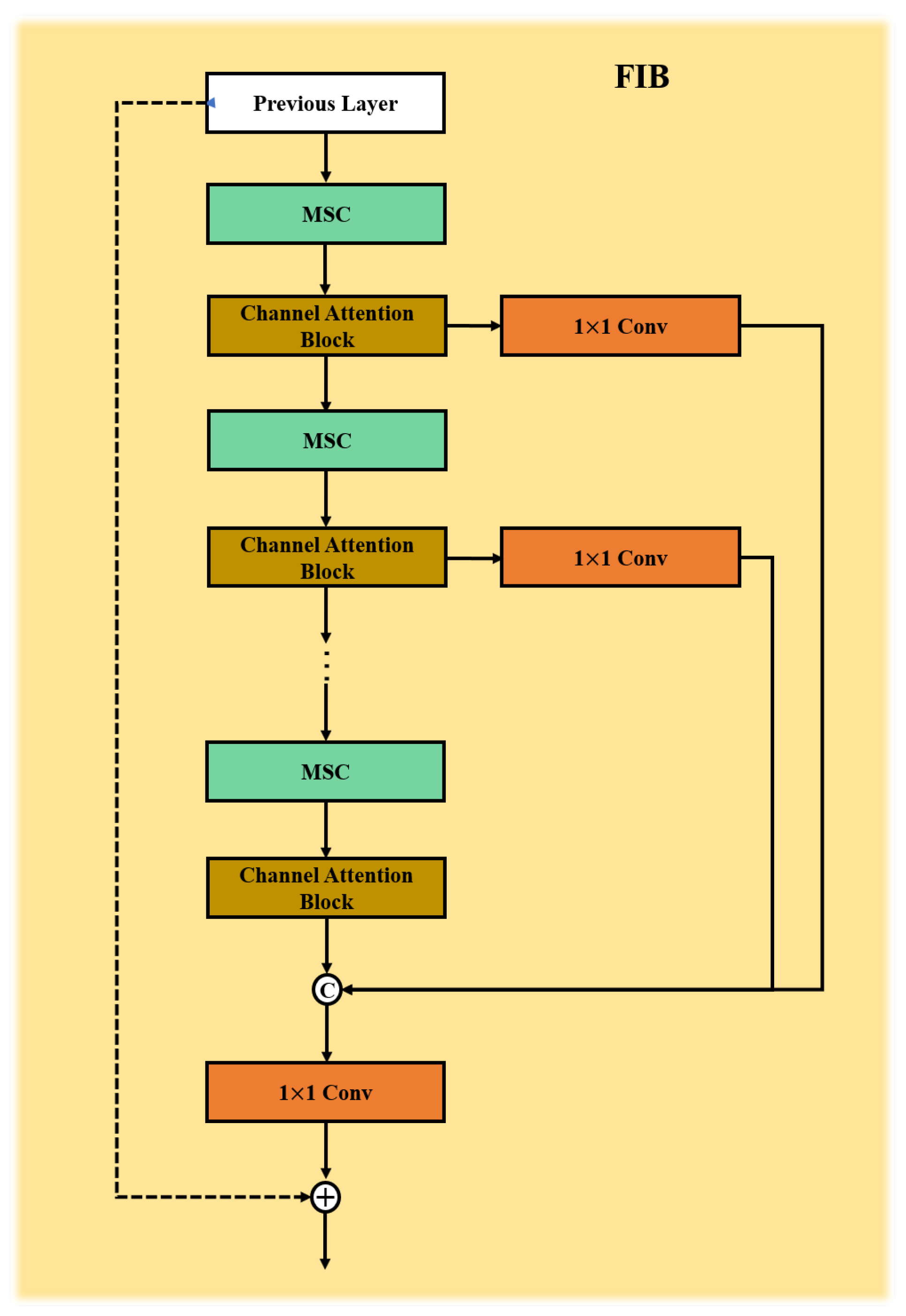
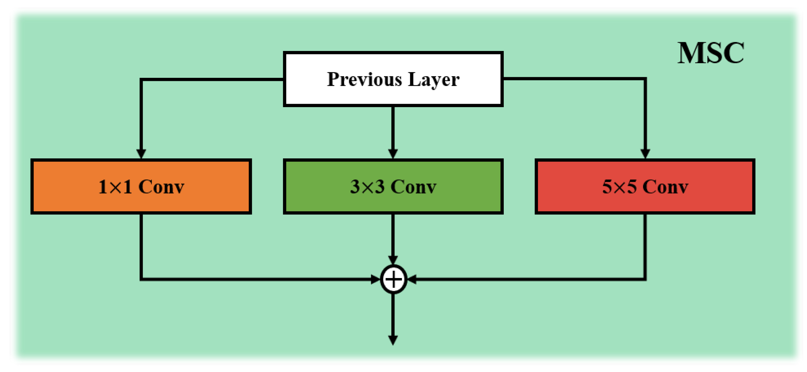
• We construct a feature fusion block based on local interaction of multi-scale features, which includes channel attention mechanism and multi-scale local feature interaction mechanism. The multi-scale local feature interaction mechanism is mainly composed of feature interaction blocks, through which local attention and interaction can effectively improve the authenticity of the reconstructed image compared with the original image, and realize the connection and fusion of multi-scale features.
• We use residual learning and global connection to fuse local features and global features, retain the high-frequency information and edge details of the original image, and improve the quality of the reconstructed image. As shown in Figure 1, on the Urban100 test set with scaling factor ×4, the PSNR of the reconstructed image of the MSFN model reaches 26.34 dB. Compared with the models CARN and SRMDNF of the same size, the reconstruction effect of our model is greatly improved.

2. Related Work

In recent years, the super-resolution of single image has been studied extensively [17,18,19]. We present an overview of the deep CNN for image super-resolution in Section 2.1. In order to reduce model parameters and speed up image reasoning, lightweight image super-resolution models have been widely studied. We will elaborate on this part in Section 2.2.

2.1. Deep CNN for Image Super-Resolution

Dong et al. [11] used end-to-end convolutional neural network (SRCNN) for the first time to extract, map, and reconstruct image features, and found that the reconstruction effect exceeded the traditional image super-resolution (SR) method. However, the network structure is simple and the correlation between low-resolution (LR) image and original image is not considered. Some researchers started with the depth of the network, hoping to fully extract the relevant information between images through the deep network model. Kim et al. [20] proposed a very deep super-resolution (VDSR) convolutional network based on the global residual learning method, which not only improves the reconstruction effect, but also accelerates the network convergence speed. Haris et al. [21] proposed a deep back-projection network (DBPN) for super-resolution with iterative up–down sampling, which provides timely feedback of the error mapping at each stage, and performs better, especially in large-scale images. Yang et al. [22] used skip connections to increase the number of network layers, which enhanced the feature expression ability of the network and made the reconstructed image closer to the real image. Lim et al. [23] removed the batch specification layers that affected the reconstruction effect in an enhanced deep super-resolution network (EDSR), and stacked more convolutional layers to achieve better performance of the model. In order to improve the visual effect of reconstructed images, Yang et al. [24] constructed a multi-level feature extraction module using dense connections, which can obtain richer hierarchical feature images. With the deepening of the network structure, the number of parameters and the computational complexity of this type of model increase greatly, limiting its application in the real world.

2.2. Lightweight CNN for Image Super-Resolution

In order to reduce the number of model parameters, the complexity, and training difficulty of network calculation, researchers began to improve the deep network, compressing the model by sharing parameters, residual learning, attention mechanism, and information distillation, and proposed a lightweight image reconstruction network based on CNN. Kim et al. [25] used a deep recursive structure in the deep recursive convolutional network (DRCN) to share parameters, but the model performance was degraded compared with VDSR in some test sets, and the actual amount of computation of the model did not decrease accordingly. Tai et al. [14] proposed a deep recursive residual network (DRRN)-based DRCN, which reduces storage cost and computational complexity by global connection of multipath residual information. Li et al. [26] added an adaptive weighted block in residual learning to fully extract image features and effectively limit the number of model parameters. Hu et al. [27] introduced channel attention mechanism into a deep neural network, and added weight to the features of each output channel in the convolution operation to reasonably allocate limited computer resources, so as to obtain a wide application in the lightweight network architecture. Hui et al. [28] proposed an information distillation network, which uses a combination of embedding loss and information distillation to solve the problem of image recognition. They used a small-size convolution kernel to compress network parameters and reduce the computational cost and complexity of the training model. Tian et al. [29] proposed heterogeneous structure in information extraction and enhancement blocks, which greatly reduced the computational cost and memory consumption. Hui et al. [15] used convolution kernels with sizes of 1 × 1 and 3 × 3 to enhance the extracted features, which made the model have better image reconstruction performance and inference speed. Jiang et al. [30] constructed a sparse perceptive attention module based on pruning, which can reduce the model size without a noticeable drop in performance. However, these methods cannot make full use of the associated information between the original image and the low-resolution (LR) image, and the interaction of information between different regions has not been paid enough attention. Based on this, we adopt a fusion block based on multi-scale feature local interaction to fully extract the feature information in the original image. In addition, we strip and compress the channels, and make a trade-off between the performance and the inference speed, which effectively improves the comprehensive performance of the model.

3. Proposed Method

3.1. Network Architecture

In this paper, we propose a lightweight image reconstruction network based on local interaction of multi-scale features, and use local interaction of multi-scale features and the global connection of comparative residuals to learn second-order feature statistics in order to obtain more representative features. The network structure we propose mainly includes five parts: shallow feature extraction block, deep feature extraction block based on multi-scale interaction mechanism, global feature fusion block, upsampling block, and image reconstruction block, as shown in Figure 2.

As shown in Equation (1), $I_{LR}$ represents the input image, and the network uses a convolution layer to extract the shallow features of the input image $I_{LR}$. The shallow feature extraction block can be expressed as follows:

$$X_{SF}=F_{SF}(I_{LR})$$

(1)

where $F_{SF}(·)$ represents a simple single-layer convolution mapping, which aims to achieve shallow feature extraction. The shallow feature $X_{SF}$ is extracted through single-layer convolution, and then $X_{SF}$ is input into the deep feature extraction block based on multi-scale interaction mechanism to obtain the high-dimensional feature $X_{PF}$ after feature mapping, which is expressed as Equation (2):

$$X_{PF}=F_{DPAM}(X_{SF})$$

(2)

The deep feature extraction block is composed of M feature interaction blocks (FIBs) and M skip connections, where $F_{DPAM}(·)$ represents the mapping function corresponding to the deep feature extraction block, and $X_{SF}$ represents extracted feature maps with deep receptive fields. The features extracted from each FIB are first concatenated in the channel dimension in series to form new high-dimensional features, and then a single-convolution layer is used to reduce the dimensionality of the obtained high-dimensional features. Compared with the existing SISR methods, our feature extraction block based on the multi-scale feature interaction mechanism proposed in this paper can make the network more effectively use the extracted features and suppress invalid features. Moreover, this block can compare and fuse the receptive field information of different scales in the original image, fully retain the texture information of the low-resolution (LR) image, and effectively improve the quality of the reconstructed image. The features extracted from FIB are input into the global feature fusion block, and the feature information extracted at different stages is retained to the maximum extent by means of global connection. The fused feature $X_{GF}$ is shown in Equation (3):

$$X_{GF}=F_{GFF}([X_{P{F}_1},X_{P{F}_2}\cdots X_{P{F}_m}])$$

(3)

where $X_{P{F}_m}$ represents the high-dimensional feature extracted by the M-th FIB. The feature information extracted by the M FIBs is input into the mapping function $F_{GFF}(·)$ corresponding to the feature fusion block, and the feature information is spliced in the channel dimension to obtain the global feature $X_{GF}$ based on the entire network.

Then, the features after fusion and transformation are used as the input of upsampling block, and the input is upsampled by using the method of sub-pixel convolution [12] to obtain a high-resolution (HR) feature mapping. The features after upsampling are shown in Equation (4):

$$X_{SR}=F_{UP}^L(X_{GF})=PS(X_{GF})$$

(4)

$$PS(T_{x,y,c·r^2})=T_{rx,ry,c}$$

(5)

In the above Equation, $F_{UP}^L$(·) represents the upsampling operation based on sub-pixel convolution, and $X_{SR}$ represents the high-resolution (HR) feature map output after upsampling. At present, the commonly used upsampling methods in the field of super-resolution (SR) reconstruction include interpolation operation, transposed convolution operation, and sub-pixel convolution operation. The sub-pixel convolution operation achieves upsampling by rearranging pixels, reducing the amount of model parameters. Therefore, in order to make the network achieve better results in terms of reconstruction rate and accuracy, we choose to implement upsampling through sub-pixel convolution operation. In Equation (4), $PS(·)$ represents a periodic sorting operator, which rearranges the feature map with a size of H × W × C · r${}^2$ into a feature map with a shape of rH × rW × C. Equation (5) mathematically describes the subpixel upsampling operation, the effect of which is shown in Figure 3.

3.2. Multi-Scale Feature Interaction Block

In this section, we provide more details on the multi-scale FIB. The FIB is the main structure for feature mapping and local fusion in the network, which constructs N multi-scale feature interaction components (MSCs) and N channel attention blocks (CABs) for pixel information of different scales. The FIB structure is shown in Figure 4.

The input of each FIB needs to pass through the MSC to extract the feature information under the condition of multiple receptive fields. As shown in Equation (6), the output feature $X_{out}^{i-1}$ of the $i-1$th MSC is the input feature $X_{in}^i$ of the i-th MSC. $F_{MSC}^i$(·) is the mapping relationship corresponding to the i-th MSC, through which we can extract the interaction and spatial information of the regional features of $X_{in}^i$ at different scales, so that the high-frequency information and edge texture details of the input image relatively can be completely preserved by the feature $X_{out}^i$.

$$X_{out}^i=F_{MSC}^i(X_{in}^i)(X_{in}^i=X_{out}^{i-1})$$

(6)

The specific architecture of the MSC is shown in Figure 5. It can be seen that the MSC is mainly composed of three filters of different scales, and the convolution kernel sizes of the filter are 1 × 1, 3 × 3, and 5 × 5, respectively. MSCs enrich spatial information by expanding receptive fields, in which the large-scale filters are mainly used to extract feature attention information in different regions, and the small-scale filters are used to enhance the correlation degree between local regions. We pad the edge of the feature map with elements with zero pixel value to ensure that the size of the feature map remains unchanged after the convolution operation. When the size of the convolution kernel of the filter is 3 × 3 and 5 × 5, the corresponding edge filling scale is 1 and 2, respectively. When the size of the convolution kernel of the filter is 1 × 1, no edge filling is performed in the feature map.

The MSC uses filters of different scales to extract and enhance feature information, and the enhanced features are added pixel by pixel according to their weights to obtain a new feature map with rich spatial elements, as shown in Equations (7) [31], (8), and (9):

$$X_i=b_i+{\displaystyle \sum _{j=0}^{C_{in}-1}}{W}_i\times X_{pre}(i=1,2,3)$$

(7)

$$X_{MF}={\displaystyle \sum _{i=1}^3}{k}_i\times C_i\times X_i(k_i=1,i=1,2,3)$$

(8)

$$C_i=\frac{1}{|X_i|}(i=1,2,3)$$

(9)

In Equation (7), $W_1$, $W_2$, and $W_3$ represent the weight coefficients corresponding to filters with convolution kernel sizes 1 × 1, 3 × 3, and 5 × 5, respectively. As shown in Figure 6, convolution kernels of different scales focus on the correlation information between different regions of the same object, and then perform weighted summation for the extracted feature information. In Equation (9), $C_i$ represents the two-norm value of each feature vector, and each feature map is normalized by this value. In Figure 6, $k_1$, $k_2$, and $k_3$ represent the corresponding weight coefficients of feature information extracted from each convolution kernel, respectively. In this paper, $k_1$ = $k_2$ = $k_3$ = 1, which makes the extracted feature map $X_{MF}$ have rich spatial information features and regional interactions, and is helpful for the restoration and construction of key features and edge information in subsequent image reconstruction.

The features extracted by the feature interaction component are firstly input into the channel attention component, then the output result is input into the remaining $N-1$ MSCs and CABs for iterative optimization; finally, the features obtained at each stage are spliced in the channel dimension, and then the high-dimensional feature $X^i$ is obtained by residual connection with the initial input feature $X_{pre}$. Specifically, as shown in Equations (10) and (11):

$$X^i=F_{CAB}^i(F_{MSC}^i(\cdots F_{CAB}^1(F_{MSC}^1(X_{pre}))))(i=1,2,\cdots ,N)$$

(10)

$$X_t=F_{conv1}(Concat[F_{conv1}^i(X^1),\cdots ,F_{conv1}^{N-1}(X^{N-1})]+X^N)+X_{pre}$$

(11)

where $F_{MSC}^i(·)$ and $F_{CAB}^i(·)$ represent the relationship corresponding to the i-th MSC and CAB, respectively. We use a single convolutional layer to reduce the dimensionality of the feature maps $X^i$ obtained at each stage, then splice the dimension-reduced features in the channel dimension, and finally add the original feature $X_{pre}$ on the pixel-level dimension to obtain the final feature map $X_t$.

4. Experiments

In this section, we firstly test the influence of the number of FIBs and channels on the quality of the reconstructed image; secondly, we perform test experiments on SR benchmark datasets such as Set5 [32], Set14 [33], Urban100 [34], BSD100 [35], and Manga109 [36]; and then we use the peak signal-to-noise ratio (PSNR) and structural similarity (SSIM) of the Y-channel in YCbCr as quantitative indicators to compare the experimental data with other excellent super-resolution (SR) methods. Finally, we visualize the reconstruction results and analyze the reconstruction effects from a subjective visual perspective.

4.1. Training Settings

In order to compare with existing network algorithms, such as DRRN [14], CARN [37], MemNet [38], and IMDN [28], we use the same training dataset—the DIV2K dataset [39]. The dataset used in this paper includes a total of 800 training images, 100 validation images, and 100 test images, and contains rich scenes with rich edge and texture details. Meanwhile, we perform data enhancement on the training images [40] by using random rotation, horizontal flip, and small window slice to make the training data expand to eight times the original one, so that it can adapt to image reconstruction problems with different tilt angles.

In the training phase, we set batch size to 16, LR input size to 64 × 64, and the number of channels in the convolution layer to 48. The deep feature extraction block based on multi-scale feature interaction mechanism contains six FIBs, and each FIB contains four MSCs and four CABs. Among them, the selection of the number of channels and the numbers of FIBs will be explained in detail in Section 4.2 of this paper. Meanwhile, the model parameters are optimized using the Adam [41] algorithm, which are set to ${\beta }_1$ = 0.9, ${\beta }_2$ = 0.999, and $\epsilon ={10}^{-8}$. The learning rate is initially set to ${10}^{-3}$ by using weight normalization and then decreased to half each 200 epoch of back-propagation. All the experiments were completed on a computer with the following specifications: Intel i7-9700, 32 GB RAM, and NVIDIA GeForce RTX2080Ti 12 GB GPU.

4.2. Ablation Experiment

We first study the influence of the number of multi-scale feature interaction blocks (FIBs) in the model on the final experimental results, taking the DIK2K dataset as the training object, and then we test the quantitative indicators of the model on the Set14 dataset. The experimental results are shown in

Table 1. The influence of the number of FIBs on the model reconstruction effect.

Scale	Number of FIBs	Number of Channels	Params (K)	Set14
				PSNR (dB)	SSIM
4×	4	48	395	28.47	0.7789
	6		571	28.61	0.7814
	8		747	28.69	0.7824

and Figure 7.

In order to better understand the relationship between the number of FIBs and the quality of image reconstruction, we set the number of channels to 48, control the number, and keep parameters of other components in the model unchanged, and only change the number of FIBs. It can be seen from Table 1 that the image reconstruction quality is positively correlated with the number of FIBs. Here we set the scaling factor to four: it shows that when the number of FIBs increases from four to six, the model parameters are relatively increased by 176 K, and the PSNR of reconstructed images is relatively increased by 0.14, which indicates that the reconstruction quality has been significantly improved. When the number of FIBs increases from six to eight, the SSIM value of the reconstructed image is improved to 0.7824. The influence curves of the number of FIBs on the LOSS value, PSNR value, and SSIM value of reconstruction results are shown in Figure 7a–c. As the number of FIBs increases, the LOSS value of reconstructed image relative to the original image decreases, while the value of quantitative indicators such as PSNR and SSIM increases.

In order to verify the influence of the number of channels in the FIB on the reconstruction quality of the model, we perform comparative experiments on models with different numbers of channels. It can be seen from

Table 2. The influence of the number of channels in the FIB on the model reconstruction effect.

Scale	Number of FIBs	Number of Channels	Params (K)	Set5
				PSNR (dB)	SSIM
4×	6	48	571	32.12	0.8941
		56	772	32.16	0.8947
		64	1004	32.23	0.8950

that as the number of channels increases, the reconstruction quality of the model for the Urban100 dataset increases, but the number of model parameters also increases sharply. When the number of channels is adjusted from 48 to 64, the number of the entire model parameters is greatly increased from 571 K to 1004 K, while the SSIM value is only increased by 0.0009. Figure 7d–f show the comparison of LOSS value, PSNR value, and SSIM value of models based on different number of channels on Set5 dataset, respectively. It can be found that although the image reconstruction quality can be improved by increasing the number of channels in FIB, the number of model parameters also increases sharply, as shown in Table 2. Therefore, from the perspective of model lightweight, the larger number of channels is not the better one, and it needs to be considered comprehensively in combination with the number of model parameters. As can be seen from Table 1 and Table 2 and Figure 7, when we set the number of FIBs to six and the number of channels to 48 after considering comprehensively, the model has the best comprehensive performance in terms of parameter number and reconstruction effect.

In order to further explore the operation mechanism of feature extraction from different-sized convolution kernels and their influence on reconstructed images, we stripped the feature map extracted from convolution layers of the first MSC at different scales in the second FIB and performed visual analysis on the separated features. Figure 8b shows that the small-scale convolution kernel pays more attention to the pixel information of the shallow layer, focusing on extracting the small-resolution features in the original image. By analyzing Figure 8c,d, we can find that the larger the size of the convolution kernel, the more global the extracted information, and the more attention is given to the relevance of local information. Therefore, using convolution kernels of different scales to extract and pay attention to spatial information of different levels has theoretical significance and practical effect in terms of visualized results.

4.3. Quantitative Analysis

We compared the proposed MSFN with commonly used baseline SR models with ×2, ×3, and ×4 scales, including SRCNN [11], FSRCNN [42], VDSR [20], LapSRN [43], DRRN [14], MemNet [38], LESRCNN [29], SRMDNF [44], SRDenseNet [45], CARN [37], and IMDN [28], and here we use PSNR and SSIM [46] as quantitative evaluation metrics. PSNR evaluates the distortion level between the image and the target image based on the error between the corresponding pixels. PSNR is the most common and widely used objective evaluation metric of images. In order to compare the reconstruction performance with the mainstream super-resolution algorithm, PSNR is selected as one of the quantitative evaluation metrics. However, since PSNR does not take into account the visual characteristics of human eyes, the evaluation results are often inconsistent with people’s subjective feeling. Therefore, we compare the reconstruction results of each algorithm on SSIM metric. SSIM is a full-reference image quality evaluation metric, which measures image similarity from the three aspects of brightness, contrast, and structure. SSIM is more consistent with the characteristics of human eye observation images in the objective world.

The specific results are shown in

Table 3. Average PSNR/SSIM value for scale factor ×2, ×3, and ×4 on datasets Set5, Set14, BSD100, Urban100, and Manga109.

Method	Scale	Params	Set5	Set14	BSD100	Urban100	Manga109
			PSNR/SSIM	PSNR/SSIM	PSNR/SSIM	PSNR/SSIM	PSNR/SSIM
Bicubic	2×	-	33.66/0.9299	30.24/0.8688	29.56/0.8431	26.88/0.8403	30.80/0.9339
SRCNN		57 K	36.66/0.9542	32.45/0.9067	31.36/0.8879	29.50/0.8946	35.60/0.9663
FSRCNN		13 K	37.05/0.9560	32.66/0.9090	31.53/0.8920	29.88/0.9020	36.67/0.9710
VDSR		666 K	37.53/0.9590	33.05/0.9130	31.90/0.8960	30.77/0.9140	37.22/0.9750
LapSRN		813 K	37.52/0.9591	33.08/0.9130	31.08/0.8950	30.41/0.9101	37.27/0.9740
DRRN		297 K	37.74/0.9591	33.23/0.9136	32.05/0.8973	31.23/0.9188	37.60/0.9736
MemNet		678 K	37.78/0.9597	33.28/0.9142	32.08/0.8978	31.31/0.9195	37.72/0.9740
LESRCNN		516 K	37.65/0.9586	33.32/0.9148	31.95/0.8964	31.45/0.9206	-/-
SRMDNF		1511 K	37.79/0.9601	33.32/0.9159	32.05/0.8985	31.33/0.9204	38.07/0.9761
CARN		1592 K	37.76/0.9590	33.52/0.9166	32.09/0.8978	31.92/0.9256	38.36/0.9764
IDN		715 K	37.83/0.9600	33.30/0.9148	32.08/0.8985	31.27/0.9196	-/-
IMDN		694 K	38.00/0.9605	33.63/0.9177	32.19/0.8996	32.17/0.9283	38.88/0.9774
MSFN-S		555 K	37.96/0.9603	33.61/0.9181	32.15/0.8988	32.14/0.9272	38.85/0.9772
MSFN		1568 K	38.01/0.9606	33.77/0.9193	32.24/0.9000	32.24/0.9286	38.97/0.9776
Bicubic	3×	-	30.39/0.8682	27.55/0.7742	27.21/0.7385	24.46/0.7349	26.95/0.8556
SRCNN		8 K	32.75/0.9090	29.30/0.8215	28.41/0.7863	26.24/0.7989	30.48/0.9117
FSRCNN		13 K	33.18/0.9140	29.37/0.8240	28.53/0.7910	26.43/0.8080	31.10/0.9210
VDSR		666 K	33.67/0.9210	29.78/0.8320	28.83/0.7990	27.14/0.8290	32.01/0.9340
LapSRN		813 K	33.82/0.9227	29.87/0.8230	28.82/0.7980	27.07/0.8280	32.31/0.9350
DRRN		297 K	34.03/0.9244	29.96/0.8349	28.95/0.8004	27.53/0.8378	32.42/0.9359
MemNet		678 K	34.09/0.9248	30.00/0.8350	28.96/0.8001	27.56/0.8376	32.51/0.9369
LESRCNN		516 K	33.93/0.9231	30.12/0.8380	28.91/0.8005	27.70/0.8415	-/-
SRMDNF		1528 K	34.12/0.9254	30.04/0.8382	28.97/0.8025	27.57/0.8398	33.00/0.9403
CARN		1592 K	34.29/0.9255	30.29/0.8407	29.06/0.8034	28.06/0.8493	33.49/0.9440
IDN		715 K	34.11/0.9253	29.99/0.8354	28.95/0.8013	27.42/0.8359	-/-
IMDN		703 K	34.36/0.9270	30.32/0.8417	29.09/0.8046	28.17/0.8519	33.61/0.9445
MSFN-S		562 K	34.31/0.9265	30.33/0.8421	29.11/0.8053	28.22/0.8531	33.65/0.9451
MSFN		1574 K	34.47/0.9275	30.38/0.8428	29.20/0.8082	28.55/0.8549	33.71/0.9463
Bicubic	4×	-	28.42/0.8104	26.00/0.7027	25.96/0.6675	23.14/0.6577	24.89/0.7866
SRCNN		8 K	30.48/0.8628	27.50/0.7513	26.90/0.7101	24.52/0.7221	27.58/0.8555
FSRCNN		13 K	30.72/0.8660	27.61/0.7550	26.98/0.7150	24.62/0.7280	27.90/0.8610
VDSR		666 K	31.35/0.8830	28.02/0.7680	27.29/0.7260	25.18/0.7540	28.83/0.8870
LapSRN		813 K	31.54/0.8850	28.19/0.7720	27.32/0.7270	25.21/0.7560	29.09/0.8900
DRRN		297 K	31.68/0.8888	28.21/0.7720	27.38/0.7284	25.44/0.7638	29.18/0.8914
MemNet		678 K	31.74/0.8893	28.26/0.7723	27.40/0.7281	25.50/0.7630	29.42/0.8942
LESRCNN		516 K	31.88/0.8903	28.44/0.7772	27.45/0.7313	25.77/0.7732	-/-
SRMDNF		1552 K	31.96/0.8925	28.35/0.7787	27.49/0.7337	25.68/0.7731	30.09/0.9024
SRDenseNet		2015 K	32.02/0.8934	28.50/0.7782	27.53/0.7337	26.05/0.7819	-/-
CARN		1592 K	32.13/0.8937	28.60/0.7806	27.58/0.7349	26.07/0.7837	30.40/0.9082
IDN		715 K	31.82/0.8903	28.25/0.7730	27.41/0.7297	25.41/0.7632	-/-
IMDN		715 K	32.21/0.8948	28.58/0.7811	27.56/0.7353	26.04/0.7838	30.42/0.9074
MSFN-S		571 K	32.12/0.8941	28.61/0.7814	27.56/0.7348	26.02/0.7834	30.45/0.9075
MSFN		1583 K	32.26/0.8946	28.65/0.7815	27.62/0.7364	26.34/0.7906	30.58/0.9089

Red color indicates the best performance.

(the red text font represents the optimal results, the number of FIBs in the MSFN model and the MSFN-S model is set to six, the number of channels is set to 48, and the convolution kernel of MSC in the MSFN-S model is set to 1 × 1, 3 × 3, and 1 × 1, respectively).

It can be seen from Table 3 that when the scaling factor is 2, the PSNR value of the MSFN model proposed in this paper is increased by 0.25 dB, 0.25 dB, 0.15 dB, 0.32 dB, and 0.61 dB on the five datasets, respectively, compared with the CARN model of the same parameter scale; it also can be seen that the MSFN model is superior to the CARN model in reconstruction effect. When the scaling factor is 3, the number of parameters of the small-scale MSFN-S model is similar to that of the LESRCNN model, but the image reconstruction quality is much higher than that of the LESRCNN model. The test result on the BSD100 dataset is increased by 0.2 dB, which greatly improves the quality of the reconstructed image, so that the reconstructed image contains rich original information and texture details. When the scaling factor is 4, we screened out the model whose reconstruction quality exceeds 32.10 dB on Set5, among which the MSFN-S model has the smallest number of parameters, and the MSFN-S model obtains better results in the reconstruction tests of other datasets. With Manga109 as the test dataset, the SSIM value of the MSFN reconstructed image is the best in the larger model structure with more than 1000 K parameters, and the optimal value is 0.9089, which is improved by 0.0065 compared with the SRMDNF model of the same scale.

In order to understand the comprehensive performance of each model, we compare the amount of computational complexity required in the image reconstruction process, the inference time, and the PSNR value of the reconstruction result with those of the models such as LESRCNN [29], CARN [37], IMDN [28], and MSFN-S.

FLOPs stands for floating point operands and can be used to measure the complexity of algorithms and models. Equation (12) describes the theoretical concept of FLOPs mathematically [47]:

$$FLOPs=(2\times C_i\times K^2-1)\times H\times W\times C_o$$

(12)

$C_i$ and $C_o$ represent the input and output channels, respectively, K represents the size of the convolution kernel, and H and W represent the size of the output feature map. We randomly select an image from the Set14 dataset with a resolution of 528 × 656 as the test image. We input the image into each reconstruction model, and calculate the computational complexity required by the convolution layer in each model according to Equation (12). Meanwhile, we record the inference time and reconstruction effect in

Table 4. Complexity of five networks for SISR.

Method	FLOPs (G)	Time (ms)	PSNR (dB)
LESRCNN	77	44	26.37
CARN	41	62	26.57
IMDN	21	37	26.62
MSFN-S	18	31	26.67

. From the perspective of inference time, MSFN-S inference test image only takes 31 ms, while IMDN and CARN model need 37 ms and 62 ms to complete inference, respectively. From the perspective of image reconstruction quality, MSFN-S has the highest image quality, with which the value of PSNR reaches 26.67 dB. Therefore, the MSFN-S model is more efficient than the other three models in terms of information timeliness and reconstruction capability.

4.4. Qualitative Visual Analysis

Since quantitative indicators such as PSNR and SSIM do not pay attention to the continuity of local details and cannot fully reflect the image quality, we make a visual analysis of the reconstructed images of each model. Here, we use img005 in the Set14 dataset, img019 in the BSD100 dataset, img026 in the Urban100 dataset, and img093 in the Manga109 dataset for the analysis of visualization, with the results shown in Figure 9, from which we can see that the models SRCNN, DRRN, MemNet, and LESRCNN have weak ability to reconstruct edge information and lack relatively clear line information. For example, in the reconstruction result of the img005 image, the edge lines of the headwear are blurry, and the contours of small objects cannot be restored well, while the reconstructed image of the MSFN model has better line information. From the reconstructed image of img019 by MSFN, it can be seen that MSFN can better restore the details of the bifurcation in the upper left corner of the original image, while models such as CARN cannot. Compared with IMDN and other models, the MSFN model has improved its ability to recover key information of the original image. In the original image of img093, there is a black spot in the lower left corner of the eye. Only the MSFN model pays attention to the continuity of the global information and local details of the original image, so that the detailed information of the black spot is better reconstructed. By comparing the visualization results, it can be seen that the MSFN model has a certain improvement in image reconstruction effect compared with the existing models.

In order to verify the correctness more accurately of the subjective judgments of various reconstruction methods, we designed an image definition questionnaire that requires respondents to score the definition of the reconstruction results of each model according to their subjective feelings and select the best restored image given the original image. A total of 108 valid questionnaires were collected in this survey, and the final results are shown in Figure 10, where the y-axis label of the line graph in Figure 10 is the score, which indicates the respondent’s definition score of the reconstructed image. Scores range from 0 to 10, with higher scores indicating clearer images to respondents. The y-axis of the bar chart is labeled as frequency, which indicates the number of times interviewees select the reconstructed image as the best restored image. Figure 10c is a subjective analysis of the reconstruction results of img093. It can be seen that the sharpness scores of the reconstruction results of MSFN and MSFN-S are higher than the reconstruction results of the other algorithms. Since MSFN better restores the eye details of the img093, such as the outline of the eye edge and black spots, the number of people who think that the MSFN reconstruction result is closest to the original image is the largest. From Figure 10b,d, it can be found that people think that the reconstructed images of MSFN are more realistic and have higher definition. Therefore, from the perspective of subjective visualization, we can conclude that the reconstruction effect of the MSFN model is better, and the reconstructed image has more local details.

5. Conclusions

We propose a lightweight image reconstruction network based on multi-scale local interaction and global fusion mechanism. The network uses filters of different sizes to pay attention to the interactive information and correlation degree of different regions of the same pixel, so that the convolution kernels of the same level have different sizes of receptive fields, and retain the rich spatial information of the original image under the condition of fewer parameters. Therefore, our proposed model is superior to other image super-resolution (SR) models of the same level in both subjective visual effects and quantitative indicators. Although the effectiveness of the proposed method has been verified in this paper, we will carry out further study in other applications (such as image denoising and blur reduction) in the future. Besides this, our proposed method is only applied to the models with magnification factor of 2, 3, and 4, and the customization of magnification factor is very important for practical application scenarios. Therefore, the customization of magnification factor of this model needs to be further studied.

References

1. Zhou, W.J.; Lin, X.Y.; Zhou, X.; Lei, J.S.; Yu, L.; Luo, T. Multi-layer fusion network for blind stereoscopic 3D visual quality prediction. Signal Process.-Image Commun. 2021, 91, 116095. [Google Scholar] [CrossRef]
2. Lu, B.; Chen, J.; Chellappa, R. UID-GAN: Unsupervised Image Deblurring via Disentangled Representations. IEEE Trans. Biom. Behav. Identity Sci. 2020, 2, 26–39. [Google Scholar] [CrossRef]
3. Lei, S.; Shi, Z.W.; Zou, Z.X. Super-Resolution for Remote Sensing Images via Local-Global Combined Network. IEEE Geosci. Remote Sens. Lett. 2017, 14, 1243–1247. [Google Scholar] [CrossRef]
4. Shermeyer, J.; Van Etten, A. The effects of super-resolution on object detection performance in satellite imagery. In Proceedings of the CVPR, Long Beach, CA, USA, 16–20 June 2019. [Google Scholar]
5. Yoo, S.; Lee, J.; Bae, J.; Jang, H.; Sohn, H.-G. Automatic generation of aerial orthoimages using sentinel-2 satellite imagery with a context-based deep learning approach. Appl. Sci. 2021, 11, 1089. [Google Scholar] [CrossRef]
6. Ren, S.; Jain, D.K.; Guo, K.H.; Xu, T.; Chi, T. Towards efficient medical lesion image super-resolution based on deep residual networks. Signal Process.-Image Commun. 2019, 75, 1–10. [Google Scholar] [CrossRef]
7. Shafiei, F.; Fekri-Ershad, S. Detection of Lung Cancer Tumor in CT Scan Images Using Novel Combination of Super Pixel and Active Contour Algorithms. Trait. Du Signal 2020, 37, 1029–1035. [Google Scholar] [CrossRef]
8. Mahapatra, D.; Bozorgtabar, B.; Garnavi, R.J.C.M.I. Image super-resolution using progressive generative adversarial networks for medical image analysis. Comput. Med. Imaging Graph. 2019, 71, 30–39. [Google Scholar] [CrossRef] [PubMed]
9. Wu, M.-J.; Karls, J.; Duenwald-Kuehl, S.; Vanderby, R., Jr.; Sethares, W. Spatial and frequency-based super-resolution of ultrasound images. Comput. Methods Biomech. Biomed. Eng. Imaging Vis. 2014, 2, 146–156. [Google Scholar] [CrossRef] [PubMed]
10. Kwon, O. Face recognition Based on Super-resolution Method Using Sparse Representation and Deep Learning. J. Korea Multimed. Soc. 2018, 21, 173–180. [Google Scholar] [CrossRef]
11. Dong, C.; Loy, C.C.; He, K.M.; Tang, X.O. Image Super-Resolution Using Deep Convolutional Networks. IEEE Trans. Pattern Anal. Mach. Intell. 2016, 38, 295–307. [Google Scholar] [CrossRef] [Green Version]
12. Shi, W.; Caballero, J.; Huszár, F.; Totz, J.; Aitken, A.P.; Bishop, R.; Rueckert, D.; Wang, Z. Real-time single image and video super-resolution using an efficient sub-pixel convolutional neural network. In Proceedings of the CVPR, Las Vegas, NV, USA, 27–30 June 2016; pp. 1874–1883. [Google Scholar]
13. Zhang, Y.; Li, K.; Li, K.; Wang, L.; Zhong, B.; Fu, Y. Image super-resolution using very deep residual channel attention networks. In Proceedings of the ECCV, Munich, Germany, 8–14 September 2018; pp. 286–301. [Google Scholar]
14. Tai, Y.; Yang, J.; Liu, X. Image super-resolution via deep recursive residual network. In Proceedings of the CVPR, Honolulu, HI, USA, 21–26 July 2017; pp. 3147–3155. [Google Scholar]
15. Hui, Z.; Wang, X.; Gao, X. Fast and accurate single image super-resolution via information distillation network. In Proceedings of the CVPR, Salt Lake City, UT, USA, 18–22 June 2018; pp. 723–731. [Google Scholar]
16. Liu, J.; Tang, J.; Wu, G. Residual feature distillation network for lightweight image super-resolution. In Proceedings of the ECCV, Glasgow, UK, 23–28 August 2020; pp. 41–55. [Google Scholar]
17. Chen, H.; He, X.; Qing, L.; Wu, Y.; Ren, C.; Sheriff, R.E.; Zhu, C. Real-world single image super-resolution: A brief review. Inf. Fusion 2022, 79, 124–145. [Google Scholar] [CrossRef]
18. Dun, Y.; Da, Z.; Yang, S.; Xue, Y.; Qian, X. Kernel-attended residual network for single image super-resolution. Knowl.-Based Syst. 2021, 213, 106663. [Google Scholar] [CrossRef]
19. Tao, Y.; Conway, S.J.; Muller, J.-P.; Putri, A.R.; Thomas, N.; Cremonese, G. Single image super-resolution restoration of TGO CaSSIS colour images: Demonstration with perseverance rover landing site and Mars science targets. Remote Sens. 2021, 13, 1777. [Google Scholar] [CrossRef]
20. Kim, J.; Lee, J.K.; Lee, K.M. Accurate image super-resolution using very deep convolutional networks. In Proceedings of the CVPR, Las Vegas, NV, USA, 27–30 June 2016; pp. 1646–1654. [Google Scholar]
21. Haris, M.; Shakhnarovich, G.; Ukita, N. Deep back-projection networks for super-resolution. In Proceedings of the CVPR, Salt Lake City, UT, USA, 18–22 June 2018; pp. 1664–1673. [Google Scholar]
22. Yang, X.; Li, X.; Li, Z.; Zhou, D. Image super-resolution based on deep neural network of multiple attention mechanism. J. Vis. Commun. Image Represent. 2021, 75, 103019. [Google Scholar] [CrossRef]
23. Lim, B.; Son, S.; Kim, H.; Nah, S.; Mu Lee, K. Enhanced deep residual networks for single image super-resolution. In Proceedings of the CVPR, Honolulu, HI, USA, 21–26 July 2017; pp. 136–144. [Google Scholar]
24. Yang, X.; Zhang, Y.; Guo, Y.; Zhou, D. An image super-resolution deep learning network based on multi-level feature extraction module. Multimed. Tools Appl. 2021, 80, 7063–7075. [Google Scholar] [CrossRef]
25. Kim, J.; Lee, J.K.; Lee, K.M. Deeply-recursive convolutional network for image super-resolution. In Proceedings of the CVPR, Las Vegas, NV, USA, 27–30 June 2016; pp. 1637–1645. [Google Scholar]
26. Li, Z.; Wang, C.; Wang, J.; Ying, S.; Shi, J. Lightweight adaptive weighted network for single image super-resolution. Comput. Vis. Image Underst. 2021, 211, 103254. [Google Scholar] [CrossRef]
27. Hu, J.; Shen, L.; Sun, G. Squeeze-and-excitation networks. In Proceedings of the CVPR, Salt Lake City, UT, USA, 18–22 June 2018; pp. 7132–7141. [Google Scholar]
28. Hui, Z.; Gao, X.; Yang, Y.; Wang, X. Lightweight image super-resolution with information multi-distillation network. In Proceedings of the 27th ACM International Conference on Multimedia, Nice, France, 21–25 October 2019; pp. 2024–2032. [Google Scholar]
29. Tian, C.; Zhuge, R.; Wu, Z.; Xu, Y.; Zuo, W.; Chen, C.; Lin, C.-W. Lightweight image super-resolution with enhanced CNN. Knowl.-Based Syst. 2020, 205, 106235. [Google Scholar] [CrossRef]
30. Jiang, X.; Wang, N.; Xin, J.; Xia, X.; Yang, X.; Gao, X. Learning lightweight super-resolution networks with weight pruning. Neural Netw. 2021, 144, 21–32. [Google Scholar] [CrossRef] [PubMed]
31. Bouvrie, J. Notes on Convolutional Neural Networks. 2006. Available online: https://web-archive.southampton.ac.uk/cogprints.org/5869/ (accessed on 1 February 2022).
32. Bevilacqua, M.; Roumy, A.; Guillemot, C.; Alberi-Morel, M.L. Low-complexity single-image super-resolution based on nonnegative neighbor embedding. In Proceedings of the 23rd British Machine Vision Conference Location (BMVC), Guildford, UK, 3–7 September 2012. [Google Scholar]
33. Zeyde, R.; Elad, M.; Protter, M. On single image scale-up using sparse-representations. In Proceedings of the International Conference on Curves and Surfaces, Avignon, France, 24–30 June 2010; pp. 711–730. [Google Scholar]
34. Huang, J.-B.; Singh, A.; Ahuja, N. Single image super-resolution from transformed self-exemplars. In Proceedings of the CVPR, Boston, MA, USA, 7–12 June 2015; pp. 5197–5206. [Google Scholar]
35. Martin, D.; Fowlkes, C.; Tal, D.; Malik, J. A database of human segmented natural images and its application to evaluating segmentation algorithms and measuring ecological statistics. In Proceedings of the ICCV, Vancouver, BC, Canada, 7–14 July 2001; pp. 416–423. [Google Scholar]
36. Matsui, Y.; Ito, K.; Aramaki, Y.; Fujimoto, A.; Ogawa, T.; Yamasaki, T.; Aizawa, K. Sketch-based manga retrieval using manga109 dataset. Multimed. Tools Appl. 2017, 76, 21811–21838. [Google Scholar] [CrossRef] [Green Version]
37. Ahn, N.; Kang, B.; Sohn, K.-A. Fast, accurate, and lightweight super-resolution with cascading residual network. In Proceedings of the ECCV, Munich, Germany, 8–14 September 2018; pp. 252–268. [Google Scholar]
38. Tai, Y.; Yang, J.; Liu, X.; Xu, C. Memnet: A persistent memory network for image restoration. In Proceedings of the CVPR, Honolulu, HI, USA, 21–26 July 2017; pp. 4539–4547. [Google Scholar]
39. Agustsson, E.; Timofte, R. Ntire 2017 challenge on single image super-resolution: Dataset and study. In Proceedings of the CVPR Workshops, Honolulu, HI, USA, 21–26 July 2017; pp. 126–135. [Google Scholar]
40. Namozov, A.; Im Cho, Y. An improvement for medical image analysis using data enhancement techniques in deep learning. In Proceedings of the 2018 International Conference on Information and Communication Technology Robotics (ICT-ROBOT), Busan, Korea, 6–8 September 2018; pp. 1–3. [Google Scholar]
41. Kingma, D.P.; Ba, J. Adam: A method for stochastic optimization. In Proceedings of the 3rd International Conference for Learning Representations, San Diego, CA, USA, 7–9 May 2015. [Google Scholar]
42. Dong, C.; Loy, C.C.; Tang, X. Accelerating the super-resolution convolutional neural network. In Proceedings of the ECCV, Amsterdam, The Netherlands, 11–14 October 2016; pp. 391–407. [Google Scholar]
43. Lai, W.-S.; Huang, J.-B.; Ahuja, N.; Yang, M.-H. Deep laplacian pyramid networks for fast and accurate super-resolution. In Proceedings of the CVPR, Honolulu, HI, USA, 21–26 July 2017; pp. 624–632. [Google Scholar]
44. Zhang, K.; Zuo, W.; Zhang, L. Learning a single convolutional super-resolution network for multiple degradations. In Proceedings of the CVPR, Salt Lake City, UT, USA, 18–22 June 2018; pp. 3262–3271. [Google Scholar]
45. Tong, T.; Li, G.; Liu, X.; Gao, Q. Image super-resolution using dense skip connections. In Proceedings of the CVPR, Honolulu, HI, USA, 21–26 July 2017; pp. 4799–4807. [Google Scholar]
46. Wang, Z.; Bovik, A.C.; Sheikh, H.R.; Simoncelli, E.P. Image quality assessment: From error visibility to structural similarity. IEEE Trans. Image Process. 2004, 13, 600–612. [Google Scholar] [CrossRef] [PubMed] [Green Version]
47. Molchanov, P.; Tyree, S.; Karras, T.; Aila, T.; Kautz, J. Pruning convolutional neural networks for resource efficient inference. arXiv 2016, arXiv:1611.06440. [Google Scholar]
Figure 1. Trade-off between reconstruction performance and parameters on Urban100 with scaling factor ×4.
Mathematics 10 01096 g001
Figure 2. The architecture of our proposed lightweight image reconstruction network (MSFN).
Mathematics 10 01096 g002
Figure 3. Sub-pixel sample operation.
Mathematics 10 01096 g003
Figure 4. Multi-scale feature interaction block (FIB).
Mathematics 10 01096 g004
Figure 5. Multi-scale feature extraction component.
Mathematics 10 01096 g005
Figure 6. Multi-scale convolution operation.
Mathematics 10 01096 g006
Figure 7. The influence of the number of FIBs on the model reconstruction effect. (a) LOSS vs. number of epochs; (b) PSNR vs. number of epochs; (c) SSIM vs. number of epochs. The influence of the number of channels in the FIB on the model reconstruction effect. (d) LOSS vs. number of epochs; (e) PSNR vs. number of epochs; (f) SSIM vs. number of epochs.
Mathematics 10 01096 g007
Figure 8. Feature map visualization: (a) input image; (b) feature map output by the convolution kernel with a size of 1 × 1; (c) feature map output by the convolution kernel with a size of 3 × 3; (d) feature map output by the convolution kernel with a size of 5 × 5.
Mathematics 10 01096 g008
Figure 9. Comparison of reconstructed HR images of img005, img019, img026, and img093 by different SR algorithms with the scale factor ×4.
Mathematics 10 01096 g009
Figure 10. Subjective analysis of different reconstructed images. (a) Subjective analysis of reconstruction results of img005; (b) subjective analysis of reconstruction results of img019; (c) subjective analysis of reconstruction results of img093; (d) subjective analysis of reconstruction results of img026.
Mathematics 10 01096 g010