Article

Fast Solutions for Large Reynold’s Number in a Closed-Loop Thermosyphon with Binary Fluid

by
Ángela Jiménez-Casas
and
Manuel Villanueva-Pesqueira
*,†
Grupo de Dinámica No Lineal, Universidad Pontificia Comillas de Madrid, C/Alberto Aguilera 23, 28015 Madrid, Spain
*
Author to whom correspondence should be addressed.
These authors contributed equally to this work.
Mathematics 2022, 10(7), 1098; https://doi.org/10.3390/math10071098
Submission received: 4 March 2022 / Revised: 22 March 2022 / Accepted: 25 March 2022 / Published: 29 March 2022
(This article belongs to the Topic Advances in Nonlinear Dynamics: Methods and Applications)

Abstract

:
In this work, we analyze the asymptotic behavior of the solutions for a thermosyphon model where a binary fluid is considered, a fluid containing a soluble substance, and the Reynold’s number is large. The presented results are a generalization, in some sense, of the results for a fluid with only one component provided in Velázquez 1994 and RodrÍguez-Bernal and Van Vleck 1998. We characterize the conditions under which a fast time-dependent solution exits and it is attracted towards a fast stationary solution as the Reynold’s number tends to infinity. Numerical experiments were performed in order to illustrate the theoretical results. Using numerical simulations, we found fast time-dependent solutions close enough to the fast stationary one for certain values of the parameters.

1. Introduction

In this work, thermosyphon refers to a family of devices formed by a vertical closed-loop pipe where an incompressible fluid circulates thanks to the differences of the temperature from one side of the loop to the other. The flow inside the loop is generated by gravity and thermal conduction. Then, natural convective movements occur.
There is a vast literature concerning different thermosyphon models; for instance, see [1,2,3,4,5,6] and the references therein. After the pioneering works of Keller and Hurle (see [7,8], respectively), many authors have paid attention to these kinds of models due to their applications to many industrial fields such as refrigeration and air conditioning, electronic cooling, nuclear reactors, geothermal heat extraction, etc. We refer to the recent works [9,10,11] for some particular applications.
The thermosyphon model allows us to observe many involved behaviors in a physically simple system. In fact, the problem of convection in a closed-loop thermosyphon has important implications for the performance of other heating or cooling systems; see, for instance [12,13,14], where the boundary layer problem and the impact of the flow of nanoparticles in nanofluids were studied.
In this work, we were interested in analyzing the thermosyphon model for large values of the Reynold’s number where a binary fluid is considered, that is we considered a solute in a fluid, such as water and antifreeze. In this case, we studied also the solute concentration together with the velocity and the temperature of the fluid. We would like to refer to [15,16], where a rigorous analysis of the motion of a one-component fluid was performed for large values of the Reynold’s number. It was shown in [15] that, as R e , the stationary solutions could be classified into two different classes: “fast solutions” for which the velocity of the fluid is independent of R e as R e > > 1 and “slow solutions” for which the velocity of the fluid at equilibrium depends on the Reynold’s number as | v | 1 R e .
Therefore, we focused on analyzing, for the first time in the literature, fast solutions for binary fluids, generalizing in some sense the results obtained in [15,16]. This is the main goal of the present work. We considered the distribution equation of the solute of the loop as in [8], which is generated by Soret diffusion and reduced by molecular diffusion. Notice that the Soret effect has a significant impact in the thermosyphon model [1,4]. In fact, inside a thermosyphon, because of the temperature gradients, the Soret effect induces the solute concentration gradients significantly, thus initiating a natural convection inside the loop.
In these thermosyphon models, it can be assumed that the cross-sectional area of the device is constant and smaller than the dimensions of the physical device. Then, the circuit can be reduced to a closed curve in the space. Therefore, the position in the circuit is determined by a uni-dimensional variable ( x ) , which is the arc length of the previously mentioned curve. Moreover, as is common in the literature, the velocity of the fluid is assumed to be a scalar quantity depending only on time, v ( t ) , instead of the temperature and solute concentration, which depend on time, as well as on the position of the loop T ( t , x ) and S ( t , x ) , respectively; see [1,3,7,8,17].
Our main contributions in this paper are as follows:
  • To prove some results about the asymptotic behavior of this thermosyphon model for a large time, depending on the relevant parameters. In particular, we studied in detail the behavior of “fast solutions” for large Reynold’s numbers. In Section 3.3, we generalize for a binary fluid the results obtained in [15,16] considering a one-component fluid. Moreover, in Corollary 3, a criterion for the nonexistence of “fast solutions” is shown;
  • To provide a numerical analysis of the behavior of “fast solutions” for different values of the Reynold’s number.

2. Notations and Previous Results

We considered a Newtonian binary fluid (with solute), and we prove some result about the solutions of (1), which are a generalization of some results ([16]) where the authors considered a Newtonian fluid with only one component (without a solute).
The evolution of the velocity, temperature, and solute concentration is given by the following coupled ODE/PDE system when a binary Newtonian fluid and the Soret effect are considered [1,2,7,8,17,18,19,20]; see [4] for details.
ϵ d v d t + G ( v ) v = ( T ( t , x ) S ( t , x ) ) f ( x ) d x , v ( 0 ) = v 0 T t + v T x = H ( v ) ( T a T ) , T ( 0 , x ) = T 0 ( x ) S t + v S x = c 2 S x 2 b 2 T x 2 , S ( 0 , x ) = S 0 ( x )
The parameter ϵ is a positive scalar. x ( 0 , 1 ) is the arc length. = 0 1 d x denotes integration along the closed path of the circuit. The function f = d z d x represents the variation in height along the circuit, so f describes the geometry of the loop and the distribution of gravitational forces. Note that f = 0 . The function H ( v ) ( T a T ) represents the heat transfer law across the loop wall and is Newton’s linear cooling law, where T a is the (given) ambient temperature distribution.
The function G specifies the friction law at the inner wall of the loop. It is usually taken to be a positive constant for the linear friction case or G ( v ) = | v | for the quadratic law [15,16] or even a rather general function given by G ( v ) = g ( R e | v | ) | v | , where R e is a Reynold’s-like number, that is assumed to be large, and g is a smooth strictly positive function defined on ( 0 , ) such that g ( s ) A s as s 0 where A is a positive constant and g ( s ) 1 as s [15]. Note that if we formally set R e = in the function G above, we recover the quadratic law G ( v ) = | v | , as in this work.
The functions G , f , and H incorporate relevant physical constants of the model, such as the cross-sectional area, D, the length of the loop, L, de Prandtl’s, Rayleigh’s, or Reynold’s numbers, etc.
Finally, ϵ = D L λ where λ is an asymptotic value for the viscous drag force of the fluid at the wall for large Reynold’s numbers [15]. Note that all functions that depend on the position x, f , T a , T 0 , T , S 0 , S must be one-periodic functions of x.
The results about the well-posedness and the existence of the global attractor and the inertial manifold for the solutions of System (1) were given in [4,5,21] (see Proposition A1 in the Appendix A).
Assume that T , f , T a H ˙ p e r 1 ( 0 , 1 )   and   S L ˙ p e r 2 ( 0 , 1 ) are given by the following Fourier series expansions:
T a ( x ) = k I Z b k e 2 π k i x   and   f ( x ) = k I Z c k e 2 π k i x   with   I Z = I Z { 0 }
T ( t , x ) = k I Z a k ( t ) e 2 π k i x   and   S ( t , x ) = k I Z d k ( t ) e 2 π k i x
with the initial data T 0 H ˙ p e r 1 ( 0 , 1 ) given by T 0 ( x ) = k I Z a k 0 e 2 π k i x and S 0 L ˙ p e r 2 ( 0 , 1 ) given by S 0 ( x ) = k I Z d k 0 e 2 π k i x . Observe that since all functions involved are real, one has a k = a ¯ k , b k = b ¯ k , c k = c ¯ k , and d k = d ¯ k .
It is important to note that we considered all functions with a zero average. Namely, integrating the third equation of (1) with respect to x, since T and S are periodic functions, we have:
S t = v S x b 2 T x 2 + c 2 S x 2 = 0
this is d d t [ S d x ] = 0 and S is constant with respect to t, i.e., S = S 0 = m 0 .
From this, we note that the semigroup defined by (1) in I R × H p e r 2 ( 0 , 1 ) × L p e r 2 ( 0 , 1 ) is not a global attractor in this space. However, integrating with respect to x, the second equation of (1), and taking into account again the periodicity of T, we have that d d t ( T d x ) = H ( v ) ( T a d x T d x ) . Therefore, if we consider now τ = T T and σ = S S 0 , then from the second and third equation of system (1), we obtain τ and σ and verify the same equations with τ ( 0 ) = T 0 T 0 , σ ( 0 ) = S 0 S 0 = 0 , and τ a = T a T a . Finally, since f = 0 , in the equations for v, we have ( T S ) f = ( τ σ ) f . Thus, ( v , τ , σ ) verifies System (1) with τ = σ = τ a = σ 0 = τ 0 = 0 , and the dynamics is essentially independent of m 0 . Therefore, in this work, we considered all functions depending on x to have a zero average in order to prove the existence of the global attractor in the phase space I R × H ˙ p e r 2 ( 0 , 1 ) × L ˙ p e r 2 ( 0 , 1 ) .
Moreover, we would like to point out that the dynamics of the full system (1) are given by the reduced subsystem for the relevant modes a k ( t ) , d k ( t ) , k K J , where T a (ambient temperature) and f (the function associated with the geometry of the loop) are given by the following Fourier expansions:
T a ( x ) = k K b k e 2 π k i x , f ( x ) = k J c k e 2 π k i x ,
with K = k I Z / b k 0 , J = k I Z / c k 0 and I Z = I Z 0 .
This important result about the asymptotic behavior was proven in [4,5,21] with G ( v ) G 0 > 0 , H ( v ) H 0 > 0 satisfying the hypotheses of Proposition A1 in the Appendix A. First, we prove that the asymptotic behavior is given by the coefficients of the set K (associated with T a ) thanks to the inertial manifold of this system, and after, we can consider a reduced subsystem using the set J (associated with f).
The key of this result is in the expression of the right-hand side of the first equation of the velocity in the system (1), that is:
( T S ) f = k K ( a k ( t ) d k ( t ) ) c ¯ k = k K J ( a k ( t ) d k ( t ) ) c ¯ k .
Thus, we have reduced the asymptotic behavior of the initial system (1) to the dynamics of the reduced explicit system (6). It is worth noting that, from the above analysis, it is possible to design the geometry of the circuit and/or the external heating source, by properly choosing the functions f and/or the ambient temperature, T a , so that the resulting system has an arbitrary number of equations depending on the cardinal of the set K J .
Therefore, if the set K J to be finite, we obtain the finite dynamical system, which describe the dynamics of the system (1).
ϵ d v d t + G ( v ) v = k K J ( a k ( t ) d k ( t ) ) c ¯ k d ( a k ) d t + ( 2 π k v i + H ( v ) ) a k ( t ) = H ( v ) b k , k K J d ( d k ) d t + ( 2 π k v i + 4 c π 2 k 2 ) d k ( t ) = 4 b π 2 k 2 a k ( t ) , k K J
Note that K and J may be infinite sets, but their intersection is finite. For instance, for a circular circuit, we have f ( x ) a sin ( x ) + b cos ( x ) , i.e., J = { ± 1 } , and then, K J is either { ± 1 } or the empty set.

3. Asymptotic Behavior for Large Reynold’s Numbers

In order to study the asymptotic behavior of solutions of System (1) for large Reynold’s numbers, we considered the function H = G ϵ ( v ) = G ( v ) ϵ and the friction function G ( v ) = g ( R e | v | ) | v | , R e > > 0 , which is exactly the model considered in [15,16] for fluids with only one component. We proceeded in three steps:
  • First, in Section 3.1, we prove that the velocity is bounded for every function H ( s ) H 0 > 0 , G ( v ) G 0 > 0 satisfying the hypothesis of Proposition A1; see Proposition 1. We also obtain that this bounded is independent of G when we consider the particular case G ( v ) = g ( R e | v | ) | v | ; see Proposition 2;
  • Next, in Section 3.2, we study the asymptotic behavior for the velocity when we consider the case H = H ϵ ( v ) , as in [15,16] for the model with only one component. We generalize in some sense several results for a binary fluid;
  • Finally, in Section 3.3, we consider the particular case for the function H = G ϵ ( v ) = G ( v ) ϵ , and G ( v ) = g ( R e | v | ) | v | , R e > > 0 in order to study the existence of the fast solutions.

3.1. Estimates of the Velocity for G ( s ) G 0 > 0 and H ( s ) H 0 > 0

In the next section, we recall some asymptotic bounds on the temperature and the solute concentration, as time goes to , in terms of bounds on the functions a k ( t ) and d k ( t ) , respectively. As in previous works, in order to translate these estimates to the velocity, we made use of the version of L’Hôpital’s lemma (see Corollary A1 in the Appendix A).
We assumed that H ( s ) H 0 > 0 , G ( v ) G 0 > 0 satisfies the hypothesis of Proposition A1.
Proposition 1.
For every solution of (6), we have:
lim sup t | a k ( t ) | | b k | , lim sup t | d k ( t ) | b c | b k |
and:
lim sup t | v ( t ) | I 0 ( 1 + b c ) lim sup t 1 G ( v ( t ) )
with I 0 = k K J | b k | | c k | .
Proof. 
First, from (6), we obtain:
a k ( t ) = a k ( 0 ) e 0 t [ 2 π k v i + H ( v ) ] + b k 0 t H ( v ( s ) ) e s t [ 2 π k v i + H ( v ) ] d r d s
d k ( t ) = d k ( t 0 ) e 4 c π 2 k 2 ( t t 0 ) e 0 t [ 2 π k v i ] +
+ 4 b π 2 k 2 t 0 t a k ( s ) e 4 c π 2 k 2 ( t s ) e s t [ 2 π k v i ] d r d s .
Now, taking into account that | e 0 t [ 2 π k v i ] | = 1 , from (9), we have:
| a k ( t ) | | a k ( 0 ) | e 0 t H ( v ) + | b k | ( 1 e 0 t H ( v ) )
and we obtain lim sup t | a k ( t ) | | b k | . Moreover, using this together with (10) and working as before, we obtain that lim sup t | d k ( t ) | b c | b k | .
Next, reading the equation for v as:
ϵ d v d t + G ( v ) v = k K J ( a k ( t ) d k ( t ) ) c k = I ( t ) ,
we have:
v ( t ) = v ( t 0 ) e t 0 t G ϵ + 1 ϵ t 0 t I ( r ) e r t G ϵ d r ;
and denoting by F ϵ = 1 ϵ t 0 t e r t G ϵ d r = 1 ϵ t 0 t e 0 r G ϵ e 0 t G ϵ and using L’Hôpital’s lemma, that is 0 < lim inf t 1 G ( v ) lim inf t F ϵ lim sup t F ϵ lim sup t 1 G ( v ) < , we obtain:
lim sup t | v ( t ) | lim sup t | I ( t ) | lim sup t 1 G ( v ) .
Finally, taking into account that:
lim sup t | I ( t ) | lim sup t k K J | a k ( t ) | | c k | + lim sup t k K J | d k ( t ) | | c k |
we obtain:
lim sup t | I ( t ) | ( 1 + b c ) k K J | b k | | c k | ,
and we conclude. □
Note that the previous bound on the velocity (as in previous works) is not well suited for the case in which G ( v ) = g ( R e | v | ) | v | since in this case, the lower bound on G (and therefore, the upper bound on v) may depend on R e , for example in the particular case g ( s ) = 1 + A s for which G ( v ) = | v | + A R e A R e > 0 . To cover this case, we have the following result.
Proposition 2.
For any solutions of (6) and I 0 = k K J | b k | | c k | , we have:
lim sup t | v ( t ) | 2 I 0 ( 1 + b c ) lim sup t | v ( t ) | G ( v ( t ) ) .
In particular, if G ( v ) = g ( R e | v | ) | v | , then:
lim sup t | v ( t ) | 2 I 0 ( 1 + b c ) lim sup t 1 g ( R e | v ( t ) | ) ( 1 + b c ) I 0 g 0
where g 0 = i n f s { g ( s ) } , that is the bound of the velocity is independent of R e , depending only on the function g.
Proof. 
First, we multiply the equation for the velocity by v ( t ) , and we have:
ϵ 2 d ( v 2 ) d t + G ( v ) v 2 = v k K J ( a k ( t ) d k ( t ) ) c k = v I ( t ) .
Therefore,
v 2 ( t ) = v 2 ( t 0 ) e 2 t 0 t G ϵ + 2 ϵ t 0 t v ( r ) I ( r ) e 2 r t G ϵ d r ,
and using again L’Hôpital’s lemma together with lim sup t | I ( t ) | ( 1 + b c ) I 0 , we obtain:
lim sup t v ( t ) 2 2 ϵ lim sup t t 0 t v ( r ) I ( r ) e 2 t 0 r G ϵ d r e 2 t 0 t G ϵ d r I 0 ( 1 + b c ) lim sup t | v ( t ) | G ( v ( t ) .
Finally, if G ( v ) = g ( R e | v | ) | v | , then lim sup t v ( t ) 2 ( 1 + b c ) I 0 g 0 , and we conclude. □

3.2. Estimates of the Velocity Depending on ϵ , for G G 0 > 0 and H = H ϵ ( v ) = H 0 ( v ) ϵ H 0 > 0

In this section, we consider H = H ϵ ( v ) = H 0 ( v ) ϵ , and we study the asymptotic behavior when the time goes to , for the dynamical system. We prove that the solutions when ϵ is small behave the same as the stationary one.
First, we note that the equilibria points with nonzero velocity are given by:
a k = H 0 ( v ) b k H 0 ( v ) + ϵ 2 π k i v
d k = 4 b π 2 k 2 a k 2 π k i v + 4 c π 2 k 2
G ( v ) v = k K J ( a k d k ) c ¯ k
Proposition 3.
We considered the general friction case, i.e., G ϵ ( v ) = G ( v ) ϵ > 0 and H ( v ) = H 0 ( v ) ϵ > 0 such that lim sup t | v ( t ) | H 0 ( v ) L , and we assumed that K J is a finite set. Then, we obtain:
 (i) 
lim sup t | a k ( t ) b k | ϵ 2 π | k | | b k | lim sup t | v ( t ) | H 0 ( v ) ;
 (ii) 
lim sup t | d k ( t ) b c b k | ϵ b c 2 π | k | | b k | lim sup t | v ( t ) | H 0 ( v ) ;
 (iii) 
If I 1 = k K J b k c k = 0 or b = c , then:
lim sup t | v ( t ) | ϵ ( 1 + b c ) 2 π L k K J | k | | b k | | c k | lim sup t 1 G ( v ( t ) ) ;
 (iv) 
If I 1 = k K J b k c k 0 and b c , then:
lim sup t | v ( t ) | ϵ ( 1 + b c ) 2 π L k K J | k | | b k | | c k | + | ( 1 b c ) | | I 0 | lim sup t 1 G ( v ( t ) )
and:
lim inf t | v ( t ) | | ( 1 b c ) | | I 1 | lim inf t 1 G ( v ( t ) )
ϵ ( 1 + b c ) 2 π L k K J | k | | b k | | c k | lim sup t 1 G ( v ( t ) )
which is positive for sufficiently small ϵ and, in this case, s i g ( v ( t ) ) = s i g [ ( 1 b c ) I 1 ] for large enough t;
 (v) 
If G is not constant, let v I R be a solution of:
G ( v ) v = ( 1 b c ) I 1 = ( 1 b c ) k K J b k c k 0
and assume G ( v ) v is monotonically increasing in an interval containing v .
If v ( t ) reaches such an interval for sufficiently large t and ϵ is sufficiently small, then it remains in this interval and:
lim sup t | v ( t ) v | O ( ϵ ) .
In particular, if G ( v ) v is increasing everywhere, then v is unique, and the above holds for any solutions of the system.
Proof. (i) We note that:
a k ( t ) = a k ( 0 ) e [ 0 t 2 π k i v + H ϵ ( v ) ] + b k 0 t H ϵ ( v ) e [ s t 2 π k i v + H ϵ ( v ) ] ,
with:
a ^ k ( t ) = b k 0 t H ϵ ( v ) e [ s t H ϵ ( v ) ] = b k ( 1 e 0 t H ϵ ) b k   i f   t .
Let now τ k ( t ) = a k ( t ) a ^ k ( t ) , that is:
τ k ( t ) = a k ( 0 ) e [ 0 t 2 π k i v + H ϵ ( v ) ] + b k 0 t H ϵ ( v ( s ) ) e s t H ϵ ( v ) ( e s t 2 π k i v 1 ) d s ,
and using now that | e s t 2 π | k | i v 1 | 2 π k s t | v | , we have that:
lim sup t | τ k ( t ) | 2 π | k | | b k | lim sup t 0 t H ϵ e 0 s H ϵ s t | v | d s e 0 t H ϵ .
Thus, using again L’Hôpital’s lemma, we obtain:
lim sup t | τ k ( t ) | 2 π | k | | b k | lim sup t | v | H ϵ ( v ) = ϵ 2 π | k | | b k | lim sup t | v | H 0 ( v ) ,
since:
lim sup t | v | 0 t H ϵ e 0 s H ϵ H ϵ e 0 t H ϵ lim sup t | v | H ϵ lim sup t 0 t H ϵ e 0 s H ϵ e 0 t H ϵ
with:
lim sup t 0 t H ϵ e 0 s H ϵ e 0 t H ϵ lim sup t H ϵ ( t ) 0 t e 0 s H ϵ H ϵ ( t ) e 0 t H ϵ 1 ,
and we conclude (i);
(ii) Next, we note that:
d k ( t ) = a k ( 0 ) e 4 c π 2 k 2 t e 0 t 2 π k i v + 4 b π 2 k 2 0 t a k ( r ) e 4 c π 2 k 2 ( t r ) e r t 2 π k v i ,
with:
d ^ k ( t ) = 4 b π 2 k 2 b k 0 t e r t [ 2 π k v i + 4 c π 2 k 2 ] d r .
Then, we have that:
lim sup t | d k ( t ) d ^ k ( t ) | 4 b π 2 | k | 2 | 2 π k v i + 4 c π 2 k 2 | lim sup t | a k ( t ) b k | b c lim sup t | a k ( t ) b k | .
since, using again L’Hôpital’s lemma, we obtain:
lim sup t 0 t e 0 r 2 π k v i + 4 c π 2 k 2 e 0 t 2 π k v i + 4 c π 2 k 2 lim sup t e 0 t 2 π k v i + 4 c π 2 k 2 ( 2 π k v i + 4 c π 2 k 2 ) e 0 t 2 π k v i + 4 c π 2 k 2 ,
and lim sup d ^ k ( t ) b c b k ; we conclude (ii);
(iii)–(iv) Reading the equations for v as:
ϵ d v d t + G ( v ) v = k K J ( a k ( t ) d k ( t ) ) c k = I ( t ) + ( 1 b c ) I 1
with:
I ( t ) = k K J ( a k ( t ) b k ) c k k K J ( d k ( t ) b c b k ) c k
and I 1 = k K J b k c k , we have that:
v ( t ) = v ( t 0 ) e t 0 t G ϵ + 1 ϵ t 0 t I ( r ) e r t G ϵ d r + 1 ϵ ( 1 b c ) I 1 t 0 t e r t G ϵ d r ,
and denoting by F ϵ ( t ) = 1 ϵ t 0 t e r t G ϵ d r and taking into account again that:
0 < lim inf t 1 G ϵ ( v ) lim inf t F ϵ ( t ) lim sup t F ϵ ( t ) lim sup t 1 G ϵ ( v ) < ,
we obtain that:
If I 1 = 0 or b = c , then:
lim sup t | v ( t ) | lim sup t | I ( t ) | ϵ G ϵ ( t ) lim sup t | I ( t ) | . lim sup t 1 G ( v ) .
and if I 1 0 and b c , then:
lim sup t | v ( t ) | lim sup t ( | I ( t ) | + | 1 b c | | I 1 | ) . lim sup t 1 G ( v )
and:
lim inf t | v ( t ) | | ( 1 b c ) | | I 1 | ] lim inf t 1 G ( v ( t ) ) lim sup t | I ( t ) | . lim sup t 1 G ( v ) .
Finally, from (18) using the above parts (i) and (ii), we have that:
lim sup t | I ( t ) | ϵ M ( 1 + b c ) ,
with M = 2 π L k K J | k | | b k | | c k | , and we conclude (iii) and (iv).
(v) From (20), for any δ > 0 , there exists t 0 such that for every t t 0 :
| I ( t ) ( 1 b c ) I 1 | ϵ N + δ
with N = ( 1 + b c ) M and M = 2 π L k K J | k | | b k | | c k | .
On the other hand, we find that for t t 0 , while the solution remains in the interval where G ( v ) v is increasing, we obtain that the function u ( t ) = v ( t ) v satisfies:
ϵ d u d t + G ( v ) v G ( v ) v = I ( t )
where v satisfies that G ( v ) v = ( 1 b c ) I 1 , and then, after multiplying by u ( t ) , we obtain:
d u 2 d t + 2 L ϵ u 2 = 2 ϵ ( ϵ N + δ | u | ) ,
where L is a lower bound on the derivative of G ( r ) r on the interval. Moreover, if ϵ is sufficiently small, from the properties of the solution of the differential inequality y ˙ + a ( t ) y b y 1 2 , we find the invariance property of the interval, and we conclude that:
lim sup t | v ( t ) v | O ( ϵ ) .
Moreover, from Proposition 3, we obtain directly the following corollaries.
Corollary 1.
If ( 1 b c ) I 1 : = ( 1 b c ) k K J b k c k = 0 and for some solution of (1), we have l i m t v ( t ) = 0 , then:
a k ( t ) b k , d k ( t ) b c b k a s t f o r e v e r y k I Z ,
that is T ( t ) T a and S ( t ) b c T a .
On the other hand, if ( 1 b c ) I 1 0 , then no solution satisfies l i m t v ( t ) = 0 .
Therefore, if ϵ 0 with ( 1 b c ) I 1 = 0 or G ( v ) v is increasing everywhere, then the attractor of System (6) is reduced to a point. Moreover, if ϵ is small, we have:
Corollary 2.
Any stationary solutions { v , a k , d k , k K J } of System (6) satisfy:
G ( v ) | v | ( 1 + b c ) I 1 , | G ( v ) v ( 1 b c ) I 1 | ( 1 + b c ) ϵ 2 π k K J | k | | b k | | c k |
and:
| a k | | b k | ; | a k b k | ϵ 2 π k K J | k | | b k | | c k | | v | H 0 ( v )
| d k | b c | b k | ; | d k b c b k | ϵ b c 2 π k K J | k | | b k | | c k | | v | H 0 ( v ) .
In particular, as ϵ 0 , all equilibria collapse to the set points { v , b k , b c b k , k K J } where v range over the solution set of the equations:
G ( v ) v = ( 1 b c ) I 1 .
Furthermore, if ( 1 b c ) I 1 = 0 or G ( v ) v is increasing everywhere, then the attractor of System (6) collapses respectively to the point { 0 , b k , b c b k , k K J } or the point { v , b k , b c b k , k K J } , where v is the unique solution of G ( v ) v = ( 1 b c ) I 1 .
Remark 1.
Recall that functions associated with the circuit geometry, f , and to a prescribed ambient temperature, T a , are given by f ( x ) = k J c k e 2 π k i x and T a ( x ) = k K b k e 2 π k i x , respectively.
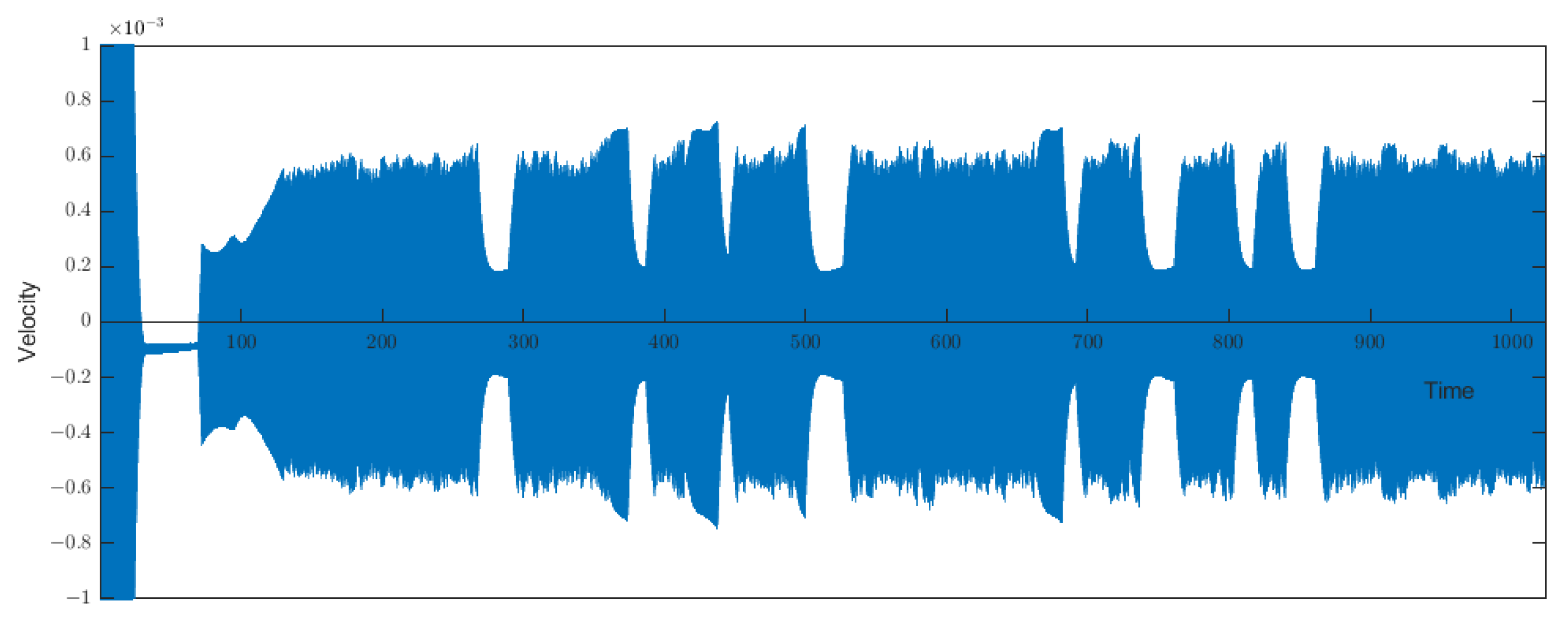
In previous work as [4], using the operator abstract theory, it was proven that if K J = , then the global attractor for system Equation (1) in I R × H ˙ p e r 1 ( 0 , 1 ) × L ˙ p e r 2 ( 0 , 1 ) is reduced to a point.
In this sense, Corollaries 1 and 2 offer the possibility to obtain the same asymptotic behavior for the dynamics with small ϵ, i.e., the attractor is also reduced to a point taking functions f and T a without this condition, that is with K J , but on the finite set K J , this function f and T a satisfy the orthogonality conditions, i.e.,
( 1 b c ) k K J b k c k = 0 .
Next, we also note if the function T a is constant in this case for every f geometry of the loop, we have the set K J = , that is, the global attractor for System Equation (1) in I R × H ˙ p e r 1 ( 0 , 1 ) × L ˙ p e r 2 ( 0 , 1 ) is reduced to a point.
Finally, we note that Proposition 3 implies that when ϵ is sufficiently small and ( 1 b c ) I 1 0 , although there may be small oscillations of the velocity around some fixed value, the sign of the velocity is determined by that of ( 1 b c ) I 1 , and therefore, the fluid motion inside the circuit is always clockwise or always counterclockwise. As in viscoelastic fluids, even with a constant G (see [22]), when we have the orthogonality condition ( 1 b c ) I 1 = 0 , the velocity oscillates around zero, changing sign an infinite number of times, producing complex behavior in the physical device (see Figure 1).

3.3. Fast Solutions in the Case of H = G ϵ ( v ) = G ( v ) ϵ and G ( v ) = g ( R e | v | ) | v |

Hereafter, we consider H = G ϵ ( v ) = G ( v ) ϵ and the friction function G ( v ) = g ( R e | v | ) | v | in order to study the asymptotic behavior of solutions of System (1) for large Reynold’s numbers. Hereafter, we consider H = G ϵ ( v ) = G ( v ) ϵ and the friction function G ( v ) = g ( R e | v | ) | v | in order to study the asymptotic behavior of solutions of System (1) for large Reynold’s numbers.
From the properties of g, it turns out that for nonzero v, G ( v ) | v | if the Reynold’s number is large, but if R e | v | is sufficiently small, then G ( v ) A / R e . Therefore, we cannot expect that the formal limit obtained by setting R e = in (6) (and then G ( v ) = | v | for all v R ) will describe in a faithful manner the dynamics of the system for large R e .
However, we show in this section that it is possible to prove some results about the asymptotic behavior of solutions that retain the velocity bounded away from zero.
First, we considered the stationary solutions with nonzero velocity for large Reynold’s numbers. According to Velázquez (1994), taking G ( v ) = | v | in (11), we obtain the class of stationary solutions denoted by fast stationary solutions.
Note that the set of equilibria with nonzero velocity, ( v f , a k f , d k f ) fast stationary solutions, with R e , i.e., with G ( v ) = | v | , are given by:
a k f = G ( v ) b k G ( v ) + ϵ 2 π k i v = b k 1 ± 2 π k ϵ i w i t h G ( v ) = | v |
d k f = 4 b π 2 k 2 a k 2 π k i v + 4 c π 2 k 2 = b c 2 π k 2 π k + i v f c a k f w i t h a k f = b k 1 ± 2 π k ϵ i
G ( v f ) v f = k K J ( a k f d k f ) c k = I ± w i t h G ( v ) = | v |
plus the compatibility conditions s i g ( I ± ) = ± , where ± denotes the sign of v f .
In these cases, if s i g ( I + ) = + , then ( v + f , a k f , d k f ) , k K J is the positive fast stationary solution, and if s i g ( I ) = , then ( v f , a k f , d k f ) , k K J is the negative fast stationary solution.
Now, we study the existence of fast time-dependent solutions, that is the solutions depending on time, such that the velocity does not go to zero when the time goes to , for large Reynold’s numbers.
Now, we assumed that ( 1 b c ) I 1 0 with I 1 = k K J b k c k as in the above section, and we considered the solutions of System (6) such that lim inf t | v ( t ) | is bounded away from zero as R e , i.e., the sign of v ( t ) is fixed for t large enough. This kind of solutions is called a positive fast time solution if v ( t ) > 0 or a negative fast time solution if v ( t ) < 0 for t and R e large enough.
We show below that the fast stationary solutions such that I ± = ( 1 b c ) k K J b k c k attract the dynamics of fast time-dependent solutions.
Proposition 4.
We assumed there exists a solution of (6) such that v ( t ) is bounded away from zero for t > t 0 > 0 , and thus, the sign of v ( t ) is constant for large enough t.Then, for every k we have:
 (i) 
lim sup t | a k ( t ) a k f | ϵ 2 π | k | | b k | lim sup t | | v ( t ) | G ( v ) 1 | =
= ϵ 2 π | k | | b k | lim sup t | 1 g ( R e | v ( t ) | ) 1 | ;
 (ii) 
lim sup t | d k ( t ) b c a k f | ϵ 2 π | k | | b k | b c lim sup t | | v ( t ) | G ( v ) 1 | =
= ϵ 2 π | k | b c | b k | lim sup t | 1 g ( R e | v ( t ) | ) 1 |
with a k f given by (21), and we also have:
lim sup t | d k ( t ) b c a k f 2 π k π k + i v ( t ) c | ϵ 2 π | k | | b k | b c lim sup t | | v ( t ) | G ( v ) 1 | =
= ϵ 2 π | k | b c | b k | lim sup t | 1 g ( R e | v ( t ) | ) 1 |
Moreover, we have that:
 (iii) 
lim sup t | d k ( t ) d k f | ϵ 2 π | k | | b k | b c lim sup t | | v ( t ) | G ( v ) 1 | + 2 π | k | | d k f | lim sup t | v ( t ) v f | =
= ϵ 2 π | k | b c | b k | lim sup t | 1 g ( R e | v ( t ) | ) 1 | + 2 π | k | | d k f | lim sup t | v ( t ) v f |
with a k f and d k f given by (21) and (22), respectively, as well as with G ( v ) = g ( R e | v | ) | v | .
Proof. (i) We note that:
a k ( t ) = a k ( t 0 ) e [ t 0 t 2 π k i v + G ϵ ( v ) ] + b k t 0 t G ϵ ( v ) e [ s t 2 π k i v + G ϵ ( v ) ] ,
with:
a ^ k ± ( t ) = b k t 0 t G ϵ ( v ) e s t [ G ϵ ( v ) ± 2 π k i G ] d s .
Changing variables r = s t G ϵ , we obtain:
a ^ k ± ( t ) = b k 0 t 0 t G ϵ e ( 1 ± 2 π k i ϵ ) r d r = b k 1 ± 2 π k i ϵ ( 1 e ( 1 ± 2 π k i ϵ ) 0 t G ϵ ) a n d
a ^ k ± ( t ) b k 1 ± 2 π k i ϵ = a k f ( g i v e n   b y   ( 21 ) )   a s t .
Let now τ k ± ( t ) = a k ( t ) a ^ k ± ( t ) ; from (28), we have:
lim sup t | τ k ± ( t ) | | b k | lim sup t t 0 t G ϵ e s t G ϵ | e s t 2 π k i v e s t ± 2 π k i G | d s .
Using now that | e s t 2 π k i ( v G ) 1 | 2 π | k | s t | v G | , we have that:
lim sup t | τ k ± ( t ) | 2 π | k | | b k | lim sup t t 0 t G ϵ e s t G ϵ s t | v G | d s .
Next, using again L’Hôpital’s lemma, we obtain:
lim sup t t 0 t G ϵ e s t G ϵ s t | v G | d s =
= lim sup t t 0 t G ϵ e t 0 s G ϵ ( t 0 t | v G | d s t 0 s | v G | d s ) e t 0 t G ϵ
lim sup t | v G | t 0 t G ϵ e t 0 s G ϵ G ϵ e t 0 t G ϵ lim sup t | v G | G ϵ ϵ lim sup t | ± v G 1 | ,
since:
lim sup t t 0 t G ϵ e t 0 s G ϵ e t 0 t G ϵ 1 .
Thus, we obtain:
lim sup t | τ k ± ( t ) | ϵ 2 π | k | | b k | lim sup t | | v | G ( v ) 1 |
and we conclude (i);
(ii) Next, we note that:
d k ( t ) = d k ( t 0 ) e 4 c π 2 k 2 t e t 0 t 2 π k i v + 4 b π 2 k 2 t 0 t a k ( s ) e 4 c π 2 k 2 ( t s ) e s t 2 π k v i ,
and if we denote by:
d ^ k ( t ) = 4 b π 2 k 2 a k f t 0 t e [ s t 2 π k v i + 4 c π 2 k 2 ] d s = 4 b π 2 k 2 a k f t 0 t e t 0 s [ 2 π k v i + 4 c π 2 k 2 ] d s e t 0 t [ 2 π k v i + 4 c π 2 k 2 ] d s ;
then working as before and applying L’Hôpital’s lemma, we have that:
lim inf t d ^ k ( t ) lim sup t d ^ k ( t ) b c a k f lim sup t 2 π k 2 π k + i v c b c a k f ,
since:
lim sup t t 0 t e t 0 s 2 π k v i + 4 c π 2 k 2 e t 0 t 2 π k v i + 4 c π 2 k 2 lim sup t 1 2 π k v i + 4 c π 2 k 2 .
Moreover, we also obtain:
lim sup t | d k ( t ) d ^ k ( t ) | lim sup t 4 b π 2 k 2 | 2 π k v i + 4 c π 2 k 2 | lim sup t | a k ( t ) a k f |
with 4 π 2 k 2 | 2 π k v c i + 4 π 2 k 2 | 1 , that is:
lim sup t | d k ( t ) d ^ k ( t ) | b c lim sup t | a k ( t ) a k f | ,
and we conclude (ii).
Finally, we note that:
d k ( t ) = 4 b π 2 k 2 a k f t 0 t e [ [ 2 π k v f i + 4 c π 2 k 2 ] ( t s ) d s d k f ( g i v e n b y ( 22 ) ) a s t
and:
d k ( t ) d k ( t ) = d k ( t 0 ) e 4 c π 2 k 2 t e t 0 t 2 π k i v + 4 b π 2 k 2 ( l 1 ( t ) + l 2 ( t ) )
with:
l 1 ( t ) = t 0 t ( a k ( s ) a k f ) e 4 c π 2 k 2 ( t s ) e s t 2 π k v i ,
l 2 ( t ) = a k f t 0 t e ( 4 c π 2 k 2 + 2 π k i v f ) ( t s ) e s t 2 π k i ( v v f ) 1 )   w h e r e
| e s t 2 π k i ( v v f ) 1 ) | 2 π | k | s t | v v f | ; and proceeding as before and applying L’Hôpital’s lemma, we obtain:
4 b π 2 k 2 lim sup t l 1 ( t ) b c lim sup t | a k ( t ) a k f | a n d
lim sup t l 2 ( t ) 2 π | k | a k f lim sup t t 0 t e α k s t 0 t | v v f | t 0 s | v v f | e α k t
2 π | k | a k f α k lim sup t | v ( t ) v f |
with α k = 4 c π 2 k 2 + 2 π k i v f ; we conclude. □
Note that, from the above subsection that we can take ϵ 0 small enough such that lim inf t | v ( t ) | > 0 , and then, R e | v ( t ) | as R e . Now, we considered g ( s ) 1 + B s m + o ( s m ) as s (an assumption that was made in Velázquez, 1994), and then, with m = 1 and s = R e | v ( t ) | , we obtain | 1 g ( R e | v ( t ) | ) 1 | B ( 1 R e ) 1 | v ( t ) | = B ( 1 R e ) δ ( t ) w i t h lim sup t B ( 1 R e ) δ ( t ) B ( 1 R e ) = o ( 1 ) a s R e .
Now, we can prove the following corollary, which precisely states that the dynamics of fast time-dependent solutions is attracted towards fast stationary solutions.
Corollary 3.
Under the above notations and hypotheses, we can prove that as R e , there exists a positive fast time-dependent solution such that if s i g n ( I + ) = + with I + = ( 1 b c ) k K J b k c k , then:
lim sup t | a k ( t ) a k f | = lim sup t | a k ( t ) b k 1 + ϵ 2 π k i | B ( 1 R e ) = o ( 1 ) ,
lim sup t | d k ( t ) b c a k f | b c B ( 1 R e ) = o ( 1 )
lim sup t | d k ( t ) d k f | = lim sup t | d k ( t ) b c 2 π k 2 π k v f c i a k | D ( 1 R e ) = o ( 1 )
lim sup t | v ( t ) v + f | E ( 1 R e ) = o ( 1 ) a s R e .
where v + f is the solution of | v | v = I + and B , D , E are positive constants independent of R e . On the other hand, is s i g n ( I + ) = , so no fast time-dependent solutions exist.
The same holds for negative fast time-dependent solutions by changing + to −.
Proof. 
From Proposition 4, we can take ϵ 0 small enough such that | v ( t ) | 0 for t large enough, and we have that:
lim sup t | a k ( t ) a k f | = o ( 1 ) a n d lim sup t | d k ( t ) b c a k f | = o ( 1 ) a s R e .
Now, let I 2 ( t ) = k K J ( a k ( t ) a k f ) c k and I 3 ( t ) = k K J ( d k ( t ) b c a k f ) c k , so there exits a positive constant F independent of R e , such that:
lim sup t ( | I 2 ( t ) I 3 ( t ) | ) = F ( 1 R e ) a n d lim sup t ( | I 2 ( t ) | + | I 3 ( t ) | ) = F ( 1 R e )
with F ( 1 R e ) = o ( 1 R e ) = o ( 1 ) a s R e .
Next, we considered the equations for the velocity v ( t ) :
ϵ d v d t + G ( v ) v = k K J ( a k ( t ) d k ( t ) ) c k = I 2 ( t ) I 3 ( t ) + ( 1 b c ) k K J a k f c k
and taking into account that a k f b k as ϵ 0 , given δ > 0 , there exists ϵ 0 such that ( 1 b c ) k K J a k f c k ( 1 b c ) k K J b k f c k + δ , and we note that the stationary velocity v + f satisfies that:
| v + f | v + f = k K J ( a k f d k f ) c k = ( 1 b c ) k K J b k f c k .
That is
ϵ d v d t + G ( v ) v | v + f | v + f = I 2 ( t ) I 3 ( t ) + δ = δ 1 ( t ) + δ   a n d   lim sup t | δ 1 ( t ) | = o ( 1 ) + δ   a s   R e . Furthermore, it is important to note that δ 2 ( t ) = G ( v ) v | v | v satisfies that lim sup t ( G ( v ) v | v | v ) = o ( 1 ) since if R e , then G ( v ) | v | . Then, read the equations for v as:
ϵ d ( v v + f ) d t + | v | v | v + f | v + f δ 1 ( t ) δ 2 ( t ) + δ = δ ( t ) + δ ,
with lim sup t δ ( t ) = o ( 1 )   a s   R e , that is δ ( t ) = o ( 1 ) for large enough t. If we multiply by ( v v + f ) and use the function | s | s , which monotonically increasing, working as the above section, from Gronwall’s lemma, we obtain lim sup t | v v + f | o ( 1 ) as R e .
Finally, using this together with (27), we also obtain lim sup t | d k ( t ) d k f | 0 ( 1 ) as R e , and we conclude. □
Remark 2.
Note that for a thermosyphon model where the fluid has only one component (see [15]), the condition s i g ( I + ) = + implies the existence of a unique positive fast stationary solution, which is moreover stable.
Therefore, fast time-dependent solutions must exist in its basin of attraction. The corollary above states then that all positive fast time-dependent solutions must be close enough to the stationary one. The same remark applies for negative fast solutions.
On the other hand, the corollary contains a criterion for the nonexistence of fast time-dependent solutions. Furthermore, note that the velocity for all other solutions must change sign an infinite number of times.

4. Numerical Results

In this section, we analyze several numerical experiments in order to illustrate the theoretical results. In particular, these experiments show the asymptotic behavior of the dynamics of fast time-dependent solutions for large Reynold’s numbers.
We solved the system of ordinary differential equations (6) using the solvers of MATLAB for stiffness equations. Our experiments were performed using ODE15s with a local error tolerance of 10 9 except for the first one (see Figure 1), where we considered a local error tolerance of 10 10 . Moreover, except the case where b = c , we could obtain very similar results using the ODE45 solver. The simulations were performed in double precision with machine epsilon ϵ M 2.2 × 10 16 .
We plot some interesting situations that reflect in a good way the previous results. As the system is multidimensional, we present the results in temporal graphs (a given variable versus time) and phase space graphs (two physical variables plotted against each other).
Throughout this section, we consider the friction law represented by G of the form G ( v ) = | v | + A G R e . Note that G ( v ) | v | if R e goes to infinity.
Note that we deal with the positive fast stationary solutions. Since we considered a circular geometry, we have J = { ± 1 } and K J = { ± 1 } . Then, we took k = 1 and omitted the equation for k , the conjugate of k. Therefore, from (21)–(23), we have the following system of equations:
a 1 f = b 1 1 + 2 π ϵ i
d 1 f = b c 2 π i 2 π + i v f c a 1 f
( v f ) 2 = 2 ( a 1 f c 1 ) 2 ( d 1 f c 1 )
where the unknowns are a 1 f , the Fourier mode of the temperature, d 1 f , the Fourier mode of the solute concentration, and v f , the velocity of the fluid.
In order to reduce the number of free parameters, we made a change to variables a 1 c 1 a 1 y d 1 c 1 d 1 , and we denote the real and imaginary part of b 1 c 1 by A + B i . For the Soret effect diffusion coefficients b and c, we assumed the values calculated by Hart in [1], which consider a thermosyphon of circular geometry of radius R 0 (for the loop) and R p (for the pipe). Hart took the values for a mixture of alcohol and water, borrowed from Hurle and Jakeman [7]. This reference settles down that c = D s V R 0 is the number of Lewis, where D s is the diffusivity of the solute that has a value for such a mixture of 10 5 cm 2 s 1 and V is the scale of the velocity, with a value of 10 2 cms 1 for a circular thermosyphon whose loop-to-pipe-radius ratio is 10. Therefore, we took c = 10 3 . Moreover, as Hart indicated in [1], b (Soret diffusion coefficient) is a parameter that determines the qualitative behavior of the variable. Finally, A and B refer in this model to the position-dependent ( x ) heat flux inside the loop.
Then, since we want to guarantee that:
s i g n ( I + ) = + with I + = ( 1 b c ) k ± 1 b k c k ,
we took b = 10 4 and A = B = 30 . In fact, taking A = 0 , B = 30 and c = b = 10 2 , we obtained a velocity oscillating close to zero. Therefore, according to Proposition 3, we cannot guarantee that the velocity keeps the same sign; see Figure 1. This example reflects very well how, even for a small epsilon, there may be solutions for which the velocity changes sign an infinite number of times and whose dynamics may be very involved. This produces complex behavior in the physical device.
First of all, we kept fixed ϵ = 10 2 , and we varied the Reynold’s number in order to analyze the asymptotic behavior of the solutions of (6). For this particular case, the fast stationary solution is given by:
a 1 f = 31.7595738203323 + 28.004487124098 i d 1 f = 0.002209826274535 0.00250215970862028 i v f = 7.9696127878408
The numerical experiments were carried out for R e = 10 to R e = 10 5 , and we took as initial values the following ones:
a 0 = 25 + 20 i , d 0 = 0.02 0.002 i v 0 = 9 .
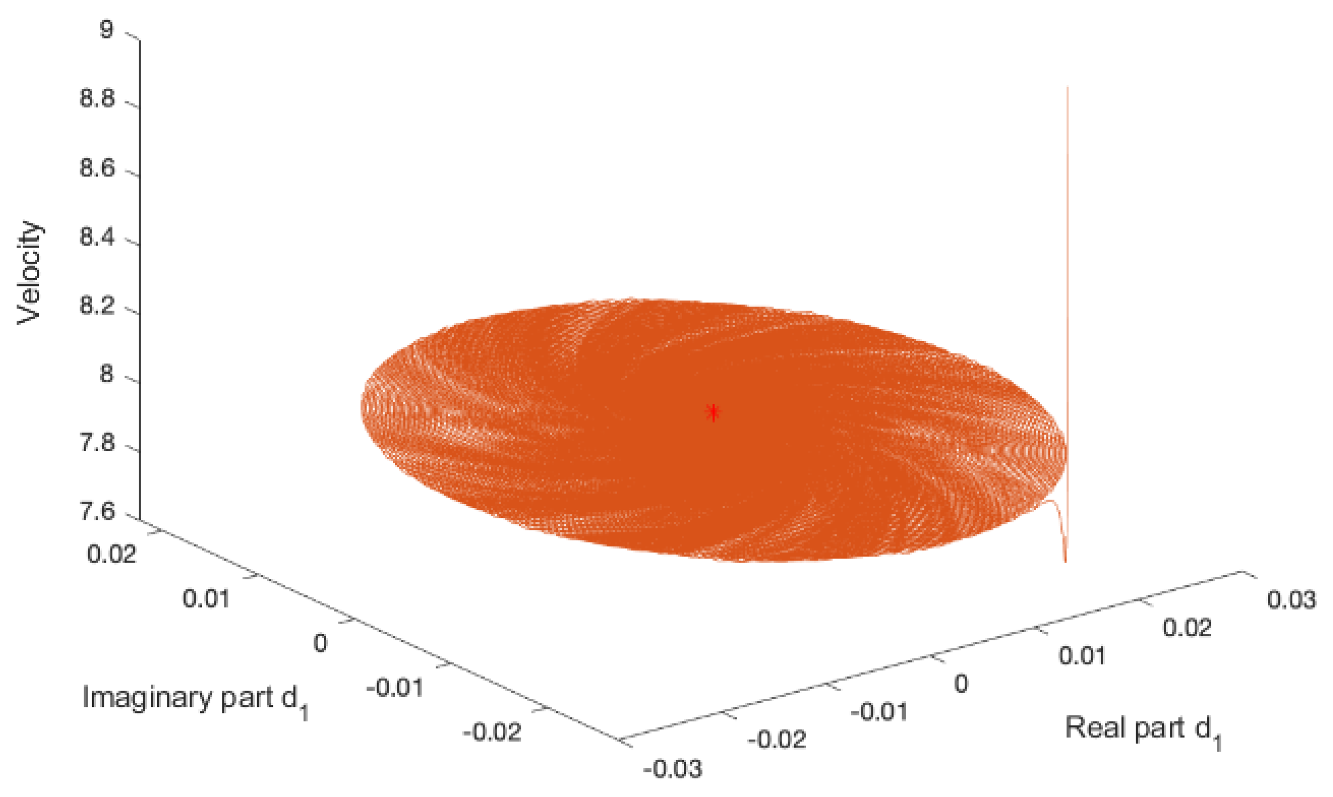
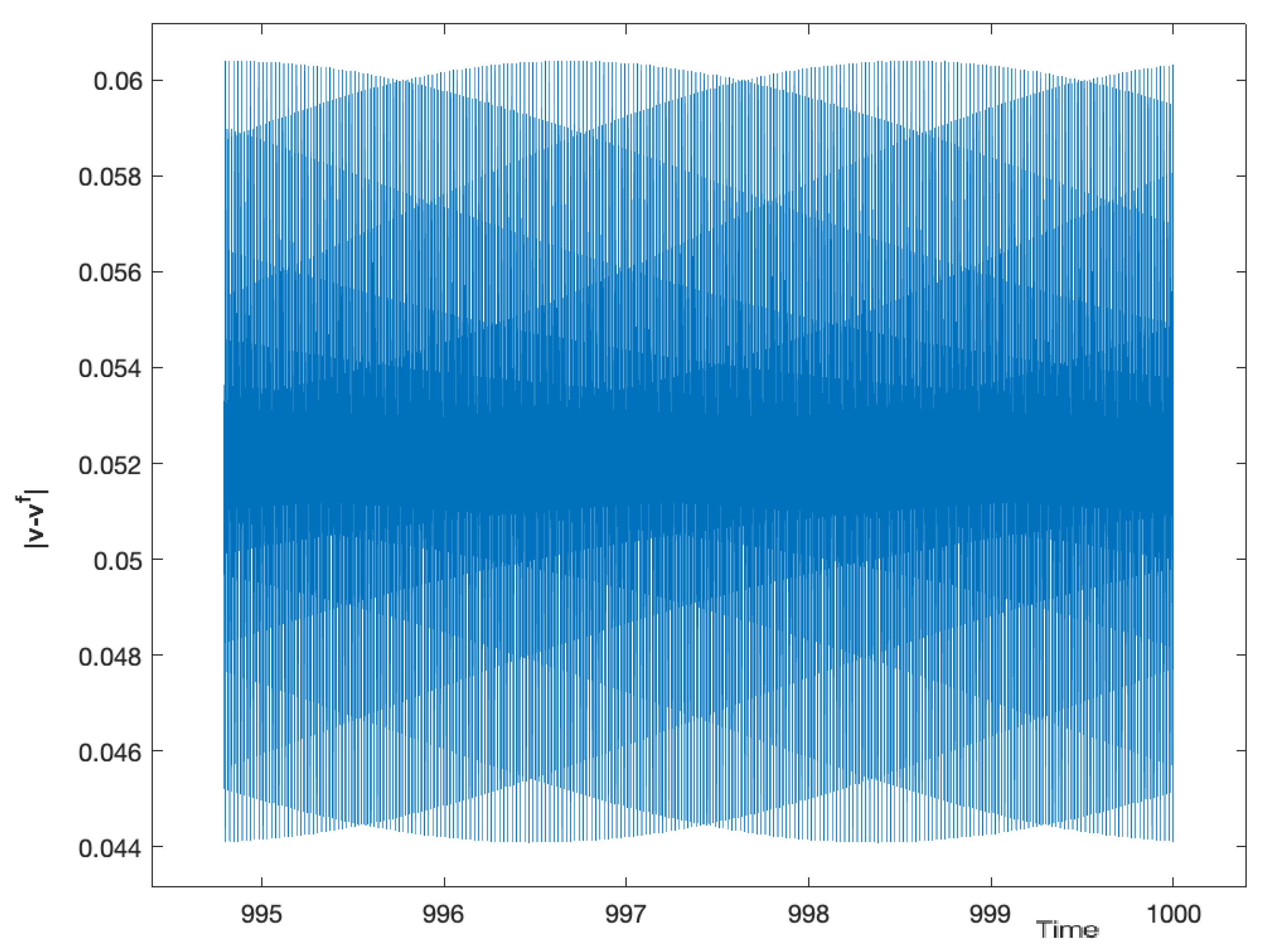
We show that the dynamics of fast time-dependent solutions are attracted towards fast stationary solutions. After some more or less complicated transitions, fast time-dependent solutions are close to the stationary one; see Figure 2, Figure 3 and Figure 4 Note that although there are small oscillations of the velocity, it maintains a constant sign for a large time, and therefore, the fluid undergoes a sustained motion.
Moreover, we observed that if R e is increasing, then the fast time-dependent solutions are closer to the fast stationary solution considering the same time; see Figure 5 and Figure 6.
Note that the numerical results were in good agreement with the estimates obtained in Corollary 3. For instance, if R e = 10 4 from the numerical results, we obtain | v v f | < 10 5 .
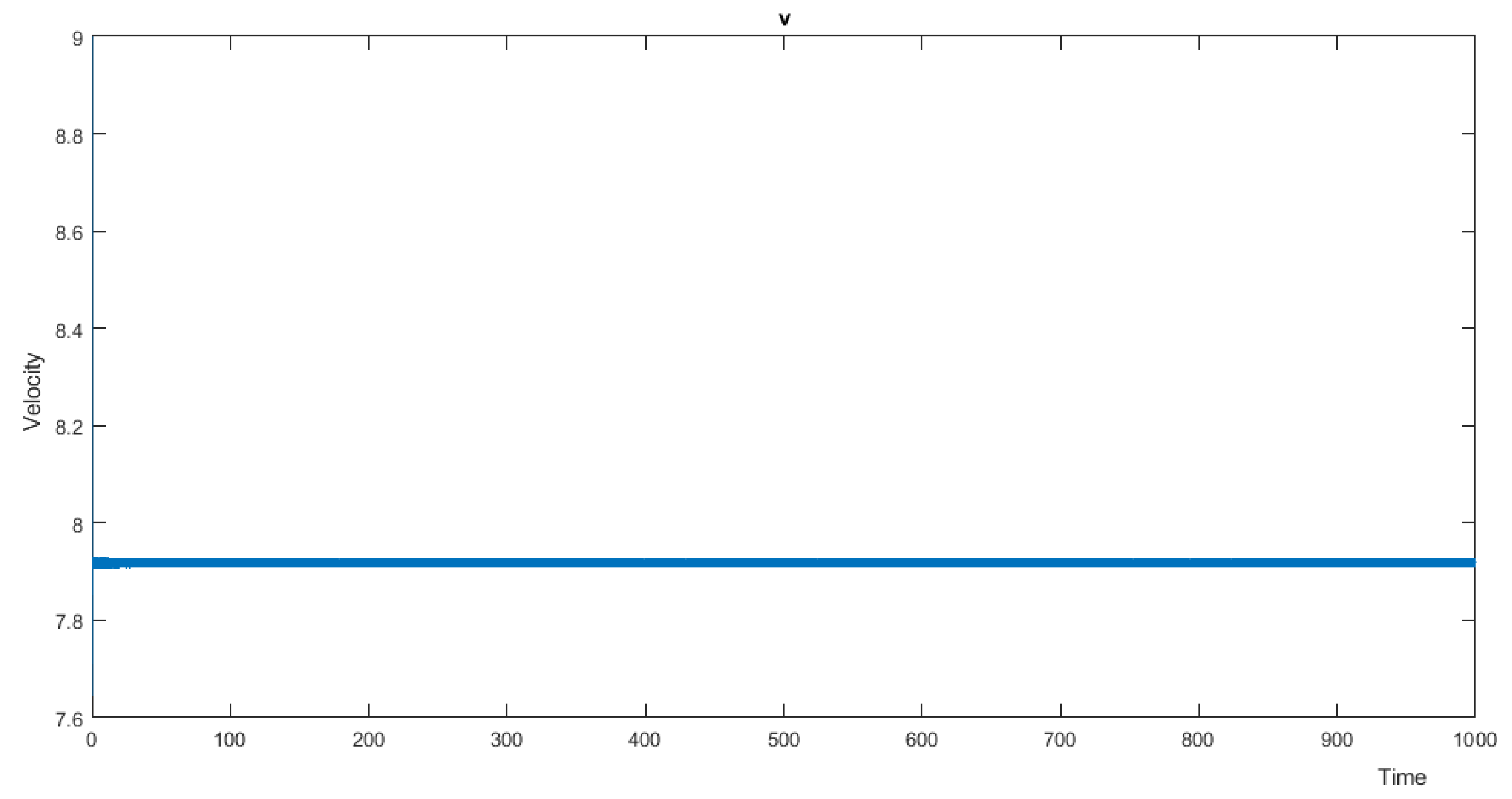
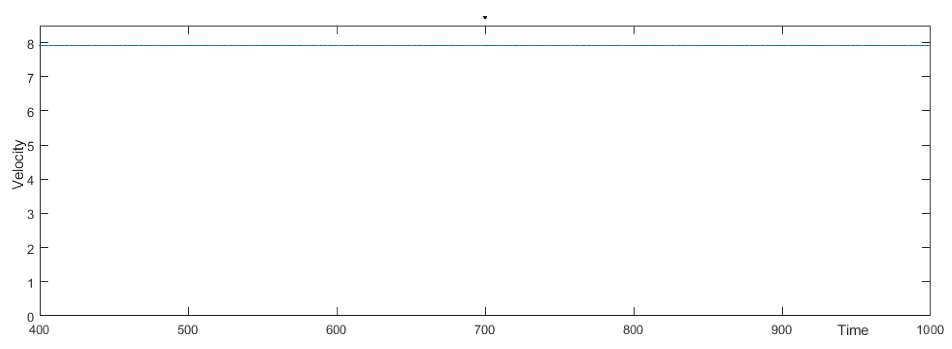
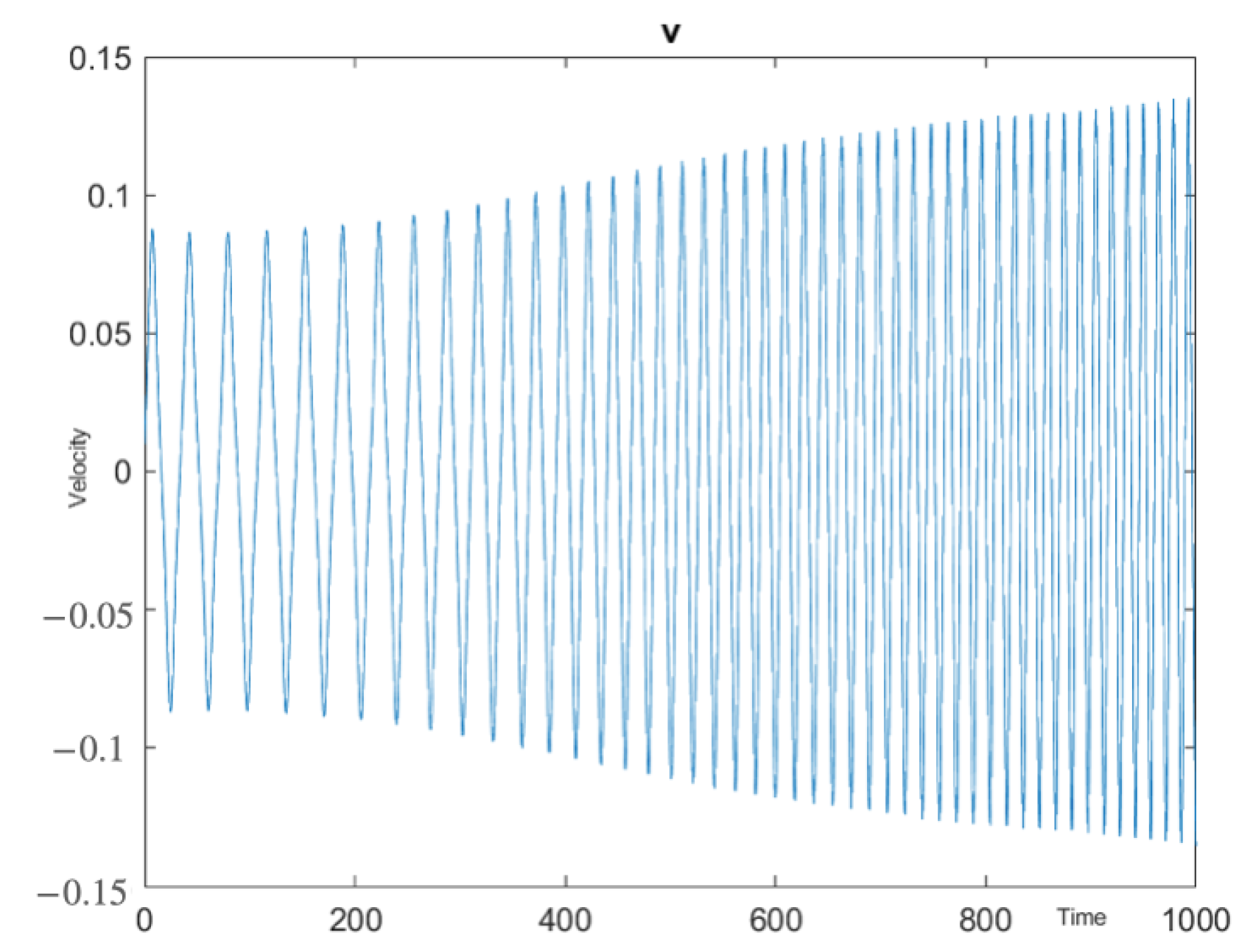
Note that these numerical experiments show the important fact that, as we stated in previous sections, for some values of the parameters, a fast time-dependent solution must exist in the basin of attraction of the fast stationary solution. This is very relevant from a practical point of view because it allows us to distinguish in which situations the device with a binary fluid works effectively, and velocity is not oscillating around zero, or by contrast, it presents complicated regimes where irregular or chaotic behaviors appear. In this sense, we would like to highlight the importance of taking ϵ small enough. Observe that for ϵ = 10 2 and R e = 10 , the velocity of the system tends to v f , even considering an initial velocity close to zero; see Figure 7. However, increasing ϵ , the behavior of the velocity becomes involved. For instance, for ϵ = 10 3 (see Figure 8), we illustrate a scenario where the velocity does not stabilize and it is oscillating around zero.

5. Conclusions

The aim of this work was to obtain a criterion about the existence and asymptotic behavior of fast solutions for this thermosyphon model as R e tends to . Notice that determining conditions in which the thermosyphon functions effectively or, by contrast, knowing when it presents chaotic behaviors is of great interest from a practical point of view.
In this respect, we obtained the following results:
  • If ( 1 b c ) k K J b k c k 0 , then no solutions satisfies l i m i t t v ( t ) = 0 ;
  • Let ( v + f , a k f , d k f ) be a positive fast stationary solutions, i.e., v + f | v + f | = ( 1 b c ) k K J b k c k > 0 , and ϵ small enough such that lim i n f t | v ( t ) | > 0 , i.e., the sign of v ( t ) is constant for large enough t. Then, Corollary 3 precisely states in which conditions the fast stationary solution attracts the dynamics of fast time-dependent solutions. In particular, we proved the following:
    (i)
    If v ( t ) > 0 for large enough t, there exists a positive fast time-dependent solution ( v ( t ) , a k ( t ) , d k ( t ) ) as R e , i.e.,:
    lim sup t | a k ( t ) a k f | B ( 1 R e ) = o ( 1 ) a s R e .
    lim sup t | d k ( t ) d k f | D ( 1 R e ) = o ( 1 ) a s R e .
    lim sup t | v ( t ) v + f | E ( 1 R e ) = o ( 1 ) a s R e .
    B , D , E are positive constants independent of R e ;
    (ii)
    If, v ( t ) < 0 for large enough t, no fast time-dependent solutions exist;
  • The same holds for negative fast time-dependent solutions by changing + to −;
  • We showed numerically that the characterization of the existence of fast time-dependent solution that is attracted to the fast stationary one works. In particular, we gave examples where fast solutions exists, and we also chose other values of the parameters where the velocity changes sign an infinite number of times without preserving the sign for a large time.

Author Contributions

Methodology, Á.J.-C.; software, M.V.-P.; formal analysis, Á.J.-C.; investigation, Á.J.-C. and M.V.-P.; writing—original draft preparation, Á.J.-C. and M.V.-P.; writing—review and editing, Á.J.-C. and M.V.-P.; funding acquisition, Á.J.-C. and M.V.-P. All authors have read and agreed to the published version of the manuscript.

Funding

This research was partially supported by Grants PID2019-106339GB-I00 funded by MCIN/AEI/10.13039/501100011033, Spain, and PID2019-103860GB-I00 funded by MCIN/AEI/Spain; by GR58/08 Grupo 920894 BSCH-UCM from Grupo de Investigación CADEDIF and Grupo de Dinámica No Lineal (U.P. Comillas) Spain.

Institutional Review Board Statement

Not applicable.

Informed Consent Statement

Not applicable.

Data Availability Statement

Not applicable.

Conflicts of Interest

The authors declare no conflict of interest.

Appendix A. Global Existence and Asymptotic Behavior for a Large Time

We rewrite here the results about the well-posedness of the existence of the global attractor and the inertial manifold for the solutions of our model; for the proof, see Theorems 3.3, 4.1, and 4.2 together with Corollary 4.1 in [4].
Proposition A1.
Under the above notation, we suppose that r G ( r ) is locally Lipschitz, H C 1 , with G ( s ) G 0 > 0 , H ( s ) H 0 > 0 , T a H ˙ p e r 2 ( 0 , 1 ) , f L ˙ p e r 2 ( 0 , 1 ) given by (2), the initial data T 0 H ˙ p e r 2 ( 0 , 1 ) given by T 0 ( x ) = k I Z a k 0 e 2 π k i x , and S 0 L ˙ p e r 2 ( 0 , 1 ) given by S 0 ( x ) = k I Z d k 0 e 2 π k i x . Recalling the expansions:
T a ( x ) = k I Z b k e 2 π k i x   a n d   f ( x ) = k I Z c k e 2 π k i x   w i t h   I Z = I Z { 0 }
T ( t , x ) = k I Z a k ( t ) e 2 π k i x   a n d   S ( t , x ) = k I Z d k ( t ) e 2 π k i x
then the global solution ( v , T , S ) of the system (1) satisfies the following:
(i)
ϵ d v d t + G ( v ) v = k I Z ( a k ( t ) d k ( t ) ) c ¯ k
where the coefficients a k ( t ) and d k ( t ) satisfy the equations:
d ( a k ) d t + 2 k π v i + H ( v ) a k ( t ) = H ( v ) b k , a k ( 0 ) = a k 0 , k I Z d ( d k ) d t + 2 k π v i + 4 c k 2 π 2 d k ( t ) = 4 b π 2 k 2 a k ( t ) , d k ( 0 ) = d k 0 , k I Z .
(ii)There exists a compact and connected global attractor A in I R × H ˙ p e r 2 ( 0 , 1 ) × L ˙ p e r 2 ( 0 , 1 ) for the flow of the system (1). In particular, if T a H ˙ p e r m ( 0 , 1 ) with m 2 , we have that the global attractor A I R × H ˙ p e r m ( 0 , 1 ) × H ˙ p e r m ( 0 , 1 ) and is compact in this space;
(iii)Inertial manifold associated with T a :
We have that there exists an inertial manifold M (see the definition in References [23,24,25]) for the semigroup S ( t ) in the phase space Y = I R × H ˙ p e r m ( 0 , 1 ) × H ˙ p e r m 2 ( 0 , 1 ) , i.e., a submanifold of Y such that:
  • S ( t ) M M for every t 0 , with A M ;
  • There exists δ > 0 satisfying that for every bounded set B Y , there exists C ( B ) 0 such that d i s t ( S ( t ) , M ) C ( B ) e δ t , t 0 (see, for example, [23,24,25]).
Assume that T a H ˙ p e r m ( 0 , 1 ) and f L ˙ p e r 2 ( 0 , 1 ) , with:
T a = k K b k e 2 π k i x
where b k 0 for every k K I Z with 0 K , since T a ( x ) d x = 0 . We denote by V m the closure of the subspace of H ˙ p e r m ( 0 , 1 ) generated by { e 2 π k i x , k K } .
Then, the set M = I R × V m × V m 2 is an inertial manifold for the flow of S ( t ) ( v 0 , T 0 , S 0 ) = ( v ( t ) , T ( t ) , S ( t ) ) in the space Y = I R × H ˙ p e r m ( 0 , 1 ) × H ˙ p e r m ( 0 , 1 ) . Moreover, if K is a finite set, the dimension of M is 2 | K | + 1 , where | K | is the number of elements in K, and the flow on M is given by:
ϵ d v d t + G ( v ) v = k K ( a k ( t ) d k ( t ) ) c ¯ k d ( a k ) d t + 2 k π v i + H ( v ) a k ( t ) = H ( v ) b k , k K , d ( d k ) d t + 2 k π v i + 4 c k 2 π 2 d k ( t ) = 4 b π 2 k 2 a k ( t ) , k K , a k = d k = 0 , k K ;
(iv)The reduced system of ODE’s with the relevant Modes k K J (involving T a and f ):
Moreover, if we suppose that f L ˙ p e r 2 ( 0 , 1 ) is given by:
f ( x ) = k J c k e 2 π k i x ,
where J = k I Z / c k 0 , I Z = I Z 0 , since f ( x ) d x = 0 , then, on the inertial manifold, we have ( T S ) f = k K ( a k ( t ) d k ( t ) ) c k = k J ( a k ( t ) d k ( t ) ) c k , and regarding the right-hand side of the first equation of (A2), we can observe that the velocity of the fluid is independent of the coefficients for temperature a k ( t ) , d k ( t ) for every k I Z ( K J ) .
Note that in (A2), the set of equations for a k ( t ) , d k ( t ) with k K J (therelevant modes), together with the equation for v are a subsystem of coupled equations, which describe the dynamics of the original system.
Moreover, the equations for a k , d k are conjugates of the equations for a k ( t ) , d k ( t ) ; therefore, s u m k K 5 J a k ( t ) c k = 2 R e a l ( s u m k ( K J ) + a k ( t ) c k ) , and analogously, s u m k K J d k ( t ) c k = 2 R e a l ( s u m k ( K J ) + d k ( t ) c k ) .
We note that 0 K J , and since K = K and J = J , then the set K J has an even number of elements, which we denote by 2 n 0 . Therefore, the number of elements in the set of positive elements of i n   K J , ( K J ) + is n 0 .
Therefore, the asymptotic behavior of the system is described by a system of N = 4 n 0 + 1 coupled equations in I R N , which determine ( v , a k , d k ) , k K J .
After solving this, we must solve the equations for k K J , which are linear autonomous equations.
Finally, we note that to obtain the estimates of the velocity, we made use of the following version of L’Hôpital’s lemma; see [16] for the details.
Lemma A1.
L’Hôpital’s Lemma. Assume f and g are real differentiable functions on ( a , b ) , b , g ( x ) 0 on ( a , b ) , and lim x b g ( x ) = :
(i) If lim sup x b f ( x ) g ( x ) = L , then lim sup x b f ( x ) g ( x ) L ;
(ii) If lim inf x b f ( x ) g ( x ) = L , then lim inf x b f ( x ) g ( x ) L .

References

  1. Hart, J.E. A Model of Flow in a Closed-Loop Thermosyphon including the Soret Effect. J. Heat Transf. 1985, 107, 840–849. [Google Scholar] [CrossRef]
  2. Hollinger, S.; Lucke, M. Influence of the Soret effect on convection of binary fluids. Phys. Rev. E 1998, 57, 4238–4249. [Google Scholar] [CrossRef] [Green Version]
  3. Herrero, M.A.; Velazquez, J.J.-L. Stability analysis of a closed thermosyphon. Eur. J. Appl. Math. 1990, 1, 1–24. [Google Scholar] [CrossRef]
  4. Jiménez-Casas, A.; Rodríguez-Bernal, A. Finite-dimensional asymptotic behavior in a thermosyphon including the Soret effect. Math. Meth. Appl. Sci. 1999, 22, 117–137. [Google Scholar] [CrossRef]
  5. Casas, A.J.; Rodríguez-Bernal, A. Dinámica No Lineal: Modelos de Campo de Fase y un Termosifón Cerrado; Editorial Académica Española; Lap Lambert Academic Publishing GmbH and Co. KG: Saarbrücken, Germany, 2012. [Google Scholar]
  6. Jiménez-Casas, A.; Castro, M. A Thermosyphon model with a viscoelastic binary fluid. Electron. J. Differ. Equ. 2016, 1072–6691. [Google Scholar]
  7. Hurle, D.T.J.; Jakerman, E. Soret-Driven Thermosolutal Convection. J. Fluid Mech. 1971, 47, 667–687. [Google Scholar] [CrossRef]
  8. Keller, J.B. Periodic oscillations in a model of thermal convection. J. Fluid Mech. 1966, 26, 599–606. [Google Scholar] [CrossRef]
  9. Ding, L.; Wang, W.; Li, B. Numerical Simulation of a Thermosyphon Radiator Used in Electronic Devices. J. Robot. Mech. Eng. 2021, 1, 1–6. [Google Scholar] [CrossRef]
  10. Czerwiński, G.; Wołoszyn, J. Numerical Study of a Cooling System Using Phase Change of a Refrigerant in a Thermosyphon. Energies 2021, 14, 3634. [Google Scholar] [CrossRef]
  11. Jasim, A.K.; Freegah, B.; Alhamdo, M.H. Numerical and experimental study of a thermosyphon closed-loop system for domestic applications. Heat Transf. 2021, 50, 292–312. [Google Scholar] [CrossRef]
  12. Asogwa, K.K.; Mebarek-Oudina, F.; Animasaun, I.L. Comparative Investigation of Water-Based Al2O3 Nanoparticles Through Water-Based CuO Nanoparticles Over an Exponentially Accelerated Radiative Riga Plate Surface via Heat Transport. Arab. J. Sci. Eng. 2022, 47, 1–18. [Google Scholar] [CrossRef]
  13. Djebali, R.; Mebarek-Oudina, F.; Rajashekhar, C. Similarity solution analysis of dynamic and thermal boundary layers: Further formulation along a vertical flat plate. Phys. Scr. 2021, 96, 085206. [Google Scholar] [CrossRef]
  14. Warke, A.S.; Ramesh, K.; Mebarek-Oudina, F.; Abidi, A. Numerical investigation of the stagnation point flow of radiative magnetomicropolar liquid past a heated porous stretching sheet. J. Therm. Anal. Calorim. 2021, 147, 1–12. [Google Scholar] [CrossRef]
  15. Velázquez, J.J.L. On the dynamics of a closed thermosyphon. SIAM J. Appl. Math. 1994, 54, 1561–1593. [Google Scholar] [CrossRef] [Green Version]
  16. Rodríguez-Bernal, A.; Van Vleck, E.S. Complex oscillations in a closed thermosyphon. Int. J. Bif. Chaos 1998, 8, 41–56. [Google Scholar] [CrossRef]
  17. Liñán Martínez, A. Analytical description of chaotic oscillations in a toroidal thermosyphon. In Fluid Physics; Velarde, M.G., Christov, C.I., Eds.; Lecture Notes of Summer Schools; World Scientific: River Edge, NJ, USA, 1994. [Google Scholar]
  18. Debbasch, F.; Rivet, J.P. The Ludwig-Soret effect and stochastic processes. J. Chem. Thermodyn. 2011, 43, 300–306. [Google Scholar] [CrossRef]
  19. Lakshminarayana, P.A.; Murthy, P.V.S.N.; Gorla, R.S.R. Soret-driven thermosolutal convection induced by inclined thermal and solutal gradients in a shallow horizontal layer of a porous medium. J. Fluid Mech. 2008, 612, 1–19. [Google Scholar] [CrossRef]
  20. Welander, P. On the oscillatory instability of a differentially heated fluid loop. J. Fluid Mech. 1967, 29, 17–30. [Google Scholar] [CrossRef]
  21. Jiménez-Casas, A. A coupled ODE/PDE system governing a thermosyphon model. Nonlinear Anal. Theory Methods Appl. 2001, 47, 687–692. [Google Scholar] [CrossRef]
  22. Jiménez-Casas, A. Asymptotic behavior of a closed-loop thermosyphon with linear friction and viscoelastic binary fluid. Math. Meth. Appl. Sci. 2019, 42, 6791–6809. [Google Scholar] [CrossRef]
  23. Foias, C.; Sell, G.R.; Temam, R. Inertial Manifolds for Nonlinear Evolution Equations. J. Diff. Equ. 1985, 73, 309–353. [Google Scholar] [CrossRef] [Green Version]
  24. Rodríguez-Bernal, A. Inertial Manifolds for dissipative semiflows in Banach spaces. Appl. Anal. 1990, 37, 95–141. [Google Scholar] [CrossRef]
  25. Rodríguez-Bernal, A. Attractor and Inertial Manifolds for the Dynamics of a Closed Thermosyphon. J. Math. Anal. Appl. 1995, 193, 942–965. [Google Scholar] [CrossRef] [Green Version]
Figure 1. Example of velocity under the assumption of the orthogonality condition b = c .
Mathematics 10 01098 g001
Figure 2. Concentration–velocity phase diagram ( R e a l   ( d ) , I m   ( d ) , v ) for a Reynold’s number of 10.
Mathematics 10 01098 g002
Figure 3. | v v f | for a Reynold’s number of 10.
Mathematics 10 01098 g003
Figure 4. Velocity evolution for a Reynold’s number of 10.
Mathematics 10 01098 g004
Figure 5. Velocity evolution for a Reynold’s number of 10 4 .
Mathematics 10 01098 g005
Figure 6. | v v f | for a Reynold’s number of 10 4 .
Mathematics 10 01098 g006
Figure 7. v evolution taking v 0 = 0.01 .
Mathematics 10 01098 g007
Figure 8. v evolution taking v 0 = 0.01 .
Mathematics 10 01098 g008
Publisher’s Note: MDPI stays neutral with regard to jurisdictional claims in published maps and institutional affiliations.

