Clustering Based on Continuous Hopfield Network

Abstract

Clustering aims to group n data samples into k clusters. In this paper, we reformulate the clustering problem into an integer optimization problem and propose a recurrent neural network with $n\times k$ neurons to solve it. We prove the stability and convergence of the proposed recurrent neural network theoretically. Moreover, clustering experiments demonstrate that the proposed clustering algorithm based on the recurrent neural network can achieve the better clustering performance than existing clustering algorithms.

1. Introduction

Clustering has been widely studied by machine learning and plays a very important role in various engineering fields. Shaheen et al. [1] presented a new method for clustering, based on the reinforcement factor and the congruence modulo operator. Abdullah et al. [2] utilized k-means to analyze the COVID-19 pandemic. Yeoh et al. [3] proposed a new method that utilizes metaheuristic optimization to improve the performance of the initialization phase.

Clustering aims to group the data points with similar patterns into one cluster. Over the last few decades, relevant scholars have put forward and improved a series of clustering algorithms [4,5,6,7,8,9,10,11,12]. The representative of clustering algorithms is the k-means, which can discover the latent data structure and achieve clustering via the structure. Spectral clustering (SC) [4,5,10] constructs an affinity graph to model the geometrical information within data, and the clustering results respect the graph structure. Some extensions of SC methods [6,7,8] have been proposed to model the nonlinear geometrical structure of data. In addition, the projected clustering algorithm [9] was mentioned, aiming to think over the local information and the global structure of data. Some researchers have improved some clustering to enhance clustering algorithm robustness. Dai et al. [13,14] proposed a series of robust clustering algorithms based on negative matrix factorization.

Most of traditional clustering algorithms converge slowly and trap into a local solution easily. This is because these algorithms do not use the neural works to search the global solution. Recently, some clustering problems [15,16,17] can be reformulated as combinatorial optimization problems. Malinen and Franti [15] presented a k-means-based clustering problem with the given cluster sizes. The balanced clustering problem is formulated as a combinatorial optimization problem and solved by the Hungarian algorithm. Bauckhage et al. [16] reformulated the k-medoid clustering problem into a quadratic unconstrained binary optimization (QUBO) problem by identifying k medoids among the data points. Date et al. [17] reformulated linear regression, support vector machine and balanced k-means clustering as QUBO problems and solved them on adiabatic quantum computers.

Neural networks and combinatorial optimization problems have some close relations. In other words, most neural networks are used to dispose of combinatorial optimization problems (e.g., [18]). In addition, neural networks also often are used for clustering (e.g., [19,20,21,22,23]). Combining neural networks and combinatorial optimization problems have the following advantages. In the past three decades, neurodynamic optimization can be regarded as a computationally intelligent method to solve different optimization problems ([18]). Therefore, it is necessary to develop neural networks for solving the clustering problem.

In this paper, a neural network clustering algorithm is proposed. The distinctive features of the paper are highlighted as follows:

• The clustering problem is reformulated as an integer optimization problem and solved by the continuous Hopfield neural network.
• By comparing to the other clustering algorithms, our clustering algorithm achieves the better clustering performance.

2. Preliminaries

2.1. Dissimilarity Coefficients

For clustering, the similarity or dissimilarity of any two samples should be measured firstly. In this paper, the Gaussian kernel function is used to measure the similarity of samples, which is defined as follows:

$$d_{ij}=-exp\left(\frac{{\sum }_{k=1}^m{(x_{ki}-x_{kj})}^2}{2\sigma }\right),$$

(1)

where $x_{ki}$ is the element which represent intersection of k-th row and i-th column in the sample matrix X; $\sigma$ is positive penalty parameters.

2.2. Continuous Hopfield Neural Network

CHN is comprised of a group of n fully interconnected neurons, where each neuron is affiliated with other neurons. The dynamic equation [24] of the CHN is defined by the following:

$$\frac{du}{dt}=-\frac{u}{\tau }+Tx+i^b,$$

(2)

where u, $i^b$ and $\tau$ represents vectors of neuron states, biases and time constant, respectively. CHN possesses the following state equation and activation function:

$$\begin{array}{cc}\hfill & u_i(t+1)=u_i\left(t\right)+\frac{du}{dt}△T,\hfill \\ \hfill & x_i=g\left(u_i\right),\hfill \end{array}$$

(3)

where $△T$ is a constant. $x_i$ is a hyperbolic tangent whose boundary is $-1$ and 1. $g(·)$ is a strict growth activation function to let the system stable [25], defined by

$$x_i=g\left(u_i\right)=tanh\left(\frac{u_i}{u_0}\right),u_0>0,i=1,2\dots n,$$

(4)

where $u_0$ is an input parameter. For the sake of dealing with any problem by using CHN, we reformulate this energy function which is related to the CHN. The energy function [26] is formulated as follows:

$$E\left(x\right)=-\frac{1}{2}{x}^{t}Tx-{\left(i^b\right)}^{t}x.$$

(5)

There are two activating modes to update neurons in Equation (3). In the asynchronous mode, each neuron state $x_i$ can be updated sequentially. In the synchronous mode, all neuron states should be updated in the same time. In this paper, we use the synchronous mode to update neurons. Therefore, the T of Equation (5) should satisfy the following two conditions:

• The diagonal element T should be all zeros.
• The T should be symmetric.

It is obvious that the energy function of CHN is equivalent to the objective function of the optimization problem. Next, we discuss how to reformulate the objective function of the clustering problem into the energy function.

2.3. Problem Formulations

2.3.1. Objection Function

For the clustering problem, we suppose that there are n samples ${\left\{x_i\right\}}_{i=1}^n\in R^m$. These sample are ready to be grouped into p classes, where m represents the data dimensionality. We hope that the similarity samples should have the smaller intra-cluster distance and the dissimilarity samples should have the larger within-cluster distance, respectively. In other words, the distance of samples $x_i$ and $x_j$ is

$$\left\{\begin{array}{ccc}\hfill & d_{ij},\mathrm{if}{x}_i,x_j\mathrm{belong}\mathrm{to}\mathrm{cluster}\mathrm{k}\mathrm{and}{x}_{ik}{x}_{jk}=1\hfill & \\ \hfill & -d_{ij},\mathrm{otherwise},\hfill \end{array}\right.$$

(6)

where the $d_{ij}$ represents distance within the sample, the binary decision variable $x_{ik}$ is defined by

$$x_{ik}=\left\{\begin{array}{cc}\hfill & 1x_i\in k.\hfill \\ \hfill & -1\mathrm{otherwise}.\hfill \end{array}\right.$$

(7)

Based on the distance definition in Equation (6), the clustering problem can be expressed as the following optimization problem:

$$\begin{array}{cc}\hfill & min\sum _{k=1}^p\sum _{i=1}^n\sum _{j<i}{d}_{ij}{x}_{ik}{x}_{jk}.\hfill \end{array}$$

(8)

For the clustering problem, each sample should be belong to one cluster only. Therefore, a constraint on x can be summarized as follows:

$$\begin{array}{cc}\hfill & \sum _{k=1}^p{x}_{ik}=2-p,i=1,2,3\dots n.\hfill \end{array}$$

(9)

2.3.2. Problem Reformulation

As mentioned in the above sections, the clustering problem could be defined as follows:

$$\begin{array}{cc}\hfill min& \sum _{k=1}^p\sum _{i=1}^n\sum _{j<i}{d}_{ij}{x}_{ik}{x}_{jk}\hfill \\ \hfill s.t.& \sum _{k=1}^p{x}_{ik}=2-p,i=1,2,3\dots n,\hfill \\ \hfill & x_{ik}\in \left\{-1,1\right\},i=1,2,3\dots n,k=1,2\dots p.\hfill \end{array}$$

(10)

It is widely known that problem (10) can be rewritten as follows:

$$\begin{array}{cc}\hfill & min\frac{1}{2}\sum _{k=1}^p\sum _{i=1}^n\sum _{j=1}^n{d}_{ij}{x}_{ik}{x}_{jk}+\frac{\lambda }{2}\sum _{i=1}^n{(\sum _{k=1}^p{x}_{ik}+p-2)}^2,\hfill \end{array}$$

(11)

where $\lambda$ represents a positive penalty parameter. In the following, we will obtain the derivation of $x_{ik}$ denoted by $▽f\left(x_{ik}\right)$ as follows:

$$▽f\left(x_{ik}\right)=\frac{1}{2}\sum _{k=1}^p\sum _{i=1}^n\sum _{j=1}^n{d}_{ij}{x}_{jk}+\lambda \sum _{i=1}^n\sum _{k=1}^p(x_{ik}+p-2).$$

(12)

3. Algorithm Description

Algorithm 1 describes our algorithm procedure. In our algorithm, the $▽T$ and $\lambda$ denote positive penalty parameters. $u_0$ and $iter$ denote constant and maximum number of iterations, respectively. In the following, initial state x is calculated to random number matrix u, $u_0$ and $ln$. d is computed by the Gaussian Kernel function within samples. The neuronal state is updated iteratively in the loop until reaches the maximum number of iterations.

4. Experiment

4.1. Experimental Setups

In this section, a multitude of datasets (i.e., Ionosphere, Wine, Iris, Seeds and Jaffe_face) are utilized in these experiments; they are described in more detail in

Table 1. The datasets employed in the experiments.

Name	Instances	Class	Dimensions
Ionosphere	252	2	30
Wine	178	3	13
Iris	150	3	4
Seeds	210	3	4
Jaffe_face	213	10	676

. For these datasets, we not only normalize these datasets, but apply PCA [27] to preserve 90% of the information in the datasets. In addition, the Gaussian kernel function of Equation (1) is used in the experiments to measure whether the samples are similar in the experiments. Experiments are performed on Windows 10 with Intel(R) Core(TM) i5-1035G1 CPU @ 1.00 GHz 1.19 GHz and MATLAB 2018a.

Remarks: The code has been uploaded to https://github.com/Warrior-bot/CHN (accessed on 28 January 2022)

Our method is compared with the algorithm: Kmeans [28], Kmeans++ [29] and Isodata [30]. The codes of the Kmeans, Kmeans++ and Isodata were downloaded at the site https://github.com/xuyxu/Clustering (accessed on 28 January 2022).

There are five parameters in our algorithm. The first parameter is $\lambda$ in Equation (12). The $u_0$ and $△T$ are parameter of Equations (3) and (4), respectively. In order to better compare the performance of these methods in four datasets, we select the appropriate parameter $\sigma$ to Guarantee fairness. Finally, the maximum number of iterations ($iter$) is used to terminate the loop. These parameters see more details in

Table 2. The parameter used in the experiments.

Datasets	$\mathit{\lambda }$	${\mathit{u}}_0$	$△\mathit{T}$	iter	$\mathit{\sigma }$
Wine	700	0.025	0.0025	15,000	1.5
Iris	700	0.025	0.0021	10,000	0.08
Seeds	700	0.025	0.0026	15,000	0.2
Jacc_face	700	0.03	0.00091	20,000	0.2
Ionosphere	600	0.025	0.0025	20,000	0.5

.

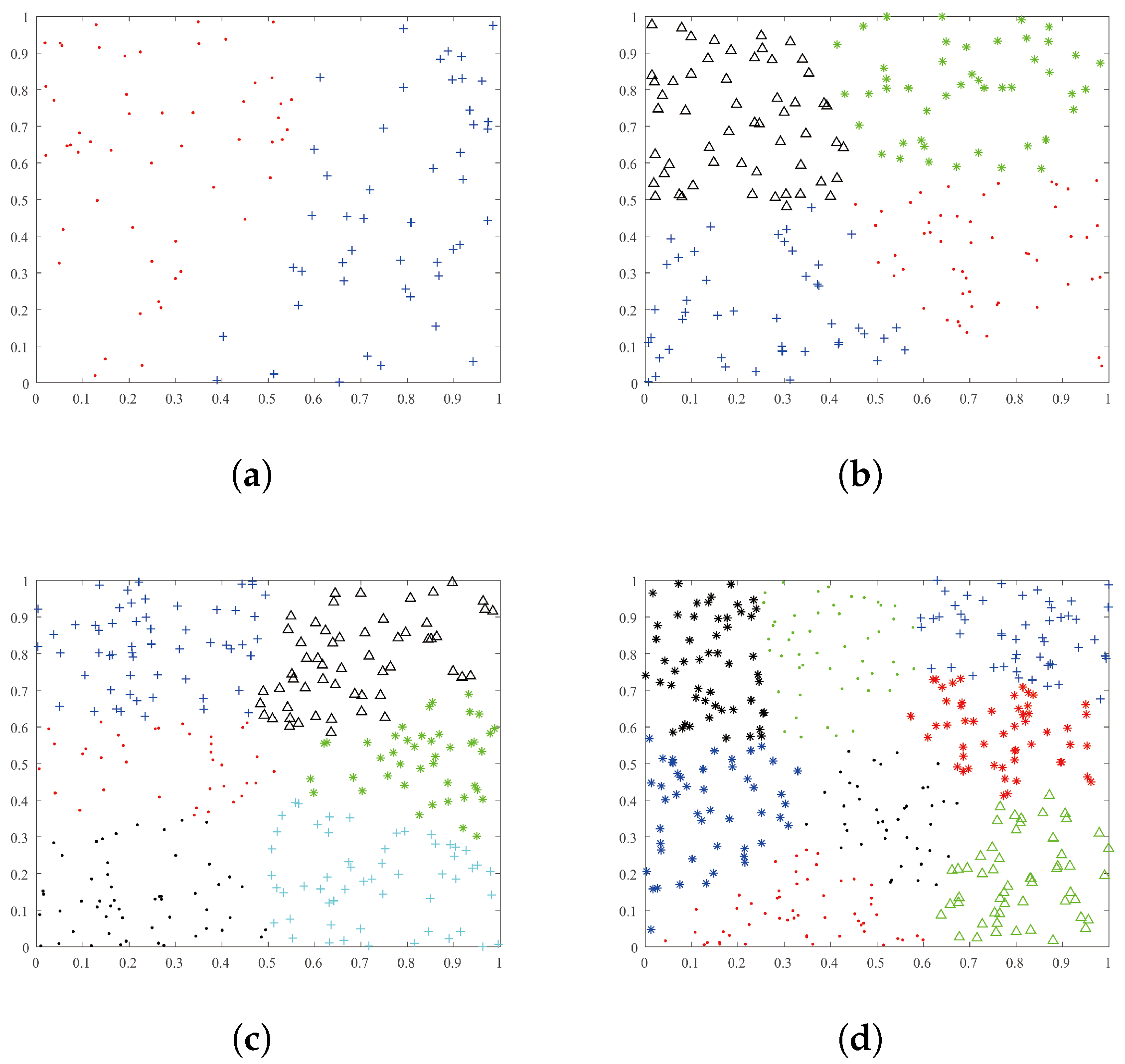
4.2. Numerical Experiment

This section utilizes randomly generated 2D points to conduct the numerical experiment. Figure 1 vividly shows clustering results on various instances numbers with different classes. According to the figure, we conclude as follows:

• The clustering result of our method is satisfactory for different instances with different classes.
• Our method obtains ideal clustering results for multi-class instances.

4.3. Real Datasets Experiment

4.3.1. Evaluation Indices

The clustering performances of are evaluated using four common external performance indices: Normalized Mutual Information (NMI) [31], Accuracy (AC) [31], Adjusted Rand index (ARI) [32] and Purity [33].

The details of these evaluation indices are shown in

Table 3. Definitions of the used cluster validity indices.

Index	Definition	Rule to Indicate the Best Clusters
Normalized Mutual Information (NMI)	$NMI(U,V)=\frac{MI(U,V)}{mean\left(H\right(U),H(V\left)\right)}$ where $MI(U,V)={\sum }_{i=1}^{\left|U\right|}{\sum }_{j=1}^{\left|V\right|}\frac{|U_i\cap V_j|}{N}log\frac{N|U_i\cap V_j|}{|U_i\left|\right|V_j|}$	max
Accuracy (AC)	$AC=\frac{{\sum }_{i=1}^n\delta (s_i,map\left(r_i\right))}{n}$ where $\delta =\left\{\begin{array}{cc}& 1ifx=y\hfill \\ & 0\mathrm{otherwises}.\hfill \end{array}\right.$	max
Adjusted Rand Index (ARI)	$ARI=\frac{RI-E\left(RI\right)}{max\left(RI\right)-E\left(RI\right)}$	max
Purity	$Purity(\Omega ,C)=\frac{1}{N}{\sum }_k{max}_j|w_k\cap c_j|$	max

. In Table 3, H denotes entropy; U and V are the data label and the obtained label of the i-th sample, respectively; $r_i$ and $s_i$ represent pre-label and real-label, respectively; $RI$ denotes the ratio of the correctly clustered data points and all data points. E denotes the expectation; N is the number of instances, $\mathsf{\Omega }$ denotes a forecasting label, C is a real label.

Remarks: The higher the NMI, AC, ARI and Purity, the better the performance.

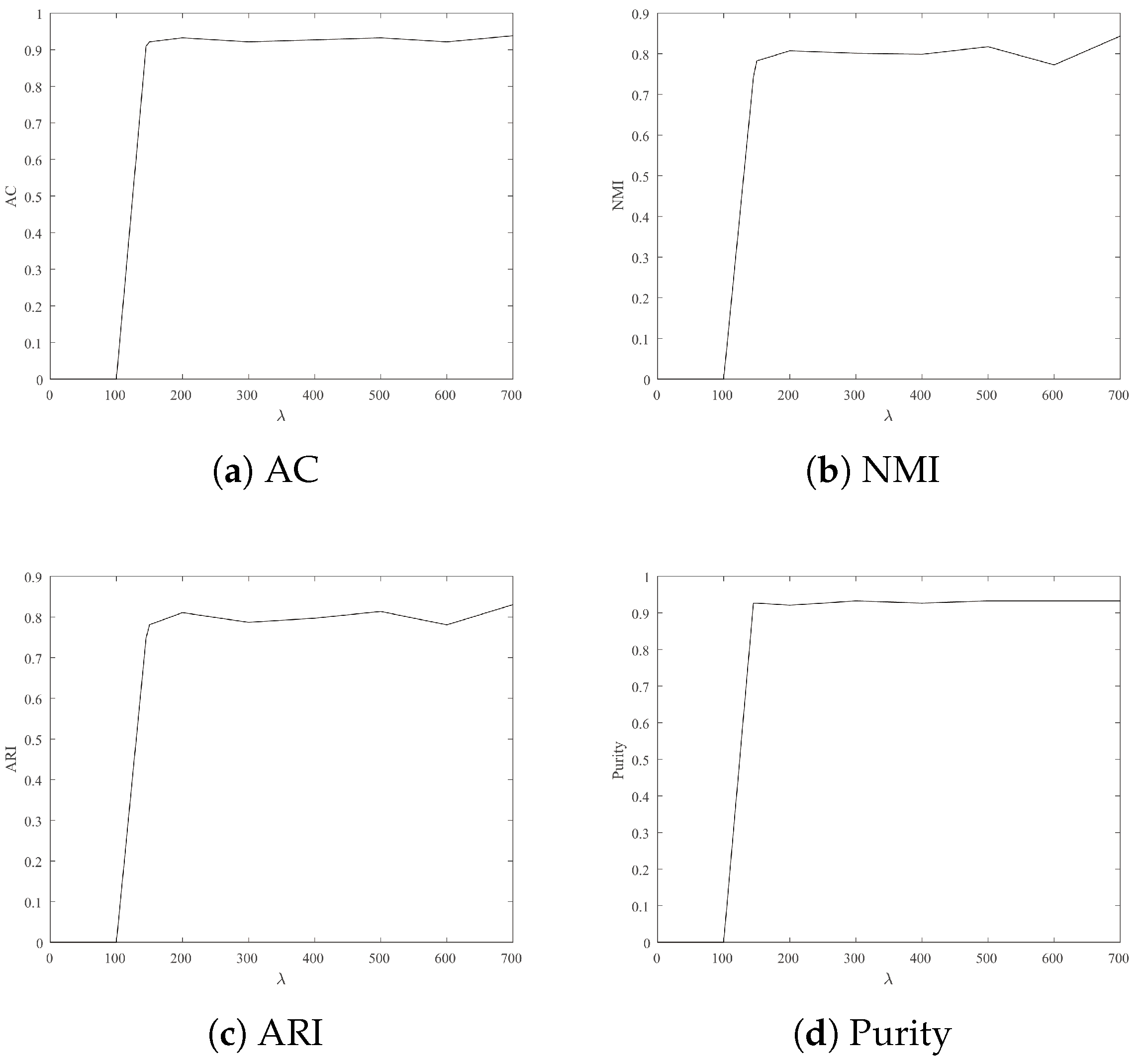
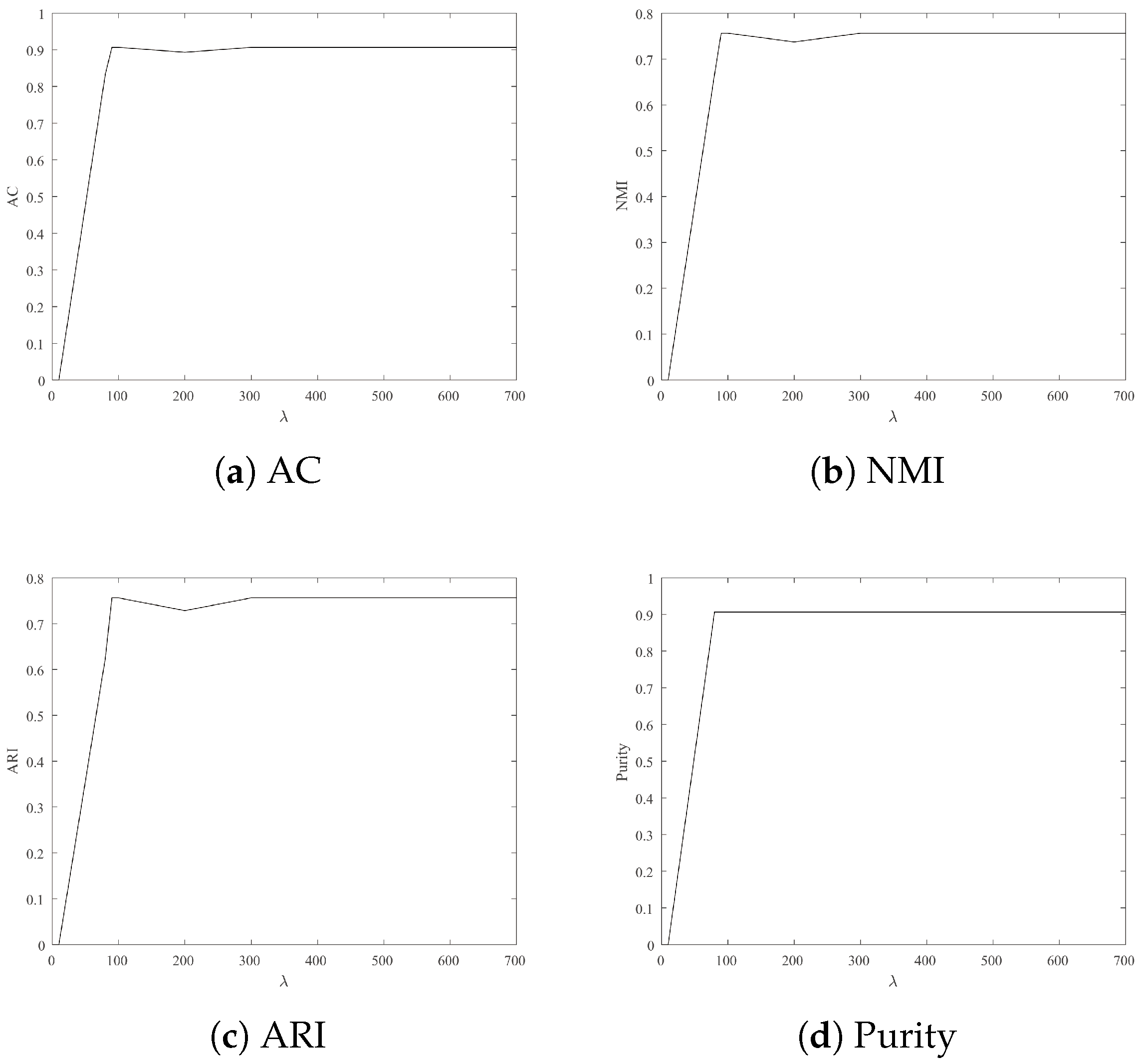
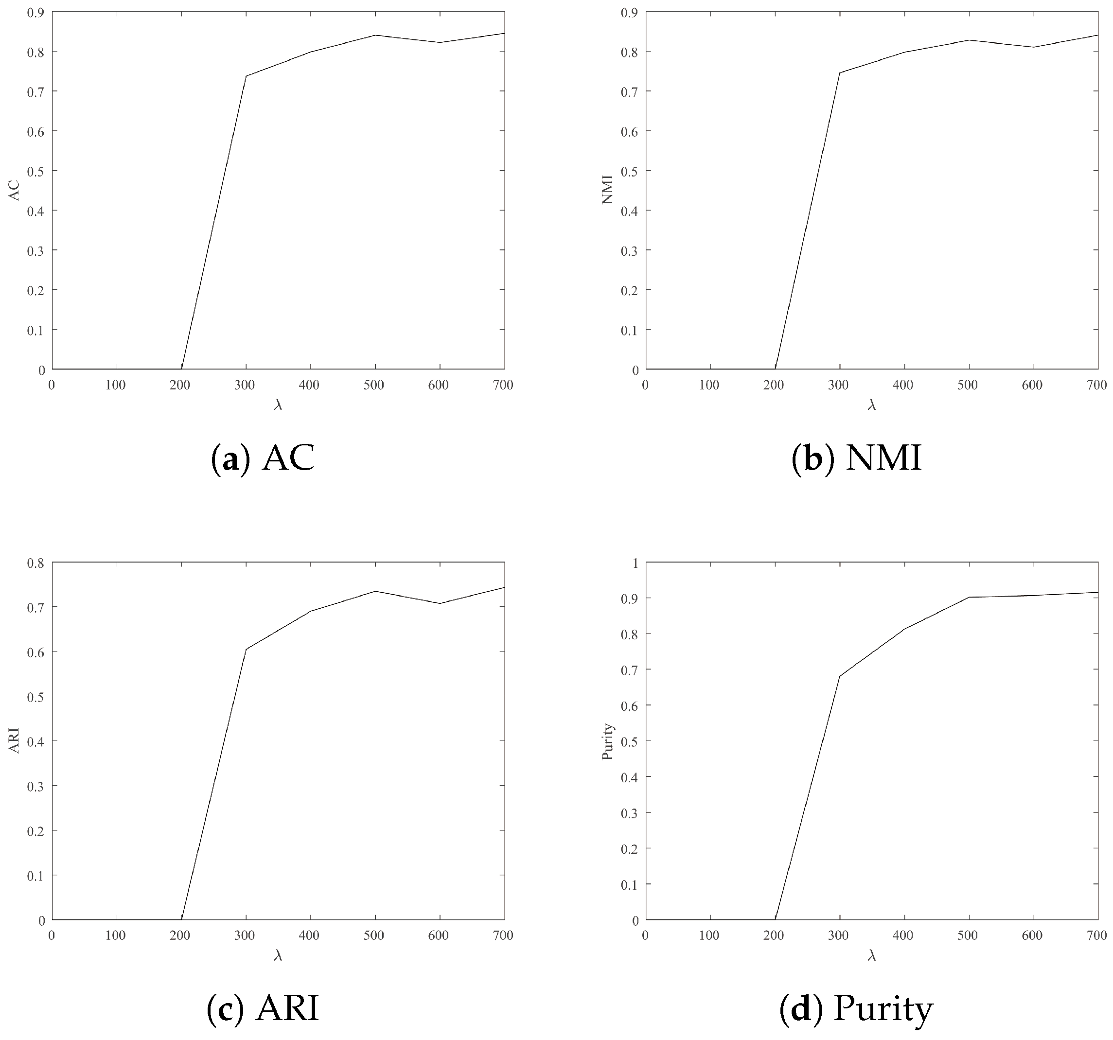
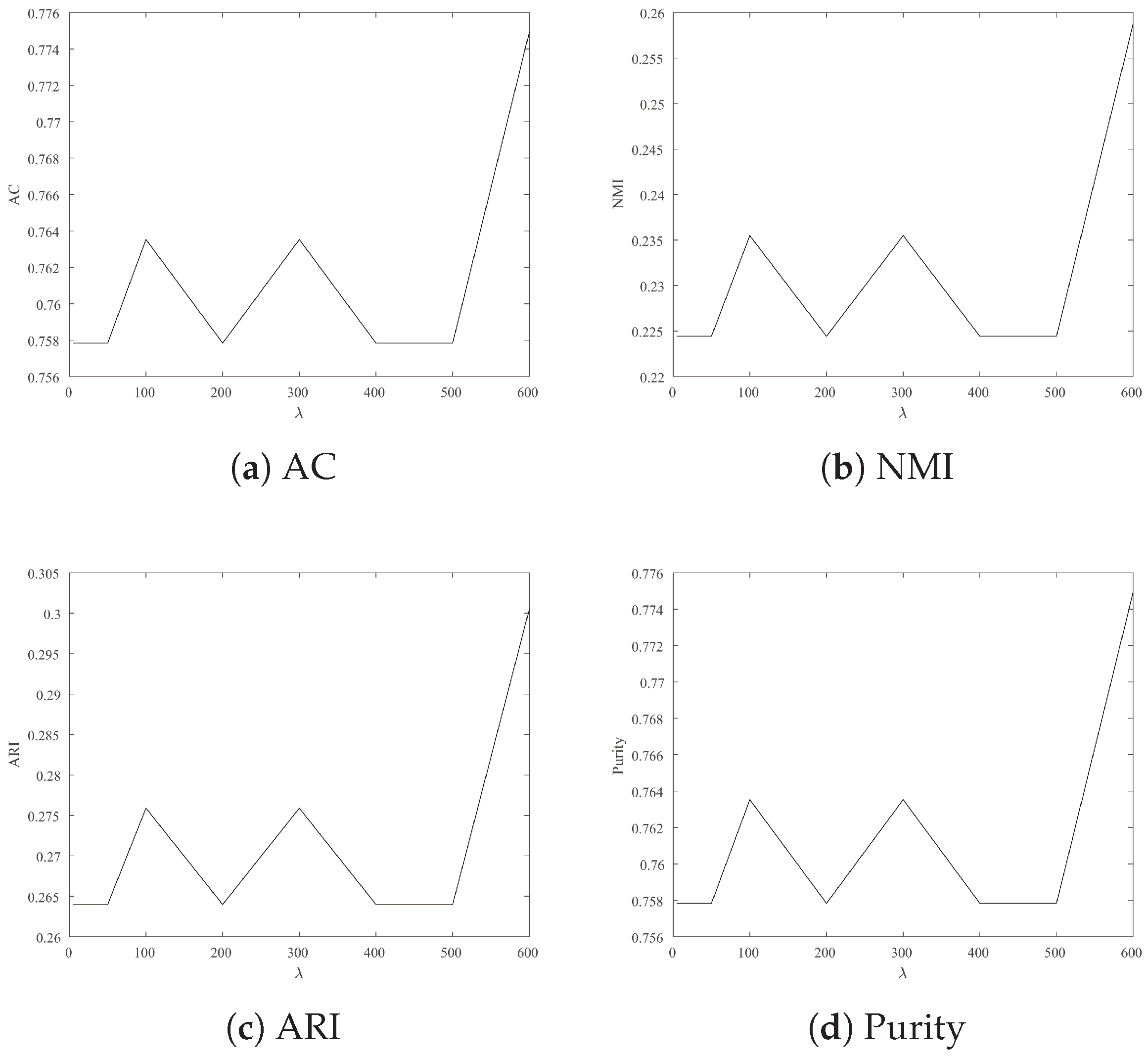
4.3.2. Parameter Sensitivity

To achieve an ideal experiment performance, Figure 2, Figure 3, Figure 4, Figure 5 and Figure 6 show experimental results with different lambda on four datasets. These figures denote two-dimensional images, where x-axis and y-axis denote the various of $\lambda$ and different clustering indexes, respectively. According to Figure 2, Figure 3, Figure 4, Figure 5 and Figure 6, we summarized as follows:

• For Wine, Iris and Seeds, the clustering results are more satisfactory when $\lambda$ is 700.
• For Jacc_face and Ionosphere, the larger $\lambda$ leads to better clustering results.

4.3.3. Experiment Results

Table 4. The experimental results of our proposed method compared to Kmeans, Kmeans$++$ and Isodata in terms of the best, worst, mean and standard deviations performance metric values on Wine (The best result in bold).

Algorithm	CHN	Kmeans	Kmeans$++$	Isodata
NMI(%)	81.40/84.35/77.27 ± 2.10	67.36/77.53/38.50 ± 11.94	67.43/77.53/60.44 ± 7.03	46.93/72.57/30.52 ± 13.48
AC(%)	93.09/93.82/92.13 ± 0.53	84.66/93.26/55.05 ± 11.63	85.62/93.26/81.46 ± 5.30	66.97/92.13/54.49 ± 13.08
ARI(%)	80.96/83.04/78.08 ± 1.47	63.83/79.61/29.99 ± 16.47	62.59/79.61/55.52 ± 11.79	38.86/76.84/17.61 ± 17.84
Purity(%)	93.09/93.82/92.13 ± 0.53	85.84/93.25/66.85 ± 8.46	85.62/93.25/81.46 ± 5.30	69.72/92.13/59.55 ± 11.04

,

Table 5. The experimental results of our proposed method compared to Kmeans, Kmeans$++$ and Isodata in terms of the best, worst, mean and standard deviations performance metric values on Seeds (The best result in bold).

Algorithm	CHN	Kmeans	Kmeans$++$	Isodata
NMI(%)	26.25/22.44/23.26 ± 1.19	20.67/20.38/20.55 ± 0.15	20.67/20.38/20.58 ± 0.14	25.30/2.69/14.35 ± 8.69
AC(%)	77.78/75.78/76.21 ± 0.62	64.10/63.81/63.99 ± 0.15	64.10/63.81/64.10 ± 0.14	68.37/53.00/60.60 ± 3.94
ARI(%)	30.68/26.39/27.30 ± 1.32	6.48/6.12/6.33 ± 0.18	6.48/6.12/6.37 ± 0.17	12.55/−4.79/1.52 ± 5.41
Purity(%)	77.77/75.78/76.21 ± 0.62	64.10/64.10/64.10 ± 0	64.10/64.10/64.10 ± 0	68.37/64.10/64.52 ± 1.35

,

Table 6. The experimental results of our proposed method compared to Kmeans, Kmeans$++$ and Isodata in terms of the best, worst, mean and standard deviations performance metric values on Ionosphere (the best result in bold).

Algorithm	CHN	Kmeans	Kmeans$++$	Isodata
NMI(%)	26.25/22.44/23.26 ± 1.19	20.67/20.38/20.55 ± 0.15	20.67/20.38/20.58 ± 0.14	25.30/2.69/14.35 ± 8.69
AC(%)	77.78/75.78/76.21 ± 0.62	64.10/63.81/63.99 ± 0.15	64.10/63.81/64.10 ± 0.14	68.37/53.00/60.60 ± 3.94
ARI(%)	30.68/26.39/27.30 ± 1.32	6.48/6.12/6.33 ± 0.18	6.48/6.12/6.37 ± 0.17	12.55/−4.79/1.52 ± 5.41
Purity(%)	77.77/75.78/76.21 ± 0.62	64.10/64.10/64.10 ± 0	64.10/64.10/64.10 ± 0	68.37/64.10/64.52 ± 1.35

,

Table 7. The experimental results of our proposed method compared to Kmeans, Kmeans$++$ and Isodata in terms of the best, worst, mean and standard deviations performance metric values on Seeds (the best result in bold).

Algorithm	CHN	Kmeans	Kmeans$++$	Isodata
NMI(%)	67.35/71.02/64.90 ± 2.09	65.37/66.32/64.90 ± 0.68	65.75/66.32/64.90 ± 0.73	48.94/68.49/39.94 ± 8.35
AC(%)	89.57/90.95/88.57 ± 0.82	88.91/89.52/88.57 ± 0.45	89.14/89.53/88.57 ± 0.49	71.52/88.57/54.76 ± 10.71
ARI(%)	71.62/75.06/69.19 ± 2.01	69.99/71.47/69.19 ± 1.08	70.56/71.47/69.19 ± 1.18	46.18/69.64/35.33 ± 10.84
Purity(%)	89.57/90.95/88.57 ± 0.82	88.90/89.52/88.57 ± 0.45	89.14/89.52/88.57 ±0.49	72.90/88.57/62.38 ± 8.90

,

Table 8. The experimental results of our proposed method compared to Kmeans, Kmeans$++$ and Isodata in terms of the best, worst, mean and standard deviations performance metric values on Iris (the best result in bold).

Algorithm	CHN	Kmeans	Kmeans$++$	Isodata
NMI(%)	75.54/75.64/74.65 ± 0.31	74.76/75.14/74.50 ± 0.33	74.82/75.15/74.51 ± 0.33	63.21/78.37/47.81 ± 9.56
AC(%)	90.60/90.67/90 ± 0.21	89.33/89.33/89.33 ± 0	89.33/89.33/89.33 ± 0	76.00/92.00/51.33 ± 11.89
ARI(%)	75.47/75.64/74.20 ± 0.45	72.97/73.02/72.94 ± 0.04	72.98/73.02/72.94 ± 0.04	57.63/78.64/38.43 ± 12.47
Purity(%)	90.67/90.67/90.67 ± 0	89.33/89.33/89.33 ± 0	89.33/92.67/89.33 ± 1.27	77.60/92.67/66.67 ± 8.73

and

Table 9. The experimental results of our proposed method compared to Kmeans, Kmeans$++$ and Isodata in terms of the best, worst, mean and standard deviations performance metric values on Jaffe_face (The best result in bold).

Algorithm	CHN	Kmeans	Kmeans$++$	Isodata
NMI(%)	83.41/89.41/74.41 ± 4.45	82.19/88.88/74.16 ± 4.81	80.43/89.38/70.15 ± 5.57	70.38/83.43/50.79 ± 10.57
AC(%)	83.10/91.50/69.50 ± 6.67	76.85/87.00/65.00 ± 7.06	70.75/91.00/54.50 ± 9.58	64.75/81.00/38.00 ± 14.01
ARI(%)	73.83/83.79/58.28 ± 7.43	68.72/82.42/52.98 ± 9.15	65.08/81.52/48.12 ± 9.01	53.48/73.37/24.32 ± 15.67
Purity(%)	83.75/91.50/72.00 ± 5.76	79.85/87.50/73.00 ± 5.23	75.60/91.00/63.50 ± 7.59	69.30/83.50/46.50 ± 11.73

show the algorithm performance of our method compared to Kmeans, Kmeans$++$ and Isodata in terms of four clustering performance metric values. These tables show the best, worst, mean and standard deviation performance metric values on the four datasets. The clustering result in these tables demonstrate that the our proposed algorithm statistically outperform the other three algorithms in the light of the given cluster evaluation indices. According to these tables, we summarize the results as follows:

• Our method far outperforms other methods in Table 4, Table 6 and Table 9, no matter which evaluation indicator is applied.
• For Table 5 and Table 8, although other methods perform better than our method in some minimum and standard deviation, our method outperforms other methods as a whole.

5. Conclusions and Future Work

In this paper, a neural network clustering algorithm is proposed. The clustering is regarded as a combinatorial optimization problem. The proposed clustering algorithm model applies a CHN to solve and the Hopfield networks are repositioned repeatedly upon their local stability until convergence. The experimental results show that our algorithm is obviously superior to other algorithms on four different datasets. According to Section 4.3, the experiment of parameter sensitivity can conclude that the $\lambda$ is set by experience. Therefore, there is no theory for ensuring $\lambda$. In the future work:

• Other neural networks can be used to solve clustering problems.
• We are exploring how to effectively combine Hopfield Neural Network with Swarm Intelligence methods.

References

1. Shaheen, M.; ur Rehman, S.; Ghaffar, F. Correlation and congruence modulo based clustering technique and its application in energy classification. Sustain. Comput. Inform. Syst. 2021, 30, 100561. [Google Scholar] [CrossRef]
2. Abdullah, D.; Susilo, S.; Ahmar, A.S.; Rusli, R.; Hidayat, R. The application of K-means clustering for province clustering in Indonesia of the risk of the COVID-19 pandemic based on COVID-19 data. Qual. Quant. 2021; Online ahead of print. [Google Scholar] [CrossRef]
3. Yeoh, J.M.; Caraffini, F.; Homapour, E.; Santucci, V.; Milani, A. A clustering system for dynamic data streams based on metaheuristic optimisation. Mathematics 2019, 7, 1229. [Google Scholar] [CrossRef] [Green Version]
4. Ng, A.Y.; Jordan, M.I.; Weiss, Y. On spectral clustering: Analysis and an algorithm. Adv. Neural Inf. Process. Syst. 2002, 14, 849–856. [Google Scholar]
5. Chen, W.Y.; Song, Y.; Bai, H.; Lin, C.J.; Chang, E.Y. Parallel spectral clustering in distributed systems. IEEE Trans. Pattern Anal. Mach. Intell. 2010, 33, 568–586. [Google Scholar] [CrossRef] [PubMed]
6. Chan, P.K.; Schlag, M.D.; Zien, J.Y. Spectral k-way ratio-cut partitioning and clustering. IEEE Trans. Comput.-Aided Des. Integr. Circuits Syst. 1994, 13, 1088–1096. [Google Scholar] [CrossRef]
7. Shi, J.; Malik, J. Normalized cuts and image segmentation. IEEE Trans. Pattern Anal. Mach. Intell. 2000, 22, 888–905. [Google Scholar]
8. Ding, C.H.; He, X.; Zha, H.; Gu, M.; Simon, H.D. A min-max cut algorithm for graph partitioning and data clustering. In Proceedings of the 2001 IEEE International Conference on Data Mining, San Jose, CA, USA, 29 November–2 December 2001; pp. 107–114. [Google Scholar]
9. Nie, F.; Wang, X.; Huang, H. Clustering and projected clustering with adaptive neighbors. In Proceedings of the 20th ACM SIGKDD International Conference on Knowledge Discovery and Data Mining, New York, NY, USA, 24–27 August 2014; pp. 977–986. [Google Scholar]
10. Wang, Y.; Wu, L. Beyond low-rank representations: Orthogonal clustering basis reconstruction with optimized graph structure for multi-view spectral clustering. Neural Netw. 2018, 103, 1–8. [Google Scholar] [CrossRef] [Green Version]
11. Li, X.; Fang, Z. Parallel clustering algorithms. Parallel Comput. 1989, 11, 275–290. [Google Scholar] [CrossRef]
12. Grygorash, O.; Zhou, Y.; Jorgensen, Z. Minimum spanning tree based clustering algorithms. In Proceedings of the 18th IEEE International Conference on Tools with Artificial Intelligence (ICTAI’06), Arlington, VA, USA, 13–15 November 2006; pp. 73–81. [Google Scholar]
13. Dai, X.; Zhang, K.; Li, J.; Xiong, J.; Zhang, N. Robust Graph Regularized Non-negative Matrix Factorization for Image Clustering. ACM Trans. Knowl. Discov. Data 2020, 3, 244–250. [Google Scholar]
14. Dai, X.; Zhang, N.; Zhang, K.; Xiong, J. Weighted Nonnegative Matrix Factorization for Image Inpainting and Clustering. Int. J. Comput. Intell. Syst. 2020, 13, 734–743. [Google Scholar] [CrossRef]
15. Malinen, M.I.; Fränti, P. Balanced K-Means for Clustering. In Joint Iapr International Workshops on Statistical Techniques in Pattern Recognition (SPR) and Structural and Syntactic Pattern Recognition (SSPR); Springer: Berlin/Heidelberg, Germany, 2014; pp. 32–41. [Google Scholar]
16. Bauckhage, C.; Piatkowski, N.; Sifa, R.; Hecker, D.; Wrobel, S. A QUBO Formulation of the k-Medoids Problem. In Proceedings of the LWDA/KDML 2019, Berlin, Germany, 30 September–2 October 2019. [Google Scholar]
17. Date, P.; Arthur, D.; Pusey-NAzzaro, L. QUBO Formulations for Training Machine Learning Models. Sci. Rep. 2020, 11, 10029. [Google Scholar] [CrossRef] [PubMed]
18. Hopfield, J.J.; Tank, D.W. Computing with neural circuits: A model. Science 1986, 233, 625–633. [Google Scholar] [CrossRef] [PubMed] [Green Version]
19. Kamgar-Parsi, B.; Gualtieri, J.; Devaney, J.; Kamgar-Parsi, B. Clustering with neural networks. Biol. Cybern. 1990, 63, 201–208. [Google Scholar] [CrossRef]
20. Mulder, S.A.; Wunsch, D.C. Million city traveling salesman problem solution by divide and conquer clustering with adaptive resonance neural networks. Neural Netw. 2003, 16, 827–832. [Google Scholar] [CrossRef]
21. Bakker, B.; Heskes, T. Clustering ensembles of neural network models. Neural Netw. 2003, 16, 261–269. [Google Scholar] [CrossRef]
22. Du, K.L. Clustering: A neural network approach. Neural Netw. 2010, 23, 89–107. [Google Scholar] [CrossRef] [PubMed]
23. Xu, J.; Xu, B.; Wang, P.; Zheng, S.; Tian, G.; Zhao, J. Self-taught convolutional neural networks for short text clustering. Neural Netw. 2017, 88, 22–31. [Google Scholar] [CrossRef] [PubMed] [Green Version]
24. Talaván, P.M.; Yáñez, J. The generalized quadratic knapsack problem. A neuronal network approach. Neural Netw. 2006, 19, 416–428. [Google Scholar] [CrossRef]
25. Zhang, H.; Wang, Z.; Liu, D. A Comprehensive Review of Stability Analysis of Continuous-Time Recurrent Neural Networks. IEEE Trans. Neural Netw. Learn. Syst. 2014, 25, 1229–1262. [Google Scholar] [CrossRef]
26. Talavan, P.M.; Yanez, J. A continuous Hopfield network equilibrium points algorithm. Comput. Oper. Res. 2005, 32, 2179–2196. [Google Scholar] [CrossRef]
27. Wold, S.; Esbensen, K.; Geladi, P. Principal component analysis. Chemom. Intell. Lab. Syst. 1987, 2, 37–52. [Google Scholar] [CrossRef]
28. Hartigan, J.A.; Wong, M.A. Algorithm AS 136: A k-means clustering algorithm. J. R. Stat. Soc. Ser. C Appl. Stat. 1979, 28, 100–108. [Google Scholar] [CrossRef]
29. Arthur, D.; Vassilvitskii, S. k-means++: The advantages of careful seeding. In Proceedings of the Eighteenth Annual ACM-SIAM Symposium on Discrete Algorithms, New Orleans, LO, USA, 7–9 January 2007. [Google Scholar]
30. Ball, G.H.; Hall, D.J. ISODATA, a Novel Method of Data Analysis and Pattern Classification; Stanford Research Institute: Menlo Park, CA, USA, 1965. [Google Scholar]
31. Cai, D.; He, X.; Han, J. Document clustering using locality preserving indexing. IEEE Trans. Knowl. Data Eng. 2005, 17, 1624–1637. [Google Scholar] [CrossRef] [Green Version]
32. Santos, J.M.; Embrechts, M. On the use of the adjusted rand index as a metric for evaluating supervised classification. In International Conference on Artificial Neural Networks; Springer: Berlin/Heidelberg, Germany, 2009; pp. 175–184. [Google Scholar]
33. Rendon, E.; Abundez, I.; Arizmendi, A.; Quiroz, E.M. Internal versus external cluster validation indexes. Int. J. Comput. Commun. 2011, 5, 27–34. [Google Scholar]
Figure 1. Numerical experiments are conducted on 100, 200, 300 and 400 instances with 2, 4, 6 and 8 classes, respectively. (a) Numerical experiments are conducted on 100 instances with 2 classes; (b) Numerical experiments are conducted on 200 instances with 4 classes; (c) Numerical experiments are conducted on 300 instances with 6 classes. (d) Numerical experiments are conducted on 400 instances with 8 classes.
Mathematics 10 00944 g001
Figure 2. Clustering result: AC, NMI, ARI and Purity from Wine with different λ .
Mathematics 10 00944 g002
Figure 3. Clustering result: AC, NMI, ARI and Purity from Iris with different λ .
Mathematics 10 00944 g003
Figure 4. Clustering result: AC, NMI, ARI and Purity from Seeds with different λ .
Mathematics 10 00944 g004
Figure 5. Clustering result: AC, NMI, ARI and Purity from Jacc_face with different λ .
Mathematics 10 00944 g005
Figure 6. Clustering result: AC, NMI, ARI and Purity from Ionosphere with different λ .
Mathematics 10 00944 g006