Parameter Identification and the Finite-Time Combination–Combination Synchronization of Fractional-Order Chaotic Systems with Different Structures under Multiple Stochastic Disturbances

Abstract

This paper researches the issue of the finite-time combination-combination (C-C) synchronization (FTCCS) of fractional order (FO) chaotic systems under multiple stochastic disturbances (SD) utilizing the nonsingular terminal sliding mode control (NTSMC) technique. The systems we considered have different characteristics of the structures and the parameters are unknown. The stochastic disturbances are considered parameter uncertainties, nonlinear uncertainties and external disturbances. The bounds of the uncertainties and disturbances are unknown. Firstly, we are going to put forward a new FO sliding surface in terms of fractional calculus. Secondly, some suitable adaptive control laws (ACL) are found to assess the unknown parameters and examine the upper bound of stochastic disturbances. Finally, combining the finite-time Lyapunov stability theory and the sliding mode control (SMC) technique, we propose a fractional-order adaptive combination controller that can achieve the finite-time synchronization of drive-response (D-R) systems. In this paper, some of the synchronization methods, such as chaos control, complete synchronization, projection synchronization, anti-synchronization, and so forth, have become special cases of combination-combination synchronization. Examples are presented to verify the usefulness and validity of the proposed scheme via MATLAB.

1. Introduction

Chaos is not an accidental or individual event, but a universal existence in various macro and micro systems in the universe. It promotes and relies on other sciences, which derive many interdisciplinary subjects, such as chaotic meteorology, chaotic economics, chaotic mathematics, and so forth. Because chaos is ubiquitous in many systems, the research on chaotic systems has drawn widespread attention of scholars. Thanks to the nonlinear nature of the chaotic system and the sensitivity to the initial value, the control and synchronization to the chaotic system has become a very difficult problem. Up to now, many valid synchronization methods were researched, such as drive-response synchronization [1], projective synchronization [2,3], adaptive fuzzy control [4,5,6], neural network synchronization [7,8], feedback synchronization [9] and pulse synchronization [10,11], sliding mode control [12,13] and so forth.

Some scholars have taken the above methods into consideration for the synchronization problem of FO chaotic systems [14,15,16,17,18,19]. However, the above research content does not consider the uncertainties of the system and external disturbances. Since the chaotic system is sensitive to the initial values; in practical applications, it is inevitable that the orbit of the system will change dramatically due to some small disturbances. One has adopted the active nonlinear control method to address the issue of modified projective synchronization for the FO chaotic systems with noise disturbance in Ref. [20]. Qin et al. established the system with the unknown nonlinear functions and uncertainties which are addressed by fuzzy logic method [4]. Meanwhile, replacing the FO chaotic systems in Ref. [4] with non-identical complex FO chaotic systems, the adaptive sliding mode synchronization has developed in Ref. [21]. Luo et al. derived some novel sufficient conditions for chaos synchronization of FO chaotic systems with nonlinear uncertainties and external disturbances [22]. In Ref. [23], the authors researched the multi-state uncertain synchronization of chaotic systems in which the structure is non-identical, parameters are unknown, and systems have a time-varying delay. This means the synchronization of the single master system with multiple slave systems which have more potential applications in real life. However, the master–slave system they considered was an integer order system and the synchronization of both systems is asymptotic and takes place in infinite time. This is also the case in Ref. [24]. It is generally found that fractional derivatives are better suited to describe memory and hereditary characteristics of different materials and processes than integer derivatives [25]. Mirrezapour et al. [26] used the sliding mode control to synchronize fractional-order chaotic systems with uncertainties and affected by disturbance. In Ref. [26], a new fractional sliding mode controller according to nonlinear FO controllers is proposed. However, there are some disadvantages here. Firstly, the author did not consider the effect of unknown parameters on the system. Then, from the numerical simulation results (synchronization errors converges to zero at $t=10$ (approx)), it can be seen that the controller is not very effective in overcoming uncertainty and disturbance. On the contrary, the nonsingular terminal sliding mode control in our paper has a better transient performance, easy realization, rapid response, and insensitivity to external disturbances and so on. Of course, there are some studies on uncertain parameters of systems [27,28,29]. However, it can be seen from the above that for the uncertainties of the system, that is, parameter uncertainties and nonlinear uncertainties, and the influence of external disturbances on the system, most authors study some of the situations while a few authors have considered the three of them at the same time [30,31,32]. Furthermore, the above mentioned papers reveal that the convergence of the ideal dynamics is promised without time limit. We know that the finite time convergence with even existing disturbances has merits in strengthening the robustness, getting over the disturbance [33] and improving the security of information transmission in the field of chaotic communication [34]. Some more theoretical results about the synchronization of FO chaotic systems with uncertainties and external disturbances in finite-time can be seen in [35,36,37,38,39,40,41,42]. At present, with full consideration of system uncertainties and external disturbances in the given time as well as the unknown system parameters, no researchers have considered this situation.

There is another fact that we must note that the aforementioned papers focused on the single D-R system for the synchronization scheme. There are relatively few studies on multi-drive systems and multi-response systems, as well as the combination synchronization of each system. Actually, in engineering, communication theory, physics, electrical and many other fields, the combination–combination synchronization has more potential applications [43,44]. Just take the secure communication, for example, the transmitting signals can be understood as two basic ways. The first is to divide the transmission signals into multiple parts, each loaded with different drive systems. For example, assume the transmitted signal is $cost$, the signal $cost$ can be broken down into two parts: $\frac{1}{3}cost$ and $\frac{2}{3}cost$. The signal $\frac{1}{3}cost$ can be delivered to the first drive system, while $\frac{2}{3}cost$ can be delivered to the second drive system. The second way is to break down time into different intervals. Let the signals in different intervals load in different drive systems. It is clear to observe that the traditional master–slave synchronization schemes (one to one system) do not satisfy the above communication signals but can be transferred in our model. Thus, it is imperative to pay more attention to the synchronization research of multi-systems. Sun et al. [42] realized the parameter identification and C-C synchronization in a finite time. In [24], the authors handle a hybrid projective C-C synchronization scheme between four specific hyper-chaotic systems utilizing SMC. The idea of dual C-C multi switching synchronization adopted the eight chaotic systems was addressed in [45]. The global exponential multi switching combination synchronization was introduced in terms of three different chaotic systems, in [46]. There are also some papers here that also mention the issue of C-C synchronization [47,48,49,50]. However, the systems they consider are all integer order chaotic systems and some of them do not consider the SD.

In response to this situation, we are going to consider the finite-time combination–combination (C-C) synchronization (FTCCS) of FO chaotic systems with different structures and unknown parameters under multiple SD via the NTSMC technique. The multiple SD are explained as parameter uncertainties, nonlinear uncertainties and external disturbances. In the light of finite-time Lyapunov stability theory and the SMC technique, we propose an FO adaptive combination controller and some appropriate ACL.

Compared with other references, there are four advantages of the proposed method: (1) The finite-time control theory is different from the traditional stability theory and its control structure can be regarded as closed-loop feedback control. The complexity of the finite-time controller is relatively high, which is reflected in the anti-interference ability to the outside world and the robustness to the uncertainty of the system itself; (2) This paper extends the traditional drive-response synchronization schemes (single drive-response system) to combination–combination synchronization schemes. Thus, when the specific parameter values are gained to the D-R systems, the corresponding system or systems’ combination are chose. The controller does not need to be redesigned for two systems or systems’ combinations for every application. This not only has a wider range of applications but also saves too much time and effort. This advantage is reflected in Corollaries 1–3 in the paper; (3) In communication theory, comparing the traditional transmission model with the combination-combination synchronization model, our method has stronger anti-attack ability and anti-translated capability; (4) The nonsingular terminal sliding mode control avoids the singularity problem effectively that terminal sliding mode control (TSMC) would have and retains the characteristic of the finite-time convergence. Besides, the NTSMC has higher control accuracy than linear sliding mode control (SMC); (5) Based on the nonsingular terminal sliding mode control (NTSMC) and adaptive control, the combination–combination drive-response systems with unknown parameters and multiple stochastic disturbances is considered. The controller and parameter updating laws are designed to make the state of drive-response system gradually stable within a finite time. Our controller has good robustness and anti-interference performance.

This article is organized as follows. In Section 2, some definitions, lemmas and stability theories that need to be used are introduced. In Section 3, problem statements and assumptions are given. In Section 4, sliding mode synchronization controller and adaptive control laws are designed. In Section 5, the numerical simulations proved that our method is effective. In Section 6, there is a conclusion.

2. Preliminaries

2.1. Definitions and Lemmas of Fractional Derivative

Next, let us present the Riemann–Liouville (R-L) derivative and the Caputo derivative, which are equivalent if and only if the order $\alpha$ is a negative real number and a positive integer. The R–L definition is best suited for theoretical analysis and can simplify the computation of FO derivatives. The Caputo is more relevant to modern engineering and makes Laplace’s transformation more concise. Thus, we only display the mathematical expression of the Caputo derivative with order $\alpha$.

Definition 1

([51]). The mathematical expression of the fractional integral of the function $f\left(t\right)$ is following:

$$\begin{array}{c}\hfill I_t^{\alpha }f\left(t\right)={\displaystyle \frac{1}{\Gamma \left(\alpha \right)}}{\int }_a^t{\displaystyle \frac{f\left(\upsilon \right)}{{(t-\upsilon )}^{1-\alpha }}}d\upsilon ,\end{array}$$

(1)

where $\Gamma \left(\alpha \right)$ indicates the Gamma function.

Definition 2

([51]). The mathematical expression of Caputo derivative with order α is given as:

$$\begin{array}{c}\hfill {}_a^C{D}_t^{\alpha }f\left(t\right)=\frac{1}{\Gamma (p-\alpha )}{\int }_a^t{(t-\upsilon )}^{p-\alpha -1}{f}^{\left(p\right)}\left(\upsilon \right)d\upsilon ,\end{array}$$

(2)

where $p-1<\alpha <p,p\in {\mathbb{Z}}^{+}$.

Lemma 1

([18]). When $\mathit{x}\left(t\right)\in {\mathbb{R}}^n$ has a continuous first derivative, then

$$\begin{array}{c}\hfill {}_a{D}_t^{\alpha }\left({\displaystyle \frac{1}{2}}{\mathit{x}}^T\left(t\right)Q\mathit{x}\left(t\right)\right)\le {\mathit{x}}^{T}Q{}_a{D}_t^{\alpha }\mathit{x}\left(t\right),\end{array}$$

(3)

where $\alpha \in (0,1)$ and $Q\in R^n\times R^n$ indicate a positive definite matrix.

Lemma 2

([52]). For any real constants $a_i,i=1,2,\cdots ,n$ and $\sigma \in (0,1)$, the following inequality exists:

$$\begin{array}{c}\hfill (|a_1|+|a_2|+\cdots +|a_n{|)}^{\sigma }\le |a_1{|}^{\sigma }+|a_2{|}^{\sigma }+\cdots +{|a_n|}^{\sigma }.\end{array}$$

(4)

2.2. Stability Theories of Fractional Order System

It follows that, if most things around us are nonlinear, we write the FO nonlinear system to be:

$$\begin{array}{cc}\hfill {}_0{D}_t^{\alpha }\mathit{x}\left(t\right)& =\mathit{f}(t,\mathit{x}(t\left)\right),\hfill \end{array}$$

(5)

where $\alpha \in (0,1)$, $\mathit{f}={(f_1,f_2,\cdots ,f_n)}^T$, $\mathit{x}\left(t\right)\in {\mathbb{R}}^n$ and $f:[t_0,\infty ]\times \Omega \to {\mathbb{R}}^n$ satisfies the requirements of Lipschitz conditions; the initial value is $x\left(t_0\right)=x_0,t_0\ge 0$. The equilibrium point ${\mathit{x}}^{*}$ of (5) can be calculated from $\mathit{f}\left({\mathit{x}}^{*}\right)=0$.

Theorem 1

([53]). Suppose that $\mathbb{D}\in {\mathbb{R}}^n$ is a domain that contains the origin. If there exists a locally bounded Lyapunov function $V(t,\mathit{x}):[t_0,\infty ]\times \mathbb{D}\to \mathbb{R}$ which meets the local Lipschitz condition about x adapting to

$$\begin{array}{c}\hfill {\eta }_1{(\parallel \mathit{x}\parallel }^a)\le V(t,\mathit{x})\le {\eta }_2{(\parallel \mathit{x}\parallel }^{ab}),\end{array}$$

(6)

$$\begin{array}{c}\hfill {}_0{D}_t^{\alpha }V(t,\mathit{x})\le -{\eta }_3{(\parallel \mathit{x}\parallel }^{ab}),\end{array}$$

(7)

where $\alpha \in (0,1)$, $a>0$, $b>0$, ${\eta }_i(i=1,2,3)>0$, then the system (5) is called Mittag-Leffler stable.

Theorem 2.

Suppose that $\mathbb{D}\subset {\mathbb{R}}^n$ is a domain that contains the origin. If there is a locally bounded Lyapunov function $V(t,\mathit{x}):[t_0,\infty ]\times \mathbb{D}\to \mathbb{R}$ that meets the local Lipschitz condition about x adapting to

$$\begin{array}{c}\hfill \left(1\right){\eta }_1{(\parallel \mathit{x}\parallel }^a)\le V(t,\mathit{x})\le {\eta }_2{(\parallel \mathit{x}\parallel }^{ab}),\\ \hfill {\left(2\right)}_0{D}_t^{\alpha }V(t,\mathit{x})\le -{\eta }_3{(\parallel \mathit{x}\parallel }^{ab}),\\ \hfill {\left(3\right)}_0{D}_t^{\alpha }V(t,\mathit{x})\le -k{V}^{1/\beta }(t,\mathit{x}),\end{array}$$

(8)

where $\alpha \in (0,1)$, $a>0$, $b>0$, $k>0$, $\beta >1$, $\alpha >1/\beta$, ${\eta }_i(i=1,2,3)>0$, then the system (5) is called finite-time stable. The system (5) will be stabilized in time T given by:

$$\begin{array}{c}\hfill T\le {\left[V^{\alpha -\frac{1}{\beta }}(0,\mathit{x})\frac{\Gamma (1-\frac{1}{\beta })\Gamma (1+\alpha )}{\Gamma (\alpha -\frac{1}{\beta }+1)k}\right]}^{\frac{1}{\alpha }}.\end{array}$$

(9)

Proof. 

It is clear that the conditions (1) and (2) in Theorem 2 satisfy Theorem 1. Thus, the system (5) is Mittag–Leffler stable. Then, there is an equilibrium point $x\left(t_0\right)$ for system (5). According to condition (3), one obtained

$$\begin{array}{c}\hfill V^{-1/\beta }(t,\mathit{x}){[}_{t_0}{D}_t^{\alpha }V(t,\mathit{x})]\le -k.\end{array}$$

(10)

For convenience, let $\nu =1/\beta$. Based on the property of Caputo fractional derivatives $D_t^{\alpha }{x}^{\mu }=\frac{\Gamma (\mu +1)}{\Gamma (\mu +1-\alpha )}{x}^{\mu -\alpha }{D}_t^{\alpha }x$ [54], we get

$$\begin{array}{c}\hfill {}_a{D}_t^{\alpha }{V}^{\alpha -\nu }(t,\mathit{x})=\frac{\Gamma (\alpha -\nu +1)}{\Gamma (1-\nu )}{V}^{-\nu }(t,\mathit{x}){}_a{D}_t^{\alpha }V(t,\mathit{x})\end{array}$$

(11)

$$\begin{array}{c}\hfill V^{-\nu }(t,\mathit{x}){}_a{D}_t^{\alpha }V(t,\mathit{x})=\frac{\Gamma (1-\nu )}{\Gamma (\alpha -\nu +1)}{}_a{D}_t^{\alpha }{V}^{\alpha -\nu }(t,\mathit{x}).\end{array}$$

(12)

Then,

$$\begin{array}{c}\hfill \frac{\Gamma (1-\nu )}{\Gamma (\alpha -\nu +1)}{}_a{D}_t^{\alpha }{V}^{\alpha -\nu }(t,\mathit{x})\le -k,\end{array}$$

(13)

$$\begin{array}{c}\hfill {}_a{D}_t^{\alpha }{V}^{\alpha -\nu }(t,\mathit{x})\le -k\frac{\Gamma (\alpha -\nu +1)}{\Gamma (1-\nu )}.\end{array}$$

(14)

Integrating (14) from 0 to T gives:

$$\begin{array}{c}\hfill V^{\alpha -\nu }(T,\mathit{x})-V^{\alpha -\nu }(0,\mathit{x})\le -k\frac{\Gamma (\alpha -\nu +1)}{\Gamma (1-\nu )\Gamma (1+\alpha )}{T}^{\alpha }.\end{array}$$

(15)

Time T can be expressed as:

$$\begin{array}{c}\hfill T\le {\left[V^{\alpha -\nu }(0,\mathit{x})\frac{\Gamma (1-\nu )\Gamma (1+\alpha )}{\Gamma (\alpha -\nu +1)k}\right]}^{\frac{1}{\alpha }}.\end{array}$$

(16)

Namely,

$$\begin{array}{c}\hfill T\le {\left[V^{\alpha -\frac{1}{\beta }}(0,\mathit{x})\frac{\Gamma (1-\frac{1}{\beta })\Gamma (1+\alpha )}{\Gamma (\alpha -\frac{1}{\beta }+1)k}\right]}^{\frac{1}{\alpha }}.\end{array}$$

(17)

□

3. Problem Description and Assumptions

In this chapter, since the the initial values have a great influence on the initial values, in practical application, it is inevitable that the orbit of the system will change dramatically due to some small disturbances. Therefore, it is reasonable to treat them as bounded. This will also make our theory easier to understand.

The FO D-R systems with uncertainties and external disturbance are demonstrated as:

The two drive systems

$$\begin{array}{cc}\hfill {}_0{D}_t^{\mathit{\alpha }}{\mathit{x}}_1\left(t\right)& ={\mathit{F}}_1\left({\mathit{x}}_1\left(t\right)\right)({\mathit{\theta }}_1+\Delta {\mathit{\theta }}_1)+{\mathit{f}}_1\left({\mathit{x}}_1\left(t\right)\right)+\Delta {\mathit{f}}_1\left({\mathit{x}}_1\left(t\right)\right)+{\mathit{d}}_1({\mathit{x}}_1,t),\hfill \end{array}$$

(18)

$$\begin{array}{cc}\hfill {}_0{D}_t^{\mathit{\alpha }}{\mathit{x}}_2\left(t\right)& ={\mathit{F}}_2\left({\mathit{x}}_2\left(t\right)\right)({\mathit{\theta }}_2+\Delta {\mathit{\theta }}_2)+{\mathit{f}}_2\left({\mathit{x}}_2\left(t\right)\right)+\Delta {\mathit{f}}_2\left({\mathit{x}}_2\left(t\right)\right)+{\mathit{d}}_2({\mathit{x}}_2,t).\hfill \end{array}$$

(19)

and the two response systems

$$\begin{array}{cc}\hfill {}_0{D}_t^{\mathit{\alpha }}{\mathit{y}}_1\left(t\right)& ={\mathit{G}}_1\left({\mathit{y}}_1\left(t\right)\right)({\mathit{\vartheta }}_1+\Delta {\mathit{\vartheta }}_1)+{\mathit{g}}_1\left({\mathit{y}}_1\left(t\right)\right)+\Delta {\mathit{g}}_1\left({\mathit{y}}_1\left(t\right)\right)+{\mathit{\mu }}_1({\mathit{y}}_1,t)+{\mathit{u}}_1\left(t\right),\hfill \end{array}$$

(20)

$$\begin{array}{cc}\hfill {}_0{D}_t^{\mathit{\alpha }}{\mathit{y}}_2\left(t\right)& ={\mathit{G}}_2\left({\mathit{y}}_2\left(t\right)\right)({\mathit{\vartheta }}_2+\Delta {\mathit{\vartheta }}_2)+{\mathit{g}}_2\left({\mathit{y}}_2\left(t\right)\right)+\Delta {\mathit{g}}_2\left({\mathit{y}}_2\left(t\right)\right)+{\mu }_{\mathit{2}}({\mathit{y}}_2,t)+{\mathit{u}}_2\left(t\right),\hfill \end{array}$$

(21)

where ${\mathit{\theta }}_i={({\theta }_{1i},{\theta }_{2i},\cdots ,{\theta }_{ni})}^T$ and ${\mathit{\vartheta }}_i={({\vartheta }_{1i},{\vartheta }_{2i},\cdots ,{\vartheta }_{ni})}^T$ are the vectors of system parameters; ${\mathit{x}}_i\left(t\right)={(x_{1i},x_{2i},\cdots ,x_{ni})}^T$ and ${\mathit{y}}_i\left(t\right)={(y_{1i},y_{2i},\cdots ,y_{ni})}^T$; ${\mathit{F}}_i\left({\mathit{x}}_i\left(t\right)\right)={({\mathit{F}}_{1i},{\mathit{F}}_{2i},\cdots ,{\mathit{F}}_{ni})}^T,{\mathit{G}}_i\left({\mathit{y}}_i\left(t\right)\right)={({\mathit{G}}_{1i},{\mathit{G}}_{2i},\cdots ,{\mathit{G}}_{ni})}^T,$ ${\mathit{F}}_{ji},{\mathit{G}}_{ji}\in {\mathbb{R}}^{1\times n},j=1,2,\cdots ,n$, ${\mathit{f}}_i\left({\mathit{x}}_i\left(t\right)\right)={(f_{1i},f_{2i},\cdots ,f_{ni})}^T,{\mathit{g}}_i\left({\mathit{y}}_i\left(t\right)\right)={(g_{1i},g_{2i},\cdots ,g_{ni})}^T$ are the nonlinear continuous functions; ${\mathit{d}}_i\left({\mathit{x}}_i\right)={(d_{1i},d_{2i},\cdots ,d_{ni})}^T$ and ${\mathit{\mu }}_i\left({\mathit{y}}_i\right)={(u_{1i},u_{2i},\cdots ,u_{ni})}^T$ are the external disturbances; ${\alpha }_i\in (0,1)$ represents the fractional order; $\Delta {\mathit{\theta }}_i$ and $\Delta {\mathit{\vartheta }}_i$, $\Delta {\mathit{f}}_i\left({\mathit{x}}_i\left(t\right)\right)$ and $\Delta {\mathit{g}}_i\left({\mathit{y}}_i\left(t\right)\right)$, are the parameter uncertainties and the nonlinear uncertainties. ${\mathit{u}}_i\left(t\right)={(u_{1i},u_{2i},\cdots ,u_{ni})}^T$ are the controllers. Then all of above satisfy $i=1,2$.

Definition 3.

Suppose that $A,B,C,D\in {\mathbb{R}}^n\times {\mathbb{R}}^n,C\ne 0$, or $D\ne 0$ are four constant matrices, then for $T>0$, we have

$$\begin{array}{cc}\hfill \underset{t\to T}{lim}\parallel \mathit{e}\left(t\right)\parallel & =\underset{t\to T}{lim}\parallel C{\mathit{y}}_1\left(t\right)+D{\mathit{y}}_2\left(t\right)-A{\mathit{x}}_1\left(t\right)-B{\mathit{x}}_2\left(t\right)\parallel =0,t<T,\hfill \\ \hfill \parallel \mathit{e}\left(t\right)\parallel & =0,t\ge T.\hfill \end{array}$$

(22)

Then the FO error system, between a combination of drive systems (18), (19) and combination of response systems (20), (21), can reach FTCCS.

Remark 1.

The matrices $A,B,C,D\in {\mathbb{R}}^n\times {\mathbb{R}}^n$$C\ne 0$, or $D\ne 0$ indicating in (22) are named as the scaling matrices. They can also have different meanings, either as constant matrices or as functions of state variables ${\mathit{x}}_1$, ${\mathit{x}}_2$, ${\mathit{y}}_1$ and ${\mathit{y}}_2$.

Remark 2.

If $C=D=I$, $A=B=\lambda I$, then it will be transformed into finite-time C-C complete synchronization with multiple SD for $\lambda =1$; It will be transformed into finite-time C-C anti-synchronization with multiple SD for $\lambda =-1$; What’s more, if $A=C=0,D=I,B=\lambda I$, then it will be transformed into finite-time combination complete synchronization with multiple SD for $\lambda =1$, the finite-time combination anti-synchronization with multiple SD for $\lambda =-1$.

Remark 3.

If $C=0,A=0$ or $C=0,B=0$ or $D=0,A=0$ or $D=0,B=0$, then the issue of finite-time C-C synchronization with multiple SD will be transformed into the issue of finite-time synchronization with multiple SD.

Remark 4.

If $A=0,D=0,C=I$ or $A=0,C=0,D=I$ or $B=0,D=0,C=I$ or $B=0,C=0,D=I$, then it will be transformed into finite-time combination projective synchronization.

Remark 5.

It is supposed that $A=0,B=0,C=0$ or $A=0,B=0,D=0$, then finite-time C-C synchronization with multiple SD will be transformed into the issue of chaos control with multiple SD in the finite time.

Remark 6.

Based on all the above synchronization methods, we can also consider $\Delta {\mathit{\theta }}_i=0,\Delta {\mathit{\vartheta }}_i=0$, or $\Delta {\mathit{f}}_i\left({\mathit{x}}_i\left(t\right)\right)=0,\Delta {\mathit{g}}_i\left({\mathit{y}}_i\left(t\right)\right)=0$, or ${\mathit{d}}_i({\mathit{x}}_i,t)=0,{\mathit{\mu }}_i({\mathit{y}}_i,t)=0$ or $\Delta {\mathit{\theta }}_i=0,\Delta {\mathit{\vartheta }}_i=0,\Delta {\mathit{f}}_i\left({\mathit{x}}_i\left(t\right)\right)=0,\Delta {\mathit{g}}_i\left({\mathit{y}}_i\left(t\right)\right)=0$ or $\Delta {\mathit{\theta }}_i=0,\Delta {\mathit{\vartheta }}_i=0,{\mathit{d}}_i({\mathit{x}}_i,t)=0,{\mathit{\mu }}_i({\mathit{y}}_i,t)=0$, or ${\mathit{d}}_i({\mathit{x}}_i,t)=0,{\mathit{\mu }}_i({\mathit{y}}_i,t)=0,\Delta {\mathit{f}}_i\left({\mathit{x}}_i\left(t\right)\right)=0,\Delta {\mathit{g}}_i\left({\mathit{y}}_i\left(t\right)\right)=0$, or all of the uncertainties and external disturbance equal to zero for $i=1,2$.

Remark 7.

Starting from Definition 3, the number of D-R systems can be extended to three or more equations. Furthermore, D-R systems of the C-C synchronization scheme can be the same structure where ${\mathit{F}}_i\left({\mathit{x}}_i\left(t\right)\right)={\mathit{G}}_i\left({\mathit{y}}_i\left(t\right)\right)$ and ${\mathit{f}}_i\left({\mathit{x}}_i\left(t\right)\right)={\mathit{g}}_i\left({\mathit{y}}_i\left(t\right)\right)$ for $i=1,2$.

It follows from the Equation (22) that the error system is rewritten as:

$$\begin{array}{cc}\hfill {}_0{D}_t^{\mathit{\alpha }}\mathit{e}\left(t\right)& =\mathit{H}({\mathit{x}}_1,{\mathit{x}}_2,{\mathit{y}}_1,{\mathit{y}}_2)+\mathit{Q}({\mathit{x}}_1,{\mathit{x}}_2,{\mathit{y}}_1,{\mathit{y}}_2)+\mathit{R}({\mathit{x}}_1,{\mathit{x}}_2,{\mathit{y}}_1,{\mathit{y}}_2)\hfill \\ & +\Delta \mathit{R}({\mathit{x}}_1,{\mathit{x}}_2,{\mathit{y}}_1,{\mathit{y}}_2)+\mathit{V}({\mathit{x}}_1,{\mathit{x}}_2,{\mathit{y}}_1,{\mathit{y}}_2)+C{\mathit{u}}_1\left(t\right)+D{\mathit{u}}_2\left(t\right),\hfill \end{array}$$

(23)

where

$$\begin{array}{cc}\hfill \mathit{H}({\mathit{x}}_1,{\mathit{x}}_2,{\mathit{y}}_1,{\mathit{y}}_2)& =C{\mathit{G}}_1\left({\mathit{y}}_1\left(t\right)\right){\mathit{\vartheta }}_1+D{\mathit{G}}_2\left({\mathit{y}}_2\left(t\right)\right){\mathit{\vartheta }}_2-A{\mathit{F}}_1\left({\mathit{x}}_1\left(t\right)\right){\mathit{\theta }}_1-B{\mathit{F}}_2\left({\mathit{x}}_2\left(t\right)\right){\mathit{\theta }}_2,\hfill \\ \hfill \mathit{Q}({\mathit{x}}_1,{\mathit{x}}_2,{\mathit{y}}_1,{\mathit{y}}_2)& =C{\mathit{G}}_1\left({\mathit{y}}_1\left(t\right)\right)(\Delta {\mathit{\vartheta }}_1)+D{\mathit{G}}_2\left({\mathit{y}}_2\left(t\right)\right)(\Delta {\mathit{\vartheta }}_2)-A{\mathit{F}}_1\left({\mathit{x}}_1\left(t\right)\right)(\Delta {\mathit{\theta }}_1)\hfill \\ & -B{\mathit{F}}_2\left({\mathit{x}}_2\left(t\right)\right)(\Delta {\mathit{\theta }}_2),\hfill \\ \hfill \mathit{R}({\mathit{x}}_1,{\mathit{x}}_2,{\mathit{y}}_1,{\mathit{y}}_2)& =C{\mathit{g}}_1\left({\mathit{y}}_1\left(t\right)\right)+D{\mathit{g}}_2\left({\mathit{y}}_2\left(t\right)\right)-A{\mathit{f}}_1\left({\mathit{x}}_1\left(t\right)\right)-B{\mathit{f}}_2\left({\mathit{x}}_2\left(t\right)\right),\hfill \\ \hfill \Delta \mathit{R}({\mathit{x}}_1,{\mathit{x}}_2,{\mathit{y}}_1,{\mathit{y}}_2)& =C\Delta {\mathit{g}}_1\left({\mathit{y}}_1\left(t\right)\right)+D\Delta {\mathit{g}}_2\left({\mathit{y}}_2\left(t\right)\right)-A\Delta {\mathit{f}}_1\left({\mathit{x}}_1\left(t\right)\right)-B\Delta {\mathit{f}}_2\left({\mathit{x}}_2\left(t\right)\right),\hfill \\ \hfill \mathit{V}({\mathit{x}}_1,{\mathit{x}}_2,{\mathit{y}}_1,{\mathit{y}}_2)& =C{\mathit{\mu }}_1({\mathit{y}}_1,t)+D{\mathit{\mu }}_2({\mathit{y}}_2,t)-A{\mathit{d}}_1({\mathit{x}}_1,t)-B{\mathit{d}}_2({\mathit{x}}_2,t).\hfill \end{array}$$

From the above discussion, we make the following assumptions to ensure that our conclusions are more realistic.

Assumption 1.

Assume that uncertain nonlinear vectors $\Delta {\mathit{f}}_i\left({\mathit{x}}_i\left(t\right)\right)$, $\Delta {\mathit{g}}_i\left({\mathit{y}}_i\left(t\right)\right)$, the external disturbances ${\mathit{d}}_i({\mathit{x}}_i,t)$, ${\mu }_{\mathit{i}}({\mathit{x}}_i,t)$ and the parameter uncertainties $\Delta {\mathit{\theta }}_i$, $\Delta {\mathit{\vartheta }}_i$ for $(i=1,2)$ all have a bounded norm. Namely, there are suitable positive constants h, l, q that satisfy:

$$\begin{array}{c}\hfill \begin{array}{cc}& \parallel C\Delta {\mathit{g}}_1\left({\mathit{y}}_1\left(t\right)\right)+D\Delta {\mathit{g}}_2\left({\mathit{y}}_2\left(t\right)\right)-A\Delta {\mathit{f}}_1\left({\mathit{x}}_1\left(t\right)\right)-B\Delta {\mathit{f}}_2\left({\mathit{x}}_2\left(t\right)\right)\parallel \le h,\hfill \\ & \parallel C{\mu }_1({\mathit{y}}_1,t)+D{\mu }_2({\mathit{y}}_2,t)-A{\mathit{d}}_1({\mathit{x}}_1,t)-B{\mathit{d}}_2({\mathit{x}}_2,t)\parallel \le l,\hfill \\ & \parallel C{\mathit{G}}_1\left({\mathit{y}}_1\left(t\right)\right)(\Delta {\mathit{\vartheta }}_1)+D{\mathit{G}}_2\left({\mathit{y}}_2\left(t\right)\right)(\Delta {\mathit{\vartheta }}_2)-A{\mathit{F}}_1\left({\mathit{x}}_1\left(t\right)\right)(\Delta {\mathit{\theta }}_1)\hfill \\ & -B{\mathit{F}}_2\left({\mathit{x}}_2\left(t\right)\right)(\Delta {\mathit{\theta }}_2)\parallel \le q.\hfill \end{array}\end{array}$$

(24)

Remark 8.

The parameter vectors of D-R systems ${\mathit{\theta }}_i$, ${\mathit{\vartheta }}_i$, $(i=1,2)$ and the three constants h, l, q are all unknown. Later, the parameters adaptive laws will be selected to identify them.

Assumption 2.

Assume that the unknown vector parameters ${\mathit{\theta }}_i$, ${\mathit{\vartheta }}_i$, $(i=1,2)$ and the three unknown constants h, l, q satisfy:

$\parallel {\mathit{\theta }}_1\parallel \le {\delta }_1$,

$\parallel {\mathit{\theta }}_2\parallel \le {\delta }_2$,

$\parallel {\mathit{\vartheta }}_1\parallel \le {\delta }_3$,

$\parallel {\mathit{\vartheta }}_2\parallel \le {\delta }_4$,

$|h|\le h^{*}$,

$|l|\le l^{*}$,

$|q|\le q^{*}$,

where ${\delta }_1,{\delta }_2,{\delta }_3,{\delta }_4,h^{*},l^{*},q^{*}$ is selected as a larger constant generally.

4. Sliding Mode Synchronization Controller Design within Finite Time

The main feature of the sliding mode control is that it directs the system states from their initial states towards the appropriate sliding surface which is specified and then it keeps the states in the corresponding sliding surface for all subsequent times. Designing a sliding mode controller consists of the following two steps: (1) To select a sliding mode surface; (2) To design a controller to make sure that the system’s state converges to the sliding surface.

The nonsingular terminal FO sliding mode surfaces are designed as:

$$\begin{array}{c}\hfill \mathit{s}\left(t\right)=\gamma \mathit{e}\left(t\right)+I_t^{\alpha }sgn\left(\mathit{e}\left(\tau \right)\right){\parallel \mathit{e}\left(\tau \right)\parallel }^{\xi }d\tau ,\end{array}$$

(25)

where $\gamma >0$, $0<\alpha <1$ and $0<\xi <1$ and its FO derivative with $\alpha$ satisfies:

$$\begin{array}{c}\hfill {}_0{D}_t^{\alpha }\mathit{s}\left(t\right)=\gamma \left[{}_0{D}_t^{\alpha }\mathit{e}\left(t\right)\right]+sgn\left(\mathit{e}\left(t\right)\right){\parallel \mathit{e}\left(t\right)\parallel }^{\xi }.\end{array}$$

(26)

When the system is in the sliding mode surface, the following conditions should be satisfied:

$$\begin{array}{c}\hfill \mathit{s}\left(t\right)=0,{}_0{D}_t^{\alpha }\mathit{s}\left(t\right)=0.\end{array}$$

(27)

Thus,

$$\begin{array}{c}\hfill {}_0{D}_t^{\alpha }\mathit{e}\left(t\right)=-{\displaystyle \frac{1}{\gamma }}sgn\left(\mathit{e}\left(t\right)\right){\parallel \mathit{e}\left(t\right)\parallel }^{\xi }.\end{array}$$

(28)

Remark 9.

Now, the nonsingular terminal sliding mode control (NTSMC) technique is very popular in the study of stochastic disturbances of chaotic systems. This is a new technique. In addition, some the state-of-the-art methods have appeared in the study of the synchronization of chaotic systems, such as: based on the state decoupling strategy and the Lyapunov-based approach, the minimum-energy synchronization control for interconnected networks is addressed by Li et al. [55]. The synchronization of Henon maps using adaptive symmetry control has recently been proposed [56]. The finite-time and fixed-time synchronization analysis of shunting inhibitory memristive neural networks with time-varying delays is introduced via constructing Lyapunov functions and feedback control schemes [57]. Combining adaptive control theory with Lyapunov–Krasovskii theory, Yuan et al. [58] solved the problem of finite-time synchronization (FTS) for complex dynamical networks with time-varying delays and unknown internal coupling matrices. Furthermore, a novel decentralized non-integer order controller applied on nonlinear fractional-order composite system is addressed in [59]. Li et al. [60] explored the issue of network synchronization for an FO chaotic system based on an event-triggered mechanism for the first time.

Theorem 3.

When Assumptions 1 and 2 are satisfied and assume that the error system (23) is controlled by following combination controller (30) and adaptive laws (31), then the state trajectory of the error systems (23) will arrive the sliding surface $\mathit{s}\left(t\right)$ in the finite time given by:

$$\begin{array}{c}\hfill T_1\le {\left[V^{\alpha -\frac{1}{2}}(0,\mathit{x})\frac{\Gamma \left(\frac{1}{2}\right)\Gamma (1+\alpha )}{\sqrt{2}\varsigma \Gamma (\alpha +\frac{1}{2})}\right]}^{\frac{1}{\alpha }}.\end{array}$$

(29)

$$\begin{array}{cc}\hfill C{\mathit{u}}_1\left(t\right)+D{\mathit{u}}_2\left(t\right)& =-\mathit{R}({\mathit{x}}_1,{\mathit{x}}_2,{\mathit{y}}_1,{\mathit{y}}_2)+A{\mathit{F}}_1\left({\mathit{x}}_1\left(t\right)\right){\widehat{\mathit{\theta }}}_1+B{\mathit{F}}_2\left({\mathit{x}}_2\left(t\right)\right){\widehat{\mathit{\theta }}}_2\hfill \\ & -C{\mathit{G}}_1\left({\mathit{y}}_1\left(t\right)\right){\widehat{\mathit{\vartheta }}}_1-D{\mathit{G}}_2\left({\mathit{y}}_2\left(t\right)\right){\widehat{\mathit{\vartheta }}}_2-\frac{1}{\gamma }sgn\left(\mathit{e}\left(t\right)\right){\parallel \mathit{e}\left(t\right)\parallel }^{\xi }-\varsigma (\parallel {\widehat{\mathit{\theta }}}_1\parallel \hfill \\ & +\parallel {\widehat{\mathit{\theta }}}_2\parallel +\parallel {\widehat{\mathit{\vartheta }}}_1\parallel +\parallel {\widehat{\mathit{\vartheta }}}_2\parallel +{\rho }_1|\widehat{h}|+{\rho }_2|\widehat{l}|+{\rho }_3|\widehat{q}|+{\delta }_1+{\delta }_2+{\delta }_3+{\delta }_4\hfill \\ & +{\rho }_1{h}^{*}+{\rho }_2{l}^{*}+{\rho }_3{q}^{*})\left(\frac{\mathit{s}}{{\gamma \parallel \mathit{s}\parallel }^2}\right)-(\widehat{h}+\widehat{l}+\widehat{q})sgn\left(\mathit{s}\right)-\frac{k}{\gamma },\hfill \end{array}$$

(30)

where $k>\varsigma >0$ and ${\rho }_1,{\rho }_2,{\rho }_3\in (0,1)$. ${\widehat{\mathit{\theta }}}_i,{\widehat{\mathit{\vartheta }}}_i$ and $\widehat{h},\widehat{l},\widehat{q}$ represent the estimations of ${\mathit{\theta }}_i,{\mathit{\vartheta }}_i$ and $h,l,q$. Their errors defined as ${\tilde{\mathit{\theta }}}_i={\widehat{\mathit{\theta }}}_i-{\mathit{\theta }}_i$, ${\tilde{\mathit{\vartheta }}}_i={\widehat{\mathit{\vartheta }}}_i-{\mathit{\vartheta }}_i$, $\tilde{h}=\widehat{h}-h$, $\tilde{l}=\widehat{l}-l$, $\tilde{q}=\widehat{q}-q$ where $i=1,2$.

$$\begin{array}{cc}\hfill {}_0{D}_t^{\mathit{\alpha }}{\tilde{\mathit{\theta }}}_1& =-\gamma {\mathit{F}}_1^T\left({\mathit{x}}_1\left(t\right)\right)A^T\mathit{s}\left(t\right),\hfill \\ \hfill {}_0{D}_t^{\mathit{\alpha }}{\tilde{\mathit{\theta }}}_2& =-\gamma {\mathit{F}}_2^T\left({\mathit{x}}_2\left(t\right)\right)B^T\mathit{s}\left(t\right),\hfill \\ \hfill {}_0{D}_t^{\mathit{\alpha }}{\tilde{\mathit{\vartheta }}}_1& =\gamma {\mathit{G}}_1^T\left({\mathit{y}}_1\left(t\right)\right)C^T\mathit{s}\left(t\right),\hfill \\ \hfill {}_0{D}_{\mathit{t}}^{\alpha }{\tilde{\mathit{\vartheta }}}_2& =\gamma {\mathit{G}}_2^T\left({\mathit{y}}_2\left(t\right)\right)D^T\mathit{s}\left(t\right)\hfill \\ \hfill {}_0{D}_t^{\mathit{\alpha }}\tilde{h}& =\gamma {\rho }_1\parallel \mathit{s}\left(t\right)\parallel ,\hfill \\ \hfill {}_0{D}_t^{\mathit{\alpha }}\tilde{l}& =\gamma {\rho }_2\parallel \mathit{s}\left(t\right)\parallel ,\hfill \\ \hfill {}_0{D}_t^{\mathit{\alpha }}\tilde{q}& =\gamma {\rho }_3\parallel \mathit{s}\left(t\right)\parallel .\hfill \end{array}$$

(31)

Proof. 

Adopting the Lyapunov function:

$$\begin{array}{cc}\hfill V\left(t\right)& ={\displaystyle \frac{1}{2}}{\mathit{s}}^T\left(t\right)\mathit{s}\left(t\right)+{\displaystyle \frac{1}{2}}{\tilde{\mathit{\theta }}}_1^T{\tilde{\mathit{\theta }}}_1+{\displaystyle \frac{1}{2}}{\tilde{\mathit{\theta }}}_2^T{\tilde{\mathit{\theta }}}_2+{\displaystyle \frac{1}{2}}{\tilde{\mathit{\vartheta }}}_1^T{\tilde{\mathit{\vartheta }}}_1+{\displaystyle \frac{1}{2}}{\tilde{\mathit{\vartheta }}}_2^T{\tilde{\mathit{\vartheta }}}_2+{\displaystyle \frac{1}{2{\rho }_1}}{\tilde{h}}^T\tilde{h}+{\displaystyle \frac{1}{2{\rho }_2}}{\tilde{l}}^T\tilde{l}\hfill \\ & +{\displaystyle \frac{1}{2{\rho }_3}}{\tilde{q}}^T\tilde{q}.\hfill \end{array}$$

(32)

The FO derivative is expressed as:

$$\begin{array}{cc}\hfill {}_0{D}_t^{\alpha }V(t,\mathit{x}\left(t\right))& \le {\mathit{s}}^T{}_0{D}_t^{\alpha }\mathit{s}+{\tilde{\mathit{\theta }}}_1^T{}_0{D}_t^{\alpha }{\tilde{\mathit{\theta }}}_1+{\tilde{\mathit{\theta }}}_2^T{}_0{D}_t^{\alpha }{\tilde{\mathit{\theta }}}_2+{\tilde{\mathit{\vartheta }}}_1^T{}_0{D}_t^{\alpha }{\tilde{\mathit{\vartheta }}}_1+{\tilde{\mathit{\vartheta }}}_2^T{}_0{D}_t^{\alpha }{\tilde{\mathit{\vartheta }}}_2\hfill \\ \hfill & +{\displaystyle \frac{1}{{\rho }_1}}{\tilde{h}}^T{}_0{D}_t^{\alpha }\tilde{h}+{\displaystyle \frac{1}{{\rho }_2}}{\tilde{l}}^T{}_0{D}_t^{\alpha }\tilde{l}+{\displaystyle \frac{1}{{\rho }_3}}{\tilde{q}}^T{}_0{D}_t^{\alpha }\tilde{q}\hfill \\ \hfill & ={\mathit{s}}^T(\gamma {}_0{D}_t^{\mathit{\alpha }}\mathit{e}\left(t\right)+{sgn\left(\mathit{e}\left(t\right)\right)\parallel \mathit{e}\left(t\right)\parallel }^{\xi })+{\tilde{\mathit{\theta }}}_1^T(-\gamma {\mathit{F}}_1^T\left({\mathit{x}}_1\left(t\right)\right)A^T\mathit{s}\left(t\right))\hfill \\ \hfill & +{\tilde{\mathit{\theta }}}_2^T(-\gamma {\mathit{F}}_2^T\left({\mathit{x}}_2\left(t\right)\right)B^T\mathit{s}\left(t\right))+{\tilde{\mathit{\vartheta }}}_1^T\left(\gamma {\mathit{G}}_1^T\left({\mathit{y}}_1\left(t\right)\right)C^T\mathit{s}\left(t\right)\right)\hfill \\ \hfill & +{\tilde{\mathit{\vartheta }}}_2^T\left(\gamma {\mathit{G}}_2^T\left({\mathit{y}}_2\left(t\right)\right)D^T\mathit{s}\left(t\right)\right)+{\tilde{h}}^T(\gamma \parallel \mathit{s}\left(t\right)\parallel )+{\tilde{l}}^T(\gamma \parallel \mathit{s}\left(t\right)\parallel )\hfill \\ \hfill & +{\tilde{q}}^T(\gamma \parallel \mathit{s}\left(t\right)\parallel ).\hfill \end{array}$$

(33)

Substituting (30) into Equation (23), we obtain:

$$\begin{array}{cc}\hfill {}_0{D}_t^{\mathit{\alpha }}\mathit{e}\left(t\right)& =-C{\mathit{G}}_1\left({\mathit{y}}_1\left(t\right)\right){\tilde{\mathit{\vartheta }}}_1-D{\mathit{G}}_2\left({\mathit{y}}_2\left(t\right)\right){\tilde{\mathit{\vartheta }}}_2+A{\mathit{F}}_1\left({\mathit{x}}_1\left(t\right)\right){\tilde{\mathit{\theta }}}_1+B{\mathit{F}}_2\left({\mathit{x}}_2\left(t\right)\right){\tilde{\mathit{\theta }}}_2\hfill \\ & +\mathit{Q}({\mathit{x}}_1,{\mathit{x}}_2,{\mathit{y}}_1,{\mathit{y}}_2)+\Delta \mathit{R}({\mathit{x}}_1,{\mathit{x}}_2,{\mathit{y}}_1,{\mathit{y}}_2)+\mathit{V}({\mathit{x}}_1,{\mathit{x}}_2,{\mathit{y}}_1,{\mathit{y}}_2)\hfill \\ & -\frac{1}{\gamma }{sgn\left(\mathit{e}\left(t\right)\right)\parallel \mathit{e}\left(t\right)\parallel }^{\xi }-\varsigma (\parallel {\widehat{\mathit{\theta }}}_1\parallel +\parallel {\widehat{\mathit{\theta }}}_2\parallel +\parallel {\widehat{\mathit{\vartheta }}}_1\parallel +\parallel {\widehat{\mathit{\vartheta }}}_2\parallel +{\rho }_1|\widehat{h}|+{\rho }_2|\widehat{l}|+{\rho }_3|\widehat{q}|\hfill \\ & +{\delta }_1+{\delta }_2+{\delta }_3+{\delta }_4+{\rho }_1{h}^{*}+{\rho }_2{l}^{*}+{\rho }_3{q}^{*})(\frac{\mathit{s}}{{\gamma \parallel \mathit{s}\parallel }^2})\hfill \\ & -(\widehat{h}+\widehat{l}+\widehat{q})sgn\left(\mathit{s}\right)-\frac{k}{\gamma }.\hfill \end{array}$$

(34)

Substituting (34) into Equation (33), we obtain:

$$\begin{array}{cc}\hfill {}_0{D}_t^{\alpha }V(t,\mathit{x}\left(t\right))& \le {\mathit{s}}^T[\gamma \mathit{Q}({\mathit{x}}_1,{\mathit{x}}_2,{\mathit{y}}_1,{\mathit{y}}_2)+\gamma \Delta \mathit{R}({\mathit{x}}_1,{\mathit{x}}_2,{\mathit{y}}_1,{\mathit{y}}_2)+\gamma \mathit{V}({\mathit{x}}_1,{\mathit{x}}_2,{\mathit{y}}_1,{\mathit{y}}_2)\hfill \\ & -\varsigma (\parallel {\widehat{\mathit{\theta }}}_1\parallel +\parallel {\widehat{\mathit{\theta }}}_2\parallel +\parallel {\widehat{\mathit{\vartheta }}}_1\parallel +\parallel {\widehat{\mathit{\vartheta }}}_2\parallel +{\rho }_1|\widehat{h}|+{\rho }_2|\widehat{l}|+{\rho }_3|\widehat{q}|+{\delta }_1+{\delta }_2+{\delta }_3\hfill \\ & +{\delta }_4+{\rho }_1{h}^{*}+{\rho }_2{l}^{*}+{\rho }_3{q}^{*})(\frac{\mathit{s}}{{\parallel \mathit{s}\parallel }^2})-\gamma (\widehat{h}+\widehat{l}+\widehat{q})sgn(\mathit{s})-k]\hfill \\ & +{\tilde{h}}^T(\gamma \parallel \mathit{s}\left(t\right)\parallel )+{\tilde{l}}^T(\gamma \parallel \mathit{s}\left(t\right)\parallel )+{\tilde{q}}^T(\gamma \parallel \mathit{s}\left(t\right)\parallel ).\hfill \end{array}$$

(35)

It follows from Assumption 1 that we get:

$$\begin{array}{cc}\hfill {}_0{D}_t^{\alpha }V(t,\mathit{x}\left(t\right))& \le \gamma \parallel \mathit{s}\parallel (q+h+l-(\widehat{h}+\widehat{l}+\widehat{q}))+{\tilde{h}}^T(\gamma \parallel \mathit{s}\left(t\right)\parallel )\hfill \\ & +{\tilde{l}}^T(\gamma \parallel \mathit{s}\left(t\right)\parallel )+{\tilde{q}}^T(\gamma \parallel \mathit{s}\left(t\right)\parallel )-k\parallel \mathit{s}\parallel -{\mathit{s}}^T\left(\varsigma \right(\parallel {\widehat{\mathit{\theta }}}_1\parallel \hfill \\ & +\parallel {\widehat{\mathit{\theta }}}_2\parallel +\parallel {\widehat{\mathit{\vartheta }}}_1\parallel +\parallel {\widehat{\mathit{\vartheta }}}_2\parallel {\rho }_1|\widehat{h}|+{\rho }_2|\widehat{l}|+{\rho }_3|\widehat{q}|+{\delta }_1+{\delta }_2+{\delta }_3\hfill \\ & +{\delta }_4+{\rho }_1{h}^{*}+{\rho }_2{l}^{*}+{\rho }_3{q}^{*})(\frac{\mathit{s}}{{\parallel \mathit{s}\parallel }^2}))\hfill \\ & =-\varsigma (\parallel {\widehat{\mathit{\theta }}}_1\parallel +\parallel {\widehat{\mathit{\theta }}}_2\parallel +\parallel {\widehat{\mathit{\vartheta }}}_1\parallel +\parallel {\widehat{\mathit{\vartheta }}}_2\parallel +{\rho }_1|\widehat{h}|+{\rho }_2|\widehat{l}|+{\rho }_3|\widehat{q}|+{\delta }_1\hfill \\ & +{\delta }_2+{\delta }_3+{\delta }_4+{\rho }_1{h}^{*}+{\rho }_2{l}^{*}+{\rho }_3{q}^{*})-k\parallel \mathit{s}\parallel .\hfill \end{array}$$

(36)

It follows from Assumption 2 that we get:

$\parallel {\widehat{\mathit{\theta }}}_1-{\mathit{\theta }}_1\parallel \le \parallel {\widehat{\mathit{\theta }}}_1\parallel +\parallel {\mathit{\theta }}_1\parallel \le \parallel {\widehat{\mathit{\theta }}}_1\parallel +{\delta }_1$,	$\parallel {\widehat{\mathit{\theta }}}_2-{\mathit{\theta }}_2\parallel \le \parallel {\widehat{\mathit{\theta }}}_2\parallel +\parallel {\mathit{\theta }}_2\parallel \le \parallel {\widehat{\mathit{\theta }}}_2\parallel +{\delta }_2$,
$\parallel {\widehat{\mathit{\vartheta }}}_1-{\mathit{\vartheta }}_1\parallel \le \parallel {\widehat{\mathit{\vartheta }}}_1\parallel +\parallel {\mathit{\vartheta }}_1\parallel \le \parallel {\widehat{\mathit{\vartheta }}}_1\parallel +{\delta }_4$,	$\parallel {\widehat{\mathit{\vartheta }}}_2-{\mathit{\vartheta }}_2\parallel \le \parallel {\widehat{\mathit{\vartheta }}}_2\parallel +\parallel {\mathit{\vartheta }}_2\parallel \le \parallel {\widehat{\mathit{\vartheta }}}_2\parallel +{\delta }_4$,
$|\widehat{h}-h|\le |\widehat{h}|+|h|\le |\widehat{h}|+h^{*}$,	$|\widehat{l}-l|\le |\widehat{l}|+|l|\le |\widehat{l}|+l^{*}$,
$|\widehat{q}-q|\le |\widehat{q}|+|q|\le |\widehat{q}|+q^{*}$.

Finally,

$$\begin{array}{cc}\hfill {}_0{D}_t^{\alpha }V(t,\mathit{x}\left(t\right))& <-\varsigma (\parallel {\widehat{\mathit{\theta }}}_1\parallel +\parallel {\widehat{\mathit{\theta }}}_2\parallel +\parallel {\widehat{\mathit{\vartheta }}}_1\parallel +\parallel {\widehat{\mathit{\vartheta }}}_2\parallel +\widehat{h}+\widehat{l}+\widehat{q}+{\delta }_1\hfill \\ & +{\delta }_2+{\delta }_3+{\delta }_4+h^{*}+l^{*}+q^{*})-k\parallel \mathit{s}\parallel \hfill \\ & \le -\varsigma \parallel \mathit{s}\parallel -\varsigma (\parallel {\widehat{\mathit{\theta }}}_1-{\mathit{\theta }}_1\parallel +\parallel {\widehat{\mathit{\theta }}}_2-{\mathit{\theta }}_2\parallel +\parallel {\widehat{\mathit{\vartheta }}}_1-{\mathit{\vartheta }}_1\parallel \hfill \\ & +\parallel {\widehat{\mathit{\vartheta }}}_2-{\mathit{\vartheta }}_2\parallel +{\rho }_1|\widehat{h}-h|+{\rho }_2|\widehat{l}-l|+{\rho }_3|\widehat{q}-q|).\hfill \end{array}$$

(37)

According to the Lemma 2:

$$\begin{array}{c}\hfill {}_0{D}_t^{\alpha }V(t,\mathit{x}\left(t\right))<-\sqrt{2}\varsigma V^{1/2}.\end{array}$$

(38)

Motivated by the Theorem 1, it is clear that the system (5) is Mittag–Leffler stable. Then, we can obtain that the combination drive-response systems (18)–(21) achieve finite-time synchronization. Additionally,

$$\begin{array}{c}\hfill T_1\le {\left[V^{\alpha -\frac{1}{2}}(0,\mathit{x})\frac{\Gamma \left(\frac{1}{2}\right)\Gamma (1+\alpha )}{\sqrt{2}\varsigma \Gamma (\alpha +\frac{1}{2})}\right]}^{\frac{1}{\alpha }},\end{array}$$

(39)

where $0<\alpha <1$. □

Theorem 4.

The dynamic of the sliding mode (28) is finite-time stable and the trajectories and state variables of the FO error system (23) converge to the equilibrium point in finite-time $T_2$.

Proof. 

Adopting the Lyapunov function:

$$\begin{array}{c}\hfill V\left(t\right)={\displaystyle \frac{1}{2}}{\mathit{e}}^T\left(t\right)\mathit{e}\left(t\right).\end{array}$$

(40)

The FO derivative is illustrated as:

$$\begin{array}{cc}\hfill {}_0{D}_t^{\alpha }V(t,\mathit{x}\left(t\right))& \le {\mathit{e}}^T{}_0{D}_t^{\alpha }\mathit{e}\hfill \\ & ={\mathit{e}}^T(-{\displaystyle \frac{1}{\gamma }}{sgn\left(\mathit{e}\left(t\right)\right)\parallel \mathit{e}\left(t\right)\parallel }^{\xi })\hfill \\ & \le -{\displaystyle \frac{1}{\gamma }}{\parallel \mathit{e}\left(t\right)\parallel }^{\xi +1}\hfill \\ & =-{\displaystyle \frac{1}{\gamma }}{2}^{(\xi +1)/2}{V}^{(\xi +1)/2}.\hfill \end{array}$$

(41)

Thus, the error system (23) is Mittag–Leffler stable in finite-time $T_1$ under the sliding mode dynamics (28), described by:

$$\begin{array}{c}\hfill T_2\le {\left[V^{\alpha -\frac{\xi +1}{2}}(0,\mathit{x})\frac{\Gamma (1-\frac{\xi +1}{2})\Gamma (1+\alpha )}{\frac{1}{\gamma }{2}^{\frac{\xi +1}{2}}\Gamma (\alpha -\frac{\xi +1}{2}+1)}\right]}^{\frac{1}{\alpha }}.\end{array}$$

(42)

□

Remark 10.

According to Theorem 3, the FO error systems (23) can be driven to the sliding surface $\mathit{s}\left(t\right)$ via the controller (30) in finite time $T_1$, that is, the sliding mode surface has accessibility; when it is on the sliding mode surface, according to Theorem 4, the FO error system (23) converges to the equilibrium point in finite time $T_2$. So Theorem 3 and Theorem 4 achieve combination–combination synchronization within time $T\le T_1+T_2$.

The following corollaries are successfully analyzed from Theorem 4 and their proofs are omitted here.

Corollary 1.

(i) 

Assume the matrix $C=0$, then the drive systems (18), (19) achieve the finite-time combination synchronization (FTCS) with the response system (21) provided the following controller:

$$\begin{array}{cc}\hfill D{\mathit{u}}_2\left(t\right)& =-\mathit{R}({\mathit{x}}_1,{\mathit{x}}_2,{\mathit{y}}_2)+A{\mathit{F}}_1\left({\mathit{x}}_1\left(t\right)\right){\widehat{\mathit{\theta }}}_1+B{\mathit{F}}_2\left({\mathit{x}}_2\left(t\right)\right){\widehat{\mathit{\theta }}}_2-D{\mathit{G}}_2\left({\mathit{y}}_2\left(t\right)\right){\widehat{\mathit{\vartheta }}}_2\hfill \\ & -\frac{1}{\gamma }{sgn\left(\mathit{e}\left(t\right)\right)\parallel \mathit{e}\left(t\right)\parallel }^{\xi }-\varsigma (\parallel {\widehat{\mathit{\theta }}}_1\parallel +\parallel {\widehat{\mathit{\theta }}}_2\parallel +\parallel {\widehat{\mathit{\vartheta }}}_2\parallel +{\rho }_1|\widehat{h}|+{\rho }_2|\widehat{l}|+{\rho }_3|\widehat{q}|\hfill \\ & +{\delta }_1+{\delta }_2+{\delta }_4+{\rho }_1{h}^{*}+{\rho }_2{l}^{*}+{\rho }_3{q}^{*})(\frac{\mathit{s}}{{\gamma \parallel \mathit{s}\parallel }^2})-(\widehat{h}+\widehat{l}+\widehat{q})sgn\left(\mathit{s}\right)-\frac{k}{\gamma },\hfill \end{array}$$

and the adaptive updating laws,

$$\begin{array}{cc}& {}_0{D}_t^{\mathit{\alpha }}{\tilde{\mathit{\theta }}}_1=-\gamma {\mathit{F}}_1^T\left({\mathit{x}}_1\left(t\right)\right)A^T\mathit{s}\left(t\right),\hfill \\ & {}_0{D}_t^{\mathit{\alpha }}{\tilde{\mathit{\theta }}}_2=-\gamma {\mathit{F}}_2^T\left({\mathit{x}}_2\left(t\right)\right)B^T\mathit{s}\left(t\right),\hfill \\ & {}_0{D}_t^{\mathit{\alpha }}{\tilde{\mathit{\vartheta }}}_2=\gamma {\mathit{G}}_2^T\left({\mathit{y}}_2\left(t\right)\right)D^T\mathit{s}\left(t\right),\hfill \\ & {}_0{D}_t^{\mathit{\alpha }}\tilde{h}=\gamma {\rho }_1\parallel \mathit{s}\left(t\right)\parallel ,\hfill \\ & {}_0{D}_t^{\mathit{\alpha }}\tilde{l}=\gamma {\rho }_2\parallel \mathit{s}\left(t\right)\parallel ,\hfill \\ & {}_0{D}_t^{\mathit{\alpha }}\tilde{q}=\gamma {\rho }_3\parallel \mathit{s}\left(t\right)\parallel .\hfill \end{array}$$

(43)

(ii) 

Assume the matrix $D=0$, then the drive systems (18), (19) achieve the FTCS with the response system (20) provided the following controller:

$$\begin{array}{cc}\hfill C{\mathit{u}}_1\left(t\right)& =-\mathit{R}({\mathit{x}}_1,{\mathit{x}}_2,{\mathit{y}}_1)+A{\mathit{F}}_1\left({\mathit{x}}_1\left(t\right)\right){\widehat{\mathit{\theta }}}_1+B{\mathit{F}}_2\left({\mathit{x}}_2\left(t\right)\right){\widehat{\mathit{\theta }}}_2-C{\mathit{G}}_1\left({\mathit{y}}_1\left(t\right)\right){\widehat{\mathit{\vartheta }}}_1\hfill \\ & -\frac{1}{\gamma }{sgn\left(\mathit{e}\left(t\right)\right)\parallel \mathit{e}\left(t\right)\parallel }^{\xi }-\varsigma (\parallel {\widehat{\mathit{\theta }}}_1\parallel +\parallel {\widehat{\mathit{\theta }}}_2\parallel +\parallel {\widehat{\mathit{\vartheta }}}_1\parallel +{\rho }_1|\widehat{h}|+{\rho }_2|\widehat{l}|+{\rho }_3|\widehat{q}|\hfill \\ & +{\delta }_1+{\delta }_2+{\delta }_3+{\rho }_1{h}^{*}+{\rho }_2{l}^{*}+{\rho }_3{q}^{*})(\frac{\mathit{s}}{{\gamma \parallel \mathit{s}\parallel }^2})-(\widehat{h}+\widehat{l}+\widehat{q})sgn\left(\mathit{s}\right)-\frac{k}{\gamma },\hfill \end{array}$$

and the adaptive updating laws,

$$\begin{array}{cc}\hfill {}_0{D}_t^{\mathit{\alpha }}{\tilde{\mathit{\theta }}}_1& =-\gamma {\mathit{F}}_1^T\left({\mathit{x}}_1\left(t\right)\right)A^T\mathit{s}\left(t\right),\hfill \\ \hfill {}_0{D}_t^{\mathit{\alpha }}{\tilde{\mathit{\theta }}}_2& =-\gamma {\mathit{F}}_2^T\left({\mathit{x}}_2\left(t\right)\right)B^T\mathit{s}\left(t\right),\hfill \\ \hfill {}_0{D}_t^{\mathit{\alpha }}{\tilde{\mathit{\vartheta }}}_1& =\gamma {\mathit{G}}_1^T\left({\mathit{y}}_1\left(t\right)\right)C^T\mathit{s}\left(t\right),\hfill \\ \hfill {}_0{D}_t^{\mathit{\alpha }}\tilde{h}& =\gamma {\rho }_1\parallel \mathit{s}\left(t\right)\parallel ,\hfill \\ \hfill {}_0{D}_t^{\mathit{\alpha }}\tilde{l}& =\gamma {\rho }_2\parallel \mathit{s}\left(t\right)\parallel ,\hfill \\ \hfill {}_0{D}_t^{\mathit{\alpha }}\tilde{q}& =\gamma {\rho }_3\parallel \mathit{s}\left(t\right)\parallel .\hfill \end{array}$$

(44)

Corollary 2.

(i) 

Assume the matrices $A=C=0$, $D=I$ then the drive system (19) achieve the FTCS with the response system (21) provided the following controller:

$$\begin{array}{cc}\hfill {\mathit{u}}_2\left(t\right)& =-\mathit{R}({\mathit{x}}_2,{\mathit{y}}_2)+B{\mathit{F}}_2\left({\mathit{x}}_2\left(t\right)\right){\widehat{\mathit{\theta }}}_2-{\mathit{G}}_2\left({\mathit{y}}_2\left(t\right)\right){\widehat{\mathit{\vartheta }}}_2\hfill \\ & -\frac{1}{\gamma }{sgn\left(\mathit{e}\left(t\right)\right)\parallel \mathit{e}\left(t\right)\parallel }^{\xi }-\varsigma (\parallel {\widehat{\mathit{\theta }}}_2\parallel +\parallel {\widehat{\mathit{\vartheta }}}_2\parallel +{\rho }_1|\widehat{h}|+{\rho }_2|\widehat{l}|+{\rho }_3|\widehat{q}|\hfill \\ & +{\delta }_2+{\delta }_4+{\rho }_1{h}^{*}+{\rho }_2{l}^{*}+{\rho }_3{q}^{*})(\frac{\mathit{s}}{{\gamma \parallel \mathit{s}\parallel }^2})-(\widehat{h}+\widehat{l}+\widehat{q})sgn\left(\mathit{s}\right)-\frac{k}{\gamma },\hfill \end{array}$$

and the adaptive updating laws,

$$\begin{array}{cc}\hfill {}_0{D}_t^{\mathit{\alpha }}{\tilde{\mathit{\theta }}}_2& =-\gamma {\mathit{F}}_2^T\left({\mathit{x}}_2\left(t\right)\right)B^T\mathit{s}\left(t\right),\hfill \\ \hfill {}_0{D}_{\mathit{t}}^{\alpha }{\tilde{\mathit{\vartheta }}}_2& =\gamma {\mathit{G}}_2^T\left({\mathit{y}}_2\left(t\right)\right)\mathit{s}\left(t\right),\hfill \\ \hfill {}_0{D}_t^{\mathit{\alpha }}\tilde{h}& =\gamma {\rho }_1\parallel \mathit{s}\left(t\right)\parallel ,\hfill \\ \hfill {}_0{D}_t^{\mathit{\alpha }}\tilde{l}& =\gamma {\rho }_2\parallel \mathit{s}\left(t\right)\parallel ,\hfill \\ \hfill {}_0{D}_t^{\mathit{\alpha }}\tilde{q}& =\gamma {\rho }_3\parallel \mathit{s}\left(t\right)\parallel .\hfill \end{array}$$

(45)

(ii) 

Assume the matrices $A=D=0$, $C=I$ then the drive system (19) achieve the FTCS with the response system (20) provided the following controller:

$$\begin{array}{cc}\hfill {\mathit{u}}_1\left(t\right)& =-\mathit{R}({\mathit{x}}_2,{\mathit{y}}_1)+B{\mathit{F}}_2\left({\mathit{x}}_2\left(t\right)\right){\widehat{\mathit{\theta }}}_2-{\mathit{G}}_1\left({\mathit{y}}_1\left(t\right)\right){\widehat{\mathit{\vartheta }}}_1\hfill \\ & -\frac{1}{\gamma }{sgn\left(\mathit{e}\left(t\right)\right)\parallel \mathit{e}\left(t\right)\parallel }^{\xi }-\varsigma (\parallel {\widehat{\mathit{\theta }}}_2\parallel +\parallel {\widehat{\mathit{\vartheta }}}_1\parallel +{\rho }_1|\widehat{h}|+{\rho }_2|\widehat{l}|+{\rho }_3|\widehat{q}|\hfill \\ & +{\delta }_2+{\delta }_3+{\rho }_1{h}^{*}+{\rho }_2{l}^{*}+{\rho }_3{q}^{*})(\frac{\mathit{s}}{{\gamma \parallel \mathit{s}\parallel }^2})-(\widehat{h}+\widehat{l}+\widehat{q})sgn\left(\mathit{s}\right)-\frac{k}{\gamma },\hfill \end{array}$$

and the adaptive updating laws,

$$\begin{array}{cc}\hfill {}_0{D}_t^{\mathit{\alpha }}{\tilde{\mathit{\theta }}}_2& =-\gamma {\mathit{F}}_2^T\left({\mathit{x}}_2\left(t\right)\right)B^T\mathit{s}\left(t\right),\hfill \\ \hfill {}_0{D}_t^{\mathit{\alpha }}{\tilde{\mathit{\vartheta }}}_1& =\gamma {\mathit{G}}_1^T\left({\mathit{y}}_1\left(t\right)\right)\mathit{s}\left(t\right),\hfill \\ \hfill {}_0{D}_t^{\mathit{\alpha }}\tilde{h}& =\gamma {\rho }_1\parallel \mathit{s}\left(t\right)\parallel ,\hfill \\ \hfill {}_0{D}_t^{\mathit{\alpha }}\tilde{l}& =\gamma {\rho }_2\parallel \mathit{s}\left(t\right)\parallel ,\hfill \\ \hfill {}_0{D}_t^{\mathit{\alpha }}\tilde{q}& =\gamma {\rho }_3\parallel \mathit{s}\left(t\right)\parallel .\hfill \end{array}$$

(46)

(iii) 

Assume the matrices $B=D=0$, $C=I$ then the drive system (18) achieve the FTCS with the response system (20) provided the following controller:

$$\begin{array}{cc}\hfill {\mathit{u}}_1\left(t\right)& =-\mathit{R}({\mathit{x}}_1,{\mathit{y}}_1)+A{\mathit{F}}_1\left({\mathit{x}}_1\left(t\right)\right){\widehat{\mathit{\theta }}}_1-{\mathit{G}}_1\left({\mathit{y}}_1\left(t\right)\right){\widehat{\mathit{\vartheta }}}_1\hfill \\ & -\frac{1}{\gamma }{sgn\left(\mathit{e}\left(t\right)\right)\parallel \mathit{e}\left(t\right)\parallel }^{\xi }-\varsigma (\parallel {\widehat{\mathit{\theta }}}_1\parallel +\parallel {\widehat{\mathit{\vartheta }}}_1\parallel +{\rho }_1|\widehat{h}|+{\rho }_2|\widehat{l}|+{\rho }_3|\widehat{q}|\hfill \\ & +{\delta }_1+{\delta }_3+{\rho }_1{h}^{*}+{\rho }_2{l}^{*}+{\rho }_3{q}^{*})(\frac{\mathit{s}}{{\gamma \parallel \mathit{s}\parallel }^2})-(\widehat{h}+\widehat{l}+\widehat{q})sgn\left(\mathit{s}\right)-\frac{k}{\gamma },\hfill \end{array}$$

and the adaptive updating laws,

$$\begin{array}{cc}\hfill {}_0{D}_t^{\mathit{\alpha }}{\tilde{\mathit{\theta }}}_1& =-\gamma {\mathit{F}}_1^T\left({\mathit{x}}_1\left(t\right)\right)A^T\mathit{s}\left(t\right),\hfill \\ \hfill {}_0{D}_t^{\mathit{\alpha }}{\tilde{\mathit{\vartheta }}}_1& =\gamma {\mathit{G}}_1^T\left({\mathit{y}}_1\left(t\right)\right)\mathit{s}\left(t\right),\hfill \\ \hfill {}_0{D}_t^{\mathit{\alpha }}\tilde{h}& =\gamma {\rho }_1\parallel \mathit{s}\left(t\right)\parallel ,\hfill \\ \hfill {}_0{D}_t^{\mathit{\alpha }}\tilde{l}& =\gamma {\rho }_2\parallel \mathit{s}\left(t\right)\parallel ,\hfill \\ \hfill {}_0{D}_t^{\mathit{\alpha }}\tilde{q}& =\gamma {\rho }_3\parallel \mathit{s}\left(t\right)\parallel .\hfill \end{array}$$

(47)

(iv) 

Assume the matrices $B=C=0$, $D=I$ then the drive system (18) achieve the FTCS with the response system (21) provided the following controller:

$$\begin{array}{cc}\hfill {\mathit{u}}_2\left(t\right)& =-\mathit{R}({\mathit{x}}_1,{\mathit{y}}_2)+A{\mathit{F}}_1\left({\mathit{x}}_1\left(t\right)\right){\widehat{\mathit{\theta }}}_1-{\mathit{G}}_2\left({\mathit{y}}_2\left(t\right)\right){\widehat{\mathit{\vartheta }}}_2\hfill \\ & -\frac{1}{\gamma }{sgn\left(\mathit{e}\left(t\right)\right)\parallel \mathit{e}\left(t\right)\parallel }^{\xi }-\varsigma (\parallel {\widehat{\mathit{\theta }}}_1\parallel +\parallel {\widehat{\mathit{\vartheta }}}_2\parallel +{\rho }_1|\widehat{h}|+{\rho }_2|\widehat{l}|+{\rho }_3|\widehat{q}|\hfill \\ & +{\delta }_1+{\delta }_4+{\rho }_1{h}^{*}+{\rho }_2{l}^{*}+{\rho }_3{q}^{*})(\frac{\mathit{s}}{{\gamma \parallel \mathit{s}\parallel }^2})-(\widehat{h}+\widehat{l}+\widehat{q})sgn\left(\mathit{s}\right)-\frac{k}{\gamma },\hfill \end{array}$$

and the adaptive updating laws,

$$\begin{array}{cc}\hfill {}_0{D}_t^{\mathit{\alpha }}{\tilde{\mathit{\theta }}}_1& =-\gamma {\mathit{F}}_1^T\left({\mathit{x}}_1\left(t\right)\right)A^T\mathit{s}\left(t\right),\hfill \\ \hfill {}_0{D}_t^{\mathit{\alpha }}{\tilde{\mathit{\vartheta }}}_2& =\gamma {\mathit{G}}_2^T\left({\mathit{y}}_2\left(t\right)\right)\mathit{s}\left(t\right),\hfill \\ \hfill {}_0{D}_t^{\mathit{\alpha }}\tilde{h}& =\gamma {\rho }_1\parallel \mathit{s}\left(t\right)\parallel ,\hfill \\ \hfill {}_0{D}_t^{\mathit{\alpha }}\tilde{l}& =\gamma {\rho }_2\parallel \mathit{s}\left(t\right)\parallel ,\hfill \\ \hfill {}_0{D}_t^{\mathit{\alpha }}\tilde{q}& =\gamma {\rho }_3\parallel \mathit{s}\left(t\right)\parallel .\hfill \end{array}$$

(48)

Corollary 3.

(i) 

Assume the matrices $A=B=C=0,D=I$, then the equilibrium point $(0,0,0,0)$ of response system (21) is asymptotically stable provided the following controller:

$$\begin{array}{cc}\hfill {\mathit{u}}_2\left(t\right)& =-\mathit{R}\left({\mathit{y}}_2\right)-{\mathit{G}}_2\left({\mathit{y}}_2\left(t\right)\right){\widehat{\mathit{\vartheta }}}_2-\frac{1}{\gamma }sgn\left(\mathit{e}\left(t\right)\right)\parallel \mathit{e}\left(t\right){\parallel }^{\xi }-\varsigma (\parallel {\widehat{\mathit{\vartheta }}}_2\parallel +{\rho }_1|\widehat{h}|+{\rho }_2|\widehat{l}|\hfill \\ & +{\rho }_3|\widehat{q}|+{\delta }_4+{\rho }_1{h}^{*}+{\rho }_2{l}^{*}+{\rho }_3{q}^{*})(\frac{\mathit{s}}{{\gamma \parallel \mathit{s}\parallel }^2})-(\widehat{h}+\widehat{l}+\widehat{q})sgn\left(\mathit{s}\right)-\frac{k}{\gamma },\hfill \end{array}$$

and the adaptive updating laws,

$$\begin{array}{cc}\hfill {}_0{D}_t^{\mathit{\alpha }}{\tilde{\mathit{\vartheta }}}_2& =\gamma {\mathit{G}}_2^T\left({\mathit{y}}_2\left(t\right)\right)\mathit{s}\left(t\right)\hfill \\ \hfill {}_0{D}_t^{\mathit{\alpha }}\tilde{h}& =\gamma {\rho }_1\parallel \mathit{s}\left(t\right)\parallel ,\hfill \\ \hfill {}_0{D}_t^{\mathit{\alpha }}\tilde{l}& =\gamma {\rho }_2\parallel \mathit{s}\left(t\right)\parallel ,\hfill \\ \hfill {}_0{D}_t^{\mathit{\alpha }}\tilde{q}& =\gamma {\rho }_3\parallel \mathit{s}\left(t\right)\parallel .\hfill \end{array}$$

(49)

(ii) 

Assume the matrices $A=B=D=0,C=I$, then the equilibrium point $(0,0,0,0)$ of response system (20) is asymptotically stable provided the following controller:

$$\begin{array}{cc}\hfill {\mathit{u}}_1\left(t\right)& =-\mathit{R}\left({\mathit{y}}_1\right)-{\mathit{G}}_1\left({\mathit{y}}_1\left(t\right)\right){\widehat{\mathit{\vartheta }}}_1-\frac{1}{\gamma }sgn\left(\mathit{e}\left(t\right)\right)\parallel \mathit{e}\left(t\right){\parallel }^{\xi }-\varsigma (\parallel {\widehat{\mathit{\vartheta }}}_1\parallel +{\rho }_1|\widehat{h}|+{\rho }_2|\widehat{l}|\hfill \\ & +{\rho }_3|\widehat{q}|+{\delta }_3+{\rho }_1{h}^{*}+{\rho }_2{l}^{*}+{\rho }_3{q}^{*})(\frac{\mathit{s}}{{\gamma \parallel \mathit{s}\parallel }^2})-(\widehat{h}+\widehat{l}+\widehat{q})sgn\left(\mathit{s}\right)-\frac{k}{\gamma },\hfill \end{array}$$

and the adaptive updating laws,

$$\begin{array}{cc}\hfill {}_0{D}_t^{\mathit{\alpha }}{\tilde{\mathit{\vartheta }}}_1& =\gamma {\mathit{G}}_1^T\left({\mathit{y}}_1\left(t\right)\right)\mathit{s}\left(t\right),\hfill \\ \hfill {}_0{D}_t^{\mathit{\alpha }}\tilde{h}& =\gamma {\rho }_1\parallel \mathit{s}\left(t\right)\parallel ,\hfill \\ \hfill {}_0{D}_t^{\mathit{\alpha }}\tilde{l}& =\gamma {\rho }_2\parallel \mathit{s}\left(t\right)\parallel ,\hfill \\ \hfill {}_0{D}_t^{\mathit{\alpha }}\tilde{q}& =\gamma {\rho }_3\parallel \mathit{s}\left(t\right)\parallel .\hfill \end{array}$$

(50)

Remark 11.

The scaling matrices $A,B,C,D\in {\mathbb{R}}^n\times {\mathbb{R}}^n$ could be the diagonal matrices or the identity matrices, or some of them are zero. As described in Remark 2, when $A=B=C=D=I\in {\mathbb{R}}^n\times {\mathbb{R}}^n$, then the topic will be transformed into finite-time C-C complete synchronization with multiple SD; the numerical simulation results are displayed in Section 5.

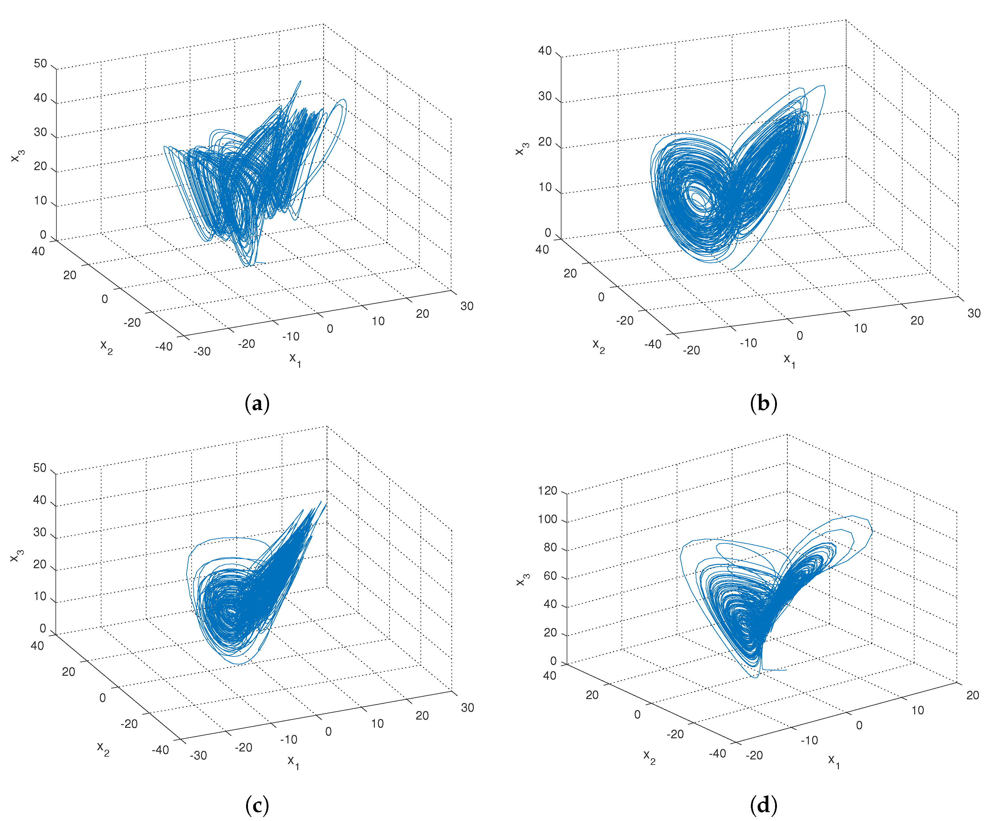
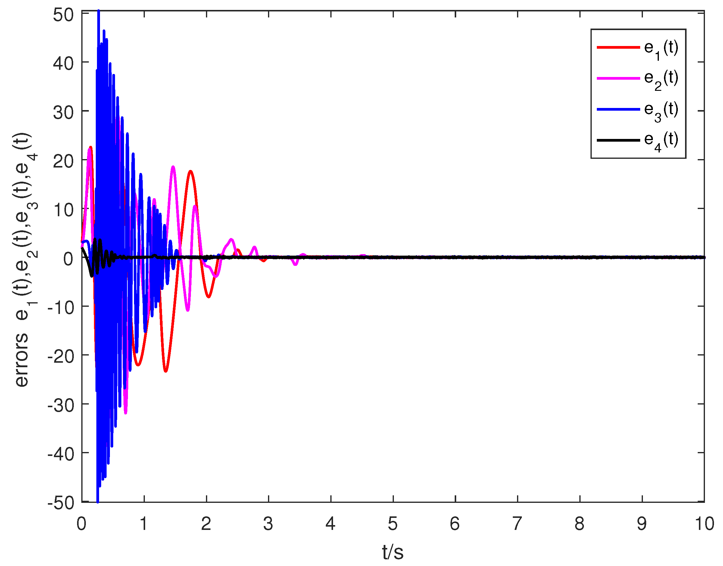
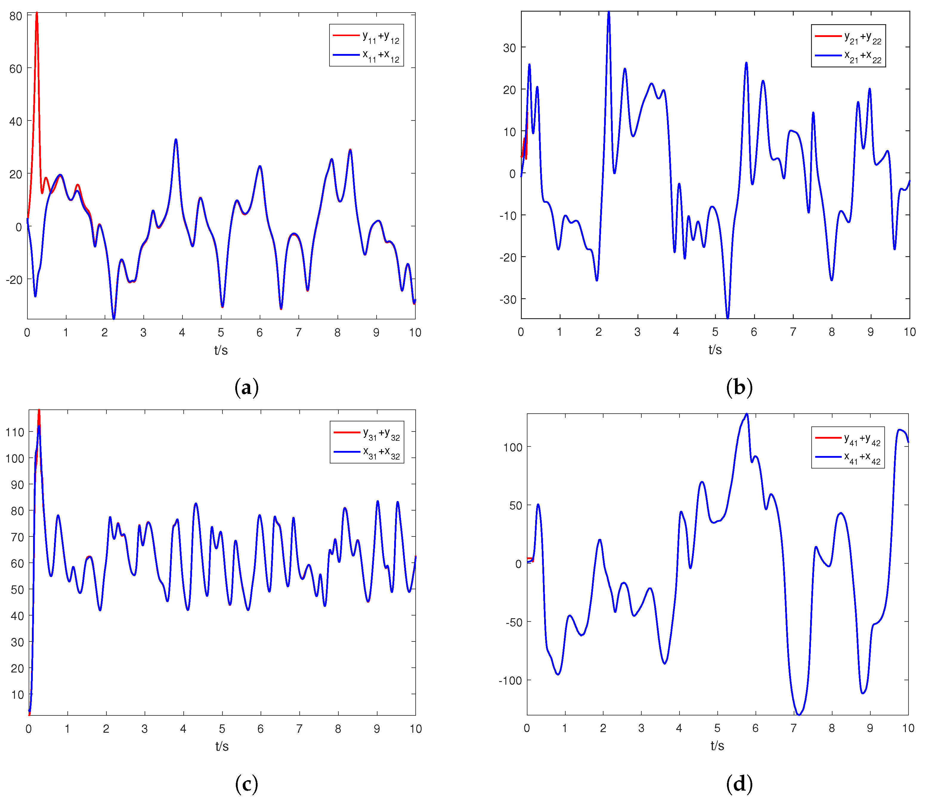
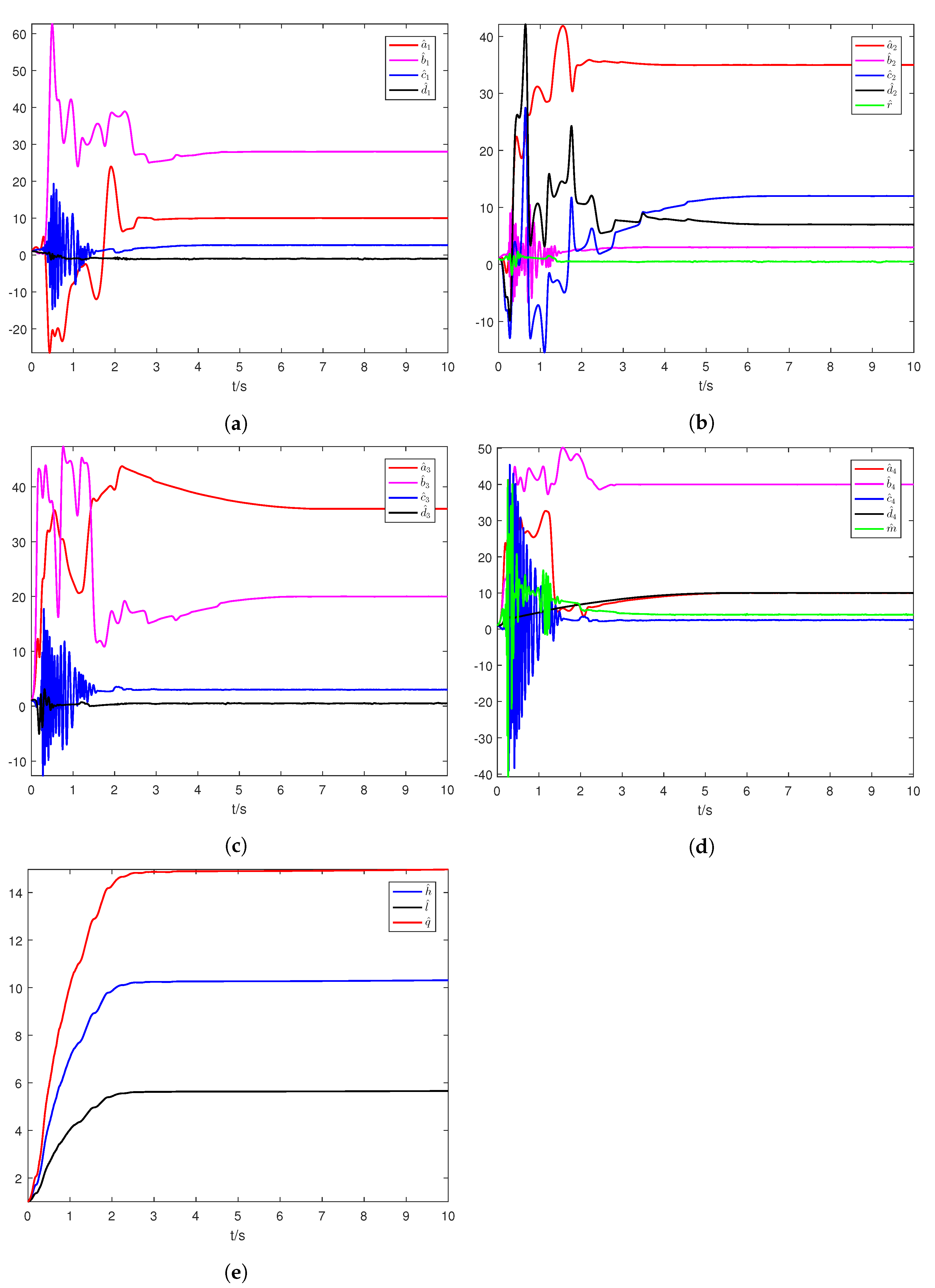
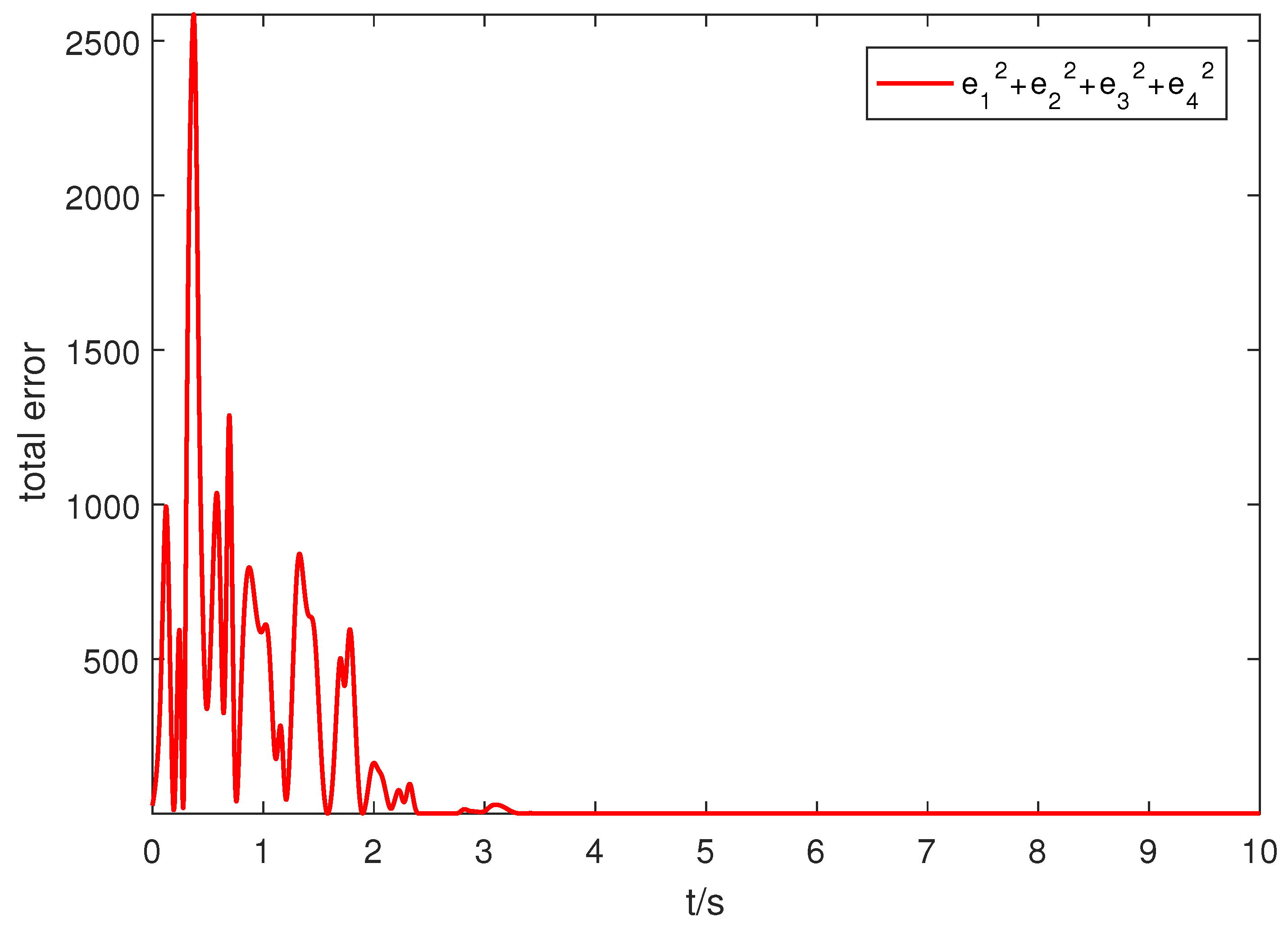
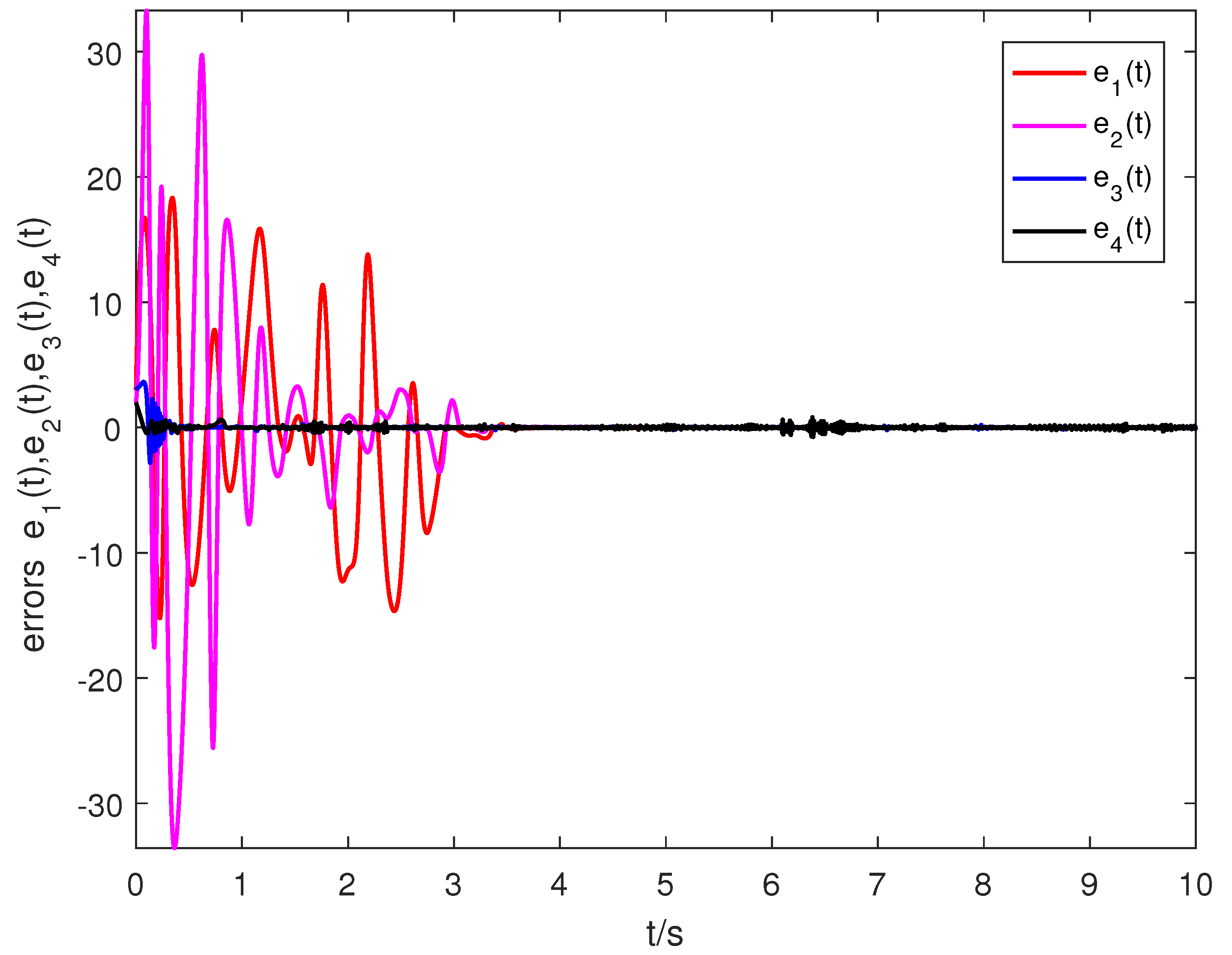
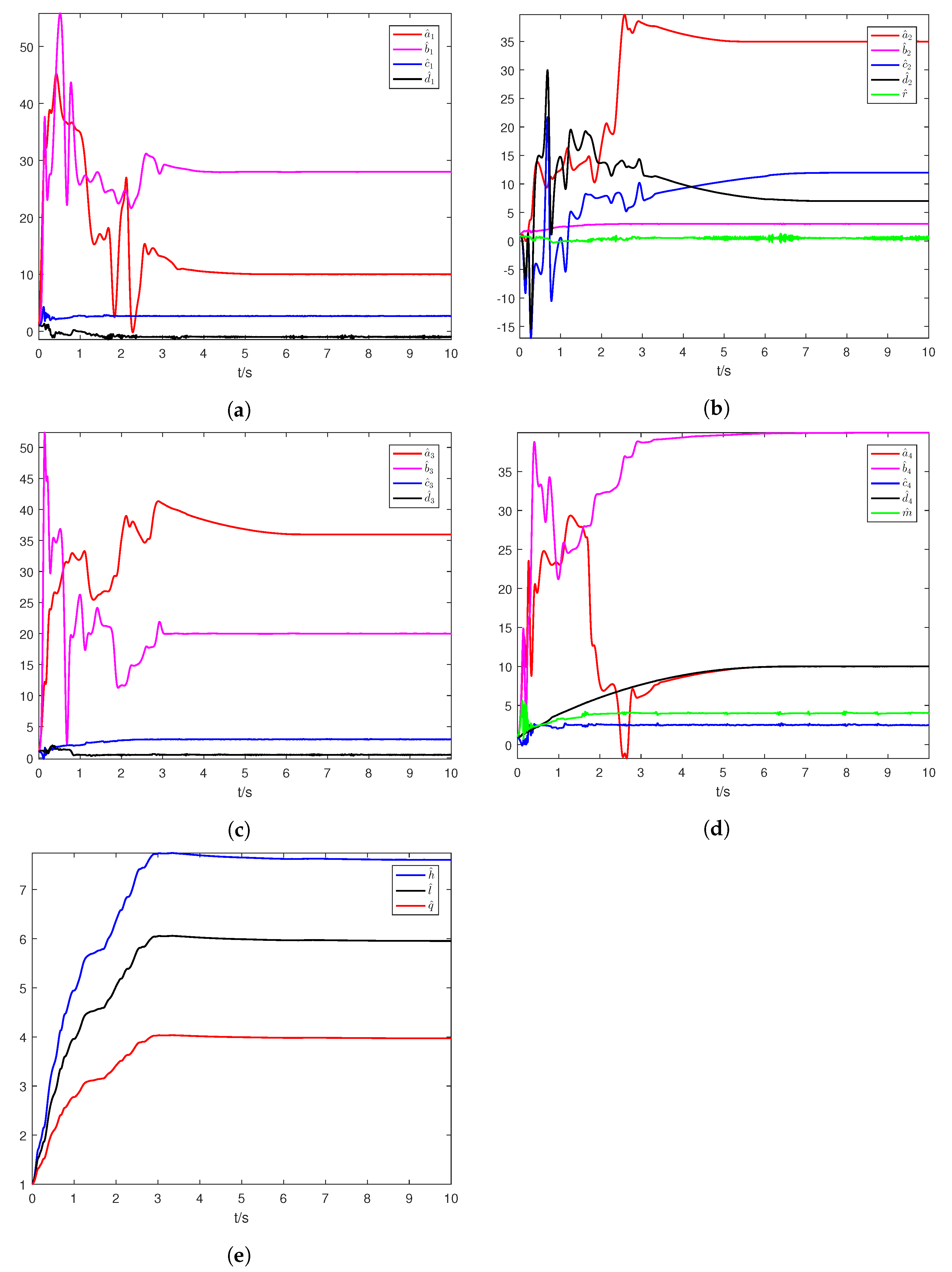
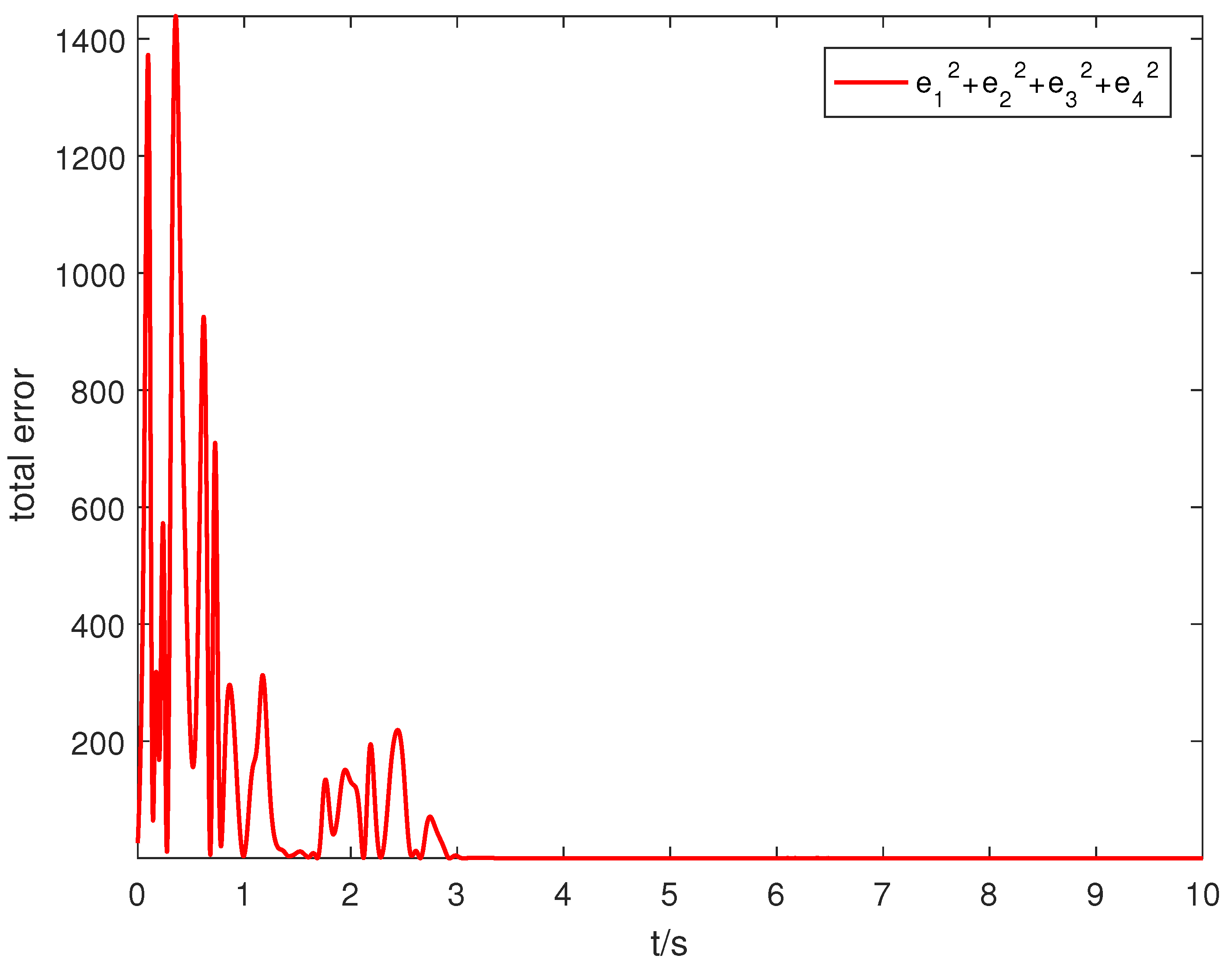
5. Numerical Simulation

Let the FO hyperchaotic Lorenz and Chen system under multiple SD be the drive systems

$$\begin{array}{cc}\hfill \left(\begin{array}{c}{}_0{D}_t^{\alpha }{x}_{11}\\ {}_0{D}_t^{\alpha }{x}_{21}\\ {}_0{D}_t^{\alpha }{x}_{31}\\ {}_0{D}_t^{\alpha }{x}_{41}\end{array}\right)& =\left(\begin{array}{cccc}{x}_{21}-x_{11}& 0& 0& 0\\ 0& x_{11}& 0& 0\\ 0& 0& -x_{31}& 0\\ 0& 0& 0& x_{41}\end{array}\right)\left(\begin{array}{c}{a}_1+\Delta a_1\\ b_1+\Delta b_1\\ c_1+\Delta c_1\\ d_1+\Delta d_1\end{array}\right)\hfill \\ & +\left(\begin{array}{c}{x}_{41}+\Delta f_{11}\\ -x_{11}{x}_{31}-x_{21}+\Delta f_{21}\\ x_{11}{x}_{21}+\Delta f_{31}\\ -x_{21}{x}_{31}+\Delta f_{41}\end{array}\right)+\left(\begin{array}{c}{d}_{11}\\ d_{21}\\ d_{31}\\ d_{41}\end{array}\right).\hfill \end{array}$$

(51)

$$\begin{array}{cc}\hfill \left(\begin{array}{c}{}_0{D}_t^{\alpha }{x}_{12}\\ {}_0{D}_t^{\alpha }{x}_{22}\\ {}_0{D}_t^{\alpha }{x}_{32}\\ {}_0{D}_t^{\alpha }{x}_{42}\end{array}\right)& =\left(\begin{array}{ccccc}{x}_{22}-x_{12}& 0& 0& 0& 0\\ 0& 0& x_{22}& x_{12}& 0\\ 0& -x_{32}& 0& 0& 0\\ 0& 0& 0& 0& x_{42}\end{array}\right)\left(\begin{array}{c}{a}_2+\Delta a_2\\ b_2+\Delta b_2\\ c_2+\Delta c_2\\ d_2+\Delta d_2\\ r+\Delta r\end{array}\right)\hfill \\ & +\left(\begin{array}{c}{x}_{42}+\Delta f_{12}\\ -x_{11}{x}_{32}+\Delta f_{22}\\ x_{12}{x}_{22}+\Delta f_{32}\\ x_{22}{x}_{32}+\Delta f_{42}\end{array}\right)+\left(\begin{array}{c}{d}_{12}\\ d_{22}\\ d_{32}\\ d_{42}\end{array}\right).\hfill \end{array}$$

(52)

Let the FO hyper-chaotic Lü and Liu chaotic system under multiple SD and controller be the response systems

$$\begin{array}{cc}\hfill \left(\begin{array}{c}{}_0{D}_t^{\alpha }{y}_{11}\\ {}_0{D}_t^{\alpha }{y}_{21}\\ {}_0{D}_t^{\alpha }{y}_{31}\\ {}_0{D}_t^{\alpha }{y}_{41}\end{array}\right)& =\left(\begin{array}{cccc}{y}_{21}-y_{11}& 0& 0& 0\\ 0& y_{21}& 0& 0\\ 0& 0& -y_{31}& 0\\ 0& 0& 0& y_{41}\end{array}\right)\left(\begin{array}{c}{a}_3+\Delta a_3\\ b_3+\Delta b_3\\ c_3+\Delta c_3\\ d_3+\Delta d_3\end{array}\right)\hfill \\ & +\left(\begin{array}{c}{y}_{41}+\Delta g_{11}\\ -y_{11}{y}_{31}+\Delta g_{21}\\ y_{11}{y}_{21}+\Delta g_{31}\\ y_{11}{y}_{31}+\Delta g_{41}\end{array}\right)+\left(\begin{array}{c}{\mu }_{11}+u_{11}\\ {\mu }_{21}+u_{21}\\ {\mu }_{31}+u_{31}\\ {\mu }_{41}+u_{41}\end{array}\right).\hfill \end{array}$$

(53)

$$\begin{array}{cc}\hfill \left(\begin{array}{c}{}_0{D}_t^{\alpha }{y}_{12}\\ {}_0{D}_t^{\alpha }{y}_{22}\\ {}_0{D}_t^{\alpha }{y}_{32}\\ {}_0{D}_t^{\alpha }{y}_{42}\end{array}\right)& =\left(\begin{array}{ccccc}{y}_{22}-y_{12}& 0& 0& 0& 0\\ 0& y_{12}& 0& 0& 0\\ 0& 0& -y_{32}& 0& y_{12}^2\\ 0& 0& 0& -y_{12}& 0\end{array}\right)\left(\begin{array}{c}{a}_4+\Delta a_4\\ b_4+\Delta b_4\\ c_4+\Delta c_4\\ d_4+\Delta d_4\\ m+\Delta m\end{array}\right)\hfill \\ & +\left(\begin{array}{c}\Delta g_{12}\\ -y_{12}{y}_{32}+y_{42}+\Delta g_{22}\\ \Delta g_{32}\\ \Delta g_{42}\end{array}\right)+\left(\begin{array}{c}{\mu }_{12}+u_{12}\\ {\mu }_{22}+u_{22}\\ {\mu }_{32}+u_{32}\\ {\mu }_{42}+u_{42}\end{array}\right).\hfill \end{array}$$

(54)

The chosen parameters are $a_1=10,b_1=28,c_1=8/3,d_1=-1$, $a_2=35,b_2=3,c_2=12,d_2=7,r=0.5$, $a_3=36,b_3=20,c_3=3,d_3=0.5$, $a_4=10,b_4=40,c_4=2.5,d_4=10,m=4$. The initial values take as ${\mathit{x}}_1\left(0\right)=(2,-2,1,-1)$, ${\mathit{x}}_2\left(0\right)=(1,1,2,2)$, ${\mathit{y}}_1\left(0\right)=(-1,3,1,3)$, ${\mathit{y}}_2\left(0\right)=(2,1,2,1)$. The orders take as $\alpha =0.99$. The combination D-R systems are in hyper-chaotic state which are presented in Figure 1.

Remark 12.

The ranges of fractional order that make the FO hyper-chaotic Chen, Lorenz, L and Liu chaotic system appear hyper-chaotic are chose as $0.8\le \alpha <1$, $0.97\le \alpha <1$, $0.94\le \alpha \le 1$, $0.96\le \alpha \le 1$ respectively. If the drive-response systems are in hyper-chaotic, the influence of stochastic disturbances on the system can be better studied, and the effectiveness and robustness of the controller can be proved. It follows that the dynamic error has the same fractional-order as the drive and response systems that the fractional order α is chose as $0.97\le \alpha <1$ which can ensure that the all drive-response systems are hyper-chaotic. Thus, in the numerical simulation section, we also consider the $\alpha =0.97$ to validate the proposed method.

According to the above equations, we consider:

${\widehat{\mathit{\theta }}}_1={({\widehat{a}}_1,{\widehat{b}}_1,{\widehat{c}}_1,{\widehat{d}}_1)}^T$,	${\widehat{\mathit{\theta }}}_2={({\widehat{a}}_2,{\widehat{b}}_2,{\widehat{c}}_2,{\widehat{d}}_2,\widehat{r})}^T$,
${\widehat{\mathit{\vartheta }}}_1={({\widehat{a}}_3,{\widehat{b}}_3,{\widehat{c}}_3,{\widehat{d}}_3)}^T$,	${\widehat{\mathit{\vartheta }}}_2={({\widehat{a}}_4,{\widehat{b}}_4,{\widehat{c}}_4,{\widehat{d}}_4,\widehat{m})}^T$,

The uncertain terms $\Delta {\mathit{\theta }}_i$, $\Delta {\mathit{\vartheta }}_i$, $\Delta {\mathit{f}}_i\left({\mathit{x}}_i\left(t\right)\right)$, $\Delta {\mathit{g}}_i\left({\mathit{y}}_i\left(t\right)\right)$ and external disturbance ${\mathit{d}}_i\left({\mathit{x}}_i\left(t\right)\right)$, ${\mathit{\mu }}_i\left({\mathit{y}}_i\left(t\right)\right)$ for $i=1,2$ are demonstrated as:

$$\begin{array}{cc}\hfill & \Delta {\mathit{\theta }}_1={(0.2sin\left(t\right),0.2sin\left(0.2t\right),0.2sin\left(3t\right),0.2sin\left(0.4t\right))}^T,\hfill \\ & \Delta {\mathit{\theta }}_2={(0.2sin\left(5t\right),0.2sin\left(0.6t\right),0.2sin\left(0.8t\right),0.2sin\left(2t\right),0.2sin\left(10t\right))}^T,\hfill \\ & \Delta {\mathit{\vartheta }}_1={(0.2sin\left(t\right),0.2sin\left(2t\right),0.2sin\left(3t\right),0.2sin\left(4t\right))}^T,\hfill \\ & \Delta {\mathit{\vartheta }}_2={(0.2sin\left(0.5t\right),0.2sin\left(6t\right),0.2sin\left(t\right),0.2sin\left(0.2t\right),0.2sin\left(3t\right))}^T,\hfill \\ & {\mathit{d}}_1\left({\mathit{x}}_1\left(t\right)\right)={(-0.1cos\left(t\right),-0.2cos\left(2t\right),0.3sin\left(3t\right),0.4sin\left(4t\right))}^T,\hfill \\ & {\mathit{d}}_2\left({\mathit{x}}_2\left(t\right)\right)={(-0.1sin\left(t\right),-0.2sin\left(2t\right),0.3cos\left(3t\right),0.4cos\left(4t\right))}^T,\hfill \\ & {\mathit{\mu }}_1\left({\mathit{y}}_1\left(t\right)\right)={(0.1cos\left(5t\right),0.2cos\left(6t\right),0.3sin\left(7t\right),0.4sin\left(8t\right))}^T,\hfill \\ & {\mathit{\mu }}_2\left({\mathit{y}}_2\left(t\right)\right)={(0.1sin\left(5t\right),0.2sin\left(6t\right),0.3cos\left(7t\right),0.4cos\left(8t\right))}^T,\hfill \\ & \Delta {\mathit{f}}_i\left({\mathit{x}}_i\left(t\right)\right)={(0.1cos\left(x_{1i}\right),0.2cos\left(x_{2i}\right),0.3cos\left(x_{3i}\right),0.4cos\left(x_{4i}\right))}^T,\hfill \\ & \Delta {\mathit{g}}_i\left({\mathit{y}}_i\left(t\right)\right)={(0.1sin\left(y_{1i}\right),0.2sin\left(y_{2i}\right),0.3sin\left(y_{3i}\right),0.4sin\left(y_{4i}\right))}^T,\hfill \end{array}$$

(55)

where $i=1,2$. It follows from (30), (31) and (34) that the error dynamics and the updating rules of unknown parameters are expressed as:

$$\begin{array}{cc}\hfill {}_0{D}_t^{\alpha }& e_1\left(t\right)=\left[-({\widehat{a}}_3-a_3)-0.2sin\left(t\right)\right](y_{21}-y_{11})-\left[({\widehat{a}}_4-a_4)+0.2sin\left(0.5t\right)\right](y_{22}-y_{12})\hfill \\ & +\left[({\widehat{a}}_1-a_1)-0.2sin\left(t\right)\right](x_{21}-x_{11})+\left[({\widehat{a}}_2-a_2)-0.2sin\left(5t\right)\right](x_{22}-x_{12})\hfill \\ & +\left[0.1sin\left(y_{11}\right)+0.1sin\left(y_{12}\right)-0.1cos\left(x_{11}\right)-0.1cos\left(x_{12}\right)\right]\hfill \\ & +\left[0.1cos\left(5t\right)+0.1sin\left(5t\right)+0.1cos\left(t\right)+0.1sin\left(t\right)\right]-\frac{1}{\gamma }sgn\left(e_1\left(t\right)\right){\parallel \mathit{e}\left(t\right)\parallel }^{\xi }\hfill \\ & -\varsigma (\parallel \widehat{{\mathit{\theta }}_1}\parallel +\parallel \widehat{{\mathit{\theta }}_2}\parallel +\parallel \widehat{{\mathit{\vartheta }}_1}\parallel +\parallel \widehat{{\mathit{\vartheta }}_2}\parallel +{\rho }_1|\widehat{h}|+{\rho }_2|\widehat{l}|+{\rho }_3|\widehat{q}|+{\delta }_1+{\delta }_2+{\delta }_3\hfill \\ & +{\delta }_4+{\rho }_1{h}^{*}+{\rho }_2{l}^{*}+{\rho }_3{q}^{*})(\frac{s_1}{{\gamma \parallel \mathit{s}\parallel }^2})-(\widehat{h}+\widehat{l}+\widehat{q})sgn\left(s_1\right)-\frac{k}{\gamma }.\hfill \end{array}$$

$$\begin{array}{cc}\hfill {}_0{D}_t^{\alpha }& e_2\left(t\right)=\left[-({\widehat{b}}_3-b_3)+0.2sin\left(2t\right)\right]y_{21}-\left[({\widehat{b}}_4-b_4)-0.2sin\left(6t\right)\right]y_{12}\hfill \\ & +\left[({\widehat{b}}_1-b_1)-0.2sin\left(0.2t\right)\right]x_{11}+\left[({\widehat{c}}_2-c_2)-0.2sin\left(0.6\right)\right]x_{22}\hfill \\ & +\left[({\widehat{d}}_2-d_2)-0.2sin\left(0.8\right)\right]x_{12}+\left[0.2sin\left(y_{21}\right)+0.2sin\left(y_{22}\right)\right]\hfill \\ & \left[-0.2cos\left(x_{21}\right)-0.2cos\left(x_{22}\right)\right]+\left[0.2cos\left(6t\right)+0.2sin\left(6t\right)+0.2cos\left(2t\right)+0.2sin\left(2t\right)\right]\hfill \\ & -\frac{1}{\gamma }sgn\left(e_2\left(t\right)\right){\parallel \mathit{e}\left(t\right)\parallel }^{\xi }-\varsigma (\parallel \widehat{{\mathit{\theta }}_1}\parallel +\parallel \widehat{{\mathit{\theta }}_2}\parallel +\parallel \widehat{{\mathit{\vartheta }}_1}\parallel +\parallel \widehat{{\mathit{\vartheta }}_2}\parallel +{\rho }_1|\widehat{h}|+{\rho }_2|\widehat{l}|+{\rho }_3|\widehat{q}|+{\delta }_1\hfill \\ & +{\delta }_2+{\delta }_3+{\delta }_4+{\rho }_1{h}^{*}+{\rho }_2{l}^{*}+{\rho }_3{q}^{*})(\frac{s_2}{{\gamma \parallel \mathit{s}\parallel }^2})-(\widehat{h}+\widehat{l}+\widehat{q})sgn\left(s_2\right)-\frac{k}{\gamma }.\hfill \end{array}$$

$$\begin{array}{cc}\hfill {}_0{D}_t^{\alpha }& e_3\left(t\right)=\left[({\widehat{c}}_3-c_3)-0.2sin\left(3t\right)\right]y_{31}+\left[({\widehat{c}}_4-c_4)-0.2sin\left(t\right)\right]y_{32}\hfill \\ & -\left[(\widehat{m}-m)-0.2sin\left(3t\right)\right]y_{12}^2-\left[({\widehat{c}}_1-c_1)-0.2sin\left(3t\right)\right]x_{31}\hfill \\ & -\left[({\widehat{b}}_2-b_2)-0.2sin\left(0.6t\right)\right]x_{32}+\left[0.3sin\left(y_{31}\right)+0.3sin\left(y_{32}\right)-0.3cos\left(x_{31}\right)-0.3cos\left(x_{32}\right)\right]\hfill \\ & +\left[0.3cos\left(7t\right)+0.3sin\left(7t\right)-0.3cos\left(3t\right)-0.3sin\left(3t\right)\right]-\frac{1}{\gamma }sgn\left(e_3\left(t\right)\right){\parallel \mathit{e}\left(t\right)\parallel }^{\xi }\hfill \\ & -\varsigma (\parallel \widehat{{\mathit{\theta }}_1}\parallel +\parallel \widehat{{\mathit{\theta }}_2}\parallel +\parallel \widehat{{\mathit{\vartheta }}_1}\parallel +\parallel \widehat{{\mathit{\vartheta }}_2}\parallel +{\rho }_1|\widehat{h}|+{\rho }_2|\widehat{l}|+{\rho }_3|\widehat{q}|+{\delta }_1+{\delta }_2\hfill \\ & +{\delta }_3+{\delta }_4+{\rho }_1{h}^{*}+{\rho }_2{l}^{*}+{\rho }_3{q}^{*})(\frac{s_3}{{\gamma \parallel \mathit{s}\parallel }^2})-(\widehat{h}+\widehat{l}+\widehat{q})sgn\left(s_3\right)-\frac{k}{\gamma }.\hfill \end{array}$$

$$\begin{array}{cc}\hfill {}_0{D}_t^{\alpha }& e_4\left(t\right)=\left[-({\widehat{d}}_3-d_3)+0.2sin\left(4t\right)\right]y_{41}+\left[({\widehat{d}}_4-d_4)+0.2sin\left(0.2t\right)\right]y_{12}\hfill \\ & +\left[({\widehat{d}}_1-d_1)-0.2sin\left(0.4t\right)\right]x_{41}+\left[(\widehat{r}-r)-0.2sin\left(10t\right)\right]x_{42}\hfill \\ & +\left[0.4sin\left(y_{41}\right)+0.4sin\left(y_{42}\right)-0.4cos\left(x_{41}\right)-0.4cos\left(x_{42}\right)\right]\hfill \\ & +\left[0.4cos\left(8t\right)+0.4sin\left(8t\right)-0.4cos\left(4t\right)-0.4sin\left(4t\right)\right]\hfill \\ & -\frac{1}{\gamma }sgn\left(e_4\left(t\right)\right){\parallel \mathit{e}\left(t\right)\parallel }^{\xi }-\varsigma (\parallel \widehat{{\mathit{\theta }}_1}\parallel +\parallel \widehat{{\mathit{\theta }}_2}\parallel +\parallel \widehat{{\mathit{\vartheta }}_1}\parallel +\parallel \widehat{{\mathit{\vartheta }}_2}\parallel \hfill \\ & +{\rho }_1|\widehat{h}|+{\rho }_2|\widehat{l}|+{\rho }_3|\widehat{q}|+{\delta }_1+{\delta }_2+{\delta }_3+{\delta }_4+{\rho }_1{h}^{*}+{\rho }_2{l}^{*}+{\rho }_3{q}^{*})(\frac{s_4}{{\gamma \parallel \mathit{s}\parallel }^2})\hfill \\ & -(\widehat{h}+\widehat{l}+\widehat{q})sgn\left(s_4\right)-\frac{k}{\gamma }.\hfill \end{array}$$

$$\begin{array}{cc}& {}_0{D}_t^{\mathit{\alpha }}\widetilde{{\mathit{\theta }}_1}=\gamma \left[{((x_{11}-x_{21})s_1,-x_{11}{s}_2,x_{31}{s}_3,-x_{41}{s}_4)}^T\right],\hfill \\ & {}_0{D}_t^{\mathit{\alpha }}\widetilde{{\mathit{\theta }}_2}=\gamma \left[{((x_{12}-x_{22})s_1,x_{32}{s}_3,-x_{22}{s}_2,-x_{12}{s}_2,-x_{42}{s}_4)}^T\right],\hfill \\ & {}_0{D}_t^{\mathit{\alpha }}\widetilde{{\mathit{\vartheta }}_1}=\gamma \left[{((y_{21}-y_{11})s_1,y_{21}{s}_2,-y_{31}{s}_3,y_{41}{s}_4)}^T\right],\hfill \\ & {}_0{D}_t^{\mathit{\alpha }}\widetilde{{\mathit{\vartheta }}_2}=\gamma \left[{((y_{22}-y_{12})s_1,y_{12}{s}_2,-y_{32}{s}_3,-y_{12}{s}_4,y_{12}^2{s}_3)}^T\right],\hfill \\ & {}_0{D}_t^{\mathit{\alpha }}\tilde{h}=\gamma {\rho }_1\sqrt{(s_1^2+s_2^2+s_3^2+s_4^2)},\hfill \\ & {}_0{D}_t^{\mathit{\alpha }}\tilde{l}=\gamma {\rho }_2\sqrt{(s_1^2+s_2^2+s_3^2+s_4^2)},\hfill \\ & {}_0{D}_t^{\mathit{\alpha }}\tilde{q}=\gamma {\rho }_3\sqrt{(s_1^2+s_2^2+s_3^2+s_4^2)},\hfill \end{array}$$

In the numerical simulation section, the method we adopted for the fractional order chaotic system is the Adams–Bashforth–Moulton type predictor-corrector scheme [25]. We use the Matlab software (R2016a) to solve them. For the simulation procedure, The initial values of D-R systems take as ${\mathit{x}}_1\left(0\right)=(2,-2,1,-1)$, ${\mathit{x}}_2\left(0\right)=(1,1,2,2)$, ${\mathit{y}}_1\left(0\right)=(-1,3,1,3)$, ${\mathit{y}}_2\left(0\right)=(2,1,2,1)$. The orders take as $\alpha =0.99$. The time step is 0.003. The number of iterations is 3000. The initial conditions of parameters estimation are $(a_1\left(0\right),b_1\left(0\right),c_1\left(0\right),d_1\left(0\right))=(1,1,1,1)$, $(a_2\left(0\right),b_2\left(0\right),c_2\left(0\right),d_2\left(0\right),r\left(0\right))=(1,1,1,1,1)$, $(a_3\left(0\right),b_3\left(0\right),c_3\left(0\right),d_3\left(0\right))=(1,1,1,1)$, $h\left(0\right),l\left(0\right),q\left(0\right)=(1,1,1)$, $(a_4\left(0\right),b_4\left(0\right),c_4\left(0\right),d_4\left(0\right),m\left(0\right))=(1,1,1,1,1)$. The constants are chosen as $\gamma =1,{\delta }_1=100,{\delta }_2=100,{\delta }_3=100,{\delta }_4=100,h^{*}=50,l^{*}=50,q^{*}=50,{\rho }_1=0.1$, ${\rho }_2=0.2,{\rho }_3=0.3,\xi =0.5,\varsigma =3,k=4.$ For $\alpha =0.99$, the trajectories about the error variables $e_i\left(t\right),(i=1,2,3,4)$ are depicted in Figure 2 and the synchronization for the state trajectories of drive systems (18), (19) and response system (20), (21) are drawn in Figure 3. The trajectories of estimations $\widehat{{\mathit{\theta }}_i}$, $\widehat{{\mathit{\vartheta }}_i},(i=1,2)$, $\widehat{h}$, $\widehat{l}$, $\widehat{q}$ are depicted in Figure 4. Finally, in order to prove that the error variables converge completely to zero for $\alpha =0.99$, the sum of squares of all errors ($e_1^2+e_2^2+e_3^2+e_4^2$) is conducted as shown in Figure 5. For $\alpha =0.97$, the trajectories about the error variables $e_i\left(t\right),(i=1,2,3,4)$ are drawn in Figure 6 and the trajectories of estimations $\widehat{{\mathit{\theta }}_i}$, $\widehat{{\mathit{\vartheta }}_i},(i=1,2)$, $\widehat{h}$, $\widehat{l}$, $\widehat{q}$ are drawn in Figure 7. Finally, in order to prove that the error variables converge completely to zero for $\alpha =0.97$, the sum of squares of all errors ($e_1^2+e_2^2+e_3^2+e_4^2$) is conducted as shown in Figure 8. It all demonstrates that the the error does converge completely to zero. Therefore, this controller and the updated rules of the parameters are effective.

Remark 13.

In the numerical simulation section, the fractional order (FO) hyper-chaotic Lorenz and Chen system are the drive systems. The fractional order hyper-chaotic L$\ddot{u}$ and Liu chaotic system are the response systems. The equilibrium positions of drive-response systems are as follows. The FO hyper-chaotic Lorenz system $E_1=(0,0,0,0)$, $E_2=(-1.17,-21.63,9.46,204.60),$ $E_3=(1.17,21.63,9.46,-204.60)$. The FO hyper-chaotic Chen system $E_1=(0,0,0,0)$. The FO hyper-chaotic L$\ddot{u}$ system $E_1=(0,0,0,0)$, $E_2=(7.75,9.30,3.60,55.77)$, $E_3=(-7.75,-9.30,3.60,-55.77)$ The FO hyper-chaotic Liu system $E_1=(0,0,0,0)$. Now, there is a question worth thinking about, which is whether the proposed method is still valid for systems with a large number of equilibria. Thus, the numerical simulation for the systems with three equilibrium positions are conducted. They are the FO Lorenz system, the FO L$\ddot{u}$ system, the FO Genesio–Tesi system and the FO Arneodo system. The results are also valid. In fact, the adaptive combination controller has nothing to do with the number of equilibrium positions. In addition to the numerical simulation results we have obtained, there are also some references [45,46,49,61]. From the numerical simulation section of this literature, the choice of the drive-response system is arbitrary. Thus, the proposed method is still valid for systems with a large number of equilibria.

A comparison analysis between the proposed finite-time combination–combination (C-C) synchronization (FTCCS) scheme and the earlier published work is as follows. In Ref. [62], the author applied the adaptive control method to achieve C-C synchronization among four identical hyper-chaotic systems where it noted that the synchronization states happened at $t=5$ (approx). In Ref. [61], the author used the sliding mode control scheme to address multiple chaotic systems with unknown parameters and disturbances in which the synchronization happened at $t=5$ (approx). Besides, in Ref. [63], the author solved a new type of C-C synchronization for four identical or different chaotic systems via adaptive control, where the desired synchronization happened at $t=5.5$ (approx). The combination synchronization of FO non-autonomous chaotic systems with different dimensions adopting a scaling matrix is studied in Ref. [64], where the error synchronization happened at $t=6$ (approx). Furthermore, the phase synchronization of FO complex chaotic systems with different structures is discussed in Ref. [65]; in the process of C-C synchronization, the desired synchronization happened at $t=4.5$ (approx). The nonsingular terminal sliding mode control to achieve the finite-time synchronization between two complex-variable chaotic systems with unknown parameters is adopted in Ref. [66]; here it has been found that the synchronization error converges to zero at $t=10$ (approx). In addition to the above studies, we have investigated the FTCCS scheme among fractional order (FO) chaotic systems under multiple stochastic disturbances (SD), utilizing the nonsingular terminal sliding mode control (NTSMC) technique in which it has been recorded that the synchronization occurs at $t=3.1$ (approx) as depicted in Figure 5. Therefore, comparing the synchronization times discussed above with those obtained by our proposed scheme, our method is dominant. This also illustrates the vitality and effectivity of the considered methodology.

Remark 14.

After calculation, the finite synchronization time satisfies $T_1\le 5.71$, $T_2\le 7.34$ theoretically. Thus, we have $T\le T_1+T_2=13.05$. Comparing the numerical simulation results, we can see that our control scheme is effective.

Remark 15.

The dynamic error has the same fractional-order as the D-R systems in our paper. It is worth considering that the non-integer order in the derivative of error is different from the D-R. If we only consider this situation, there are many papers that have discussed it. In Ref. [67], the author proposed a modified adaptive sliding-mode control technique to investigate the reduced-order and increased-order synchronization. Ouannas et al. [68] investigated the inverse full state hybrid function projective synchronization (IFSHFPS) of non-identical systems characterized by different dimensions and different orders. Furthermore, the hybrid projective synchronization of different dimensional fractional order chaotic systems with time delay and different orders is discussed by [69]. More research results can be found in Refs. [70,71,72]. All the above literature about the non-integer order in the derivative of error is different from the drive-response systems. Our next step will consider this situation.

6. Conclusions

In this article, the FTCCS of FO chaotic systems among four systems with different structures and unknown parameters is solved. The most important point is that the conditions we consider are under multiple stochastic disturbances. Our thought for this topic is that under the action of the finite-time Lyapunov theory and the nonsingular terminal sliding mode control technique, we deduced a new FO sliding surface, adaptive combination controller and some parameter updating laws, which can achieve the combination–combination synchronization of systems under multiple stochastic disturbances in finite time. The unknown parameters are identified precisely. Moreover, the combination drive systems and combination response systems that we introduced are very general. The expression of the synchronization error system makes many synchronization methods, such as chaos control, complete synchronization, projection synchronization, anti-synchronization and so forth, become special cases of combination–combination synchronization. From the numerical simulation results, it is obvious that the error variables of the D-R systems quickly converge to the origin point in the given time. Therefore, this controller and the updated parameter laws are effective. Next, for the multiple stochastic disturbances, we will study the fractional order multi switching synchronization of eight chaotic systems with time-delay in which the systems’ parameters are still unknown.

References

1. Ping, Z.; Peng, Z. Drive-response synchronization for chaotic systems. J. Chong Qing Univ. 2002, 25, 77–79. [Google Scholar]
2. Yu, J.; Hu, C.; Jiang, H. Projective synchronization for fractional neural networks. Neural Netw. 2014, 49, 87–95. [Google Scholar] [CrossRef] [PubMed]
3. Shao, K.; Guo, H.; Han, F. Finite-time projective synchronization of fractional-order chaotic systems via soft variable structure control. J. Mech. Sci. Technol. 2020, 34, 369–376. [Google Scholar] [CrossRef]
4. Qin, X.; Li, S.; Liu, H. Adaptive fuzzy synchronization of uncertain fractional-order chaotic systems with different structures and time-delays. Adv. Diff. Equ. 2019, 2019, 174. [Google Scholar] [CrossRef]
5. Bouzeriba, A.; Boulkroune, A.; Bouden, T. Fuzzy adaptive synchronization of a class of fractional-order chaotic systems. In Proceedings of the 2015 3rd International Conference on Control, Engineering & Information Technology (CEIT), Tlemcen, Algeria, 25–27 May 2015; Volume 7, pp. 1–16. [Google Scholar]
6. Liu, Y.J.; Gong, M.; Tong, S.; Chen, C.P.; Li, D.J. Adaptive fuzzy output feedback control for a class of nonlinear systems with full state constraints. IEEE Trans. Fuzzy. Syst. 2018, 26, 2607–2617. [Google Scholar] [CrossRef]
7. Ha, S.; Chen, L.; Liu, H. Command filtered adaptive neural network synchronization control of fractional-order chaotic systems subject to unknown dead zones. J. Frankl. Inst. 2021, 358, 3376–3402. [Google Scholar] [CrossRef]
8. Zeng, H.B.; Teo, K.L.; He, Y.; Xu, H.; Wang, W. Sampled-data synchronization control for chaotic neural networks subject to actuator saturation. Neurocomputing 2017, 185, 1656–1667. [Google Scholar] [CrossRef]
9. Wang, J.; Xu, C. Stochastic feedback coupling synchronization of networked harmonic oscillators. Automatica 2018, 87, 404–411. [Google Scholar] [CrossRef]
10. Li, H.L.; Jiang, Y.L.; Wang, Z.; Zhang, L.; Teng, Z. Parameter identification and adaptive-impulsive synchronization of uncertain complex networks with nonidentical topological structures. Optik-Int. J. Light Electron. Opt. 2015, 126, 5771–5776. [Google Scholar] [CrossRef]
11. Li, X.F.; Chu, Y.D.; Leung, A.Y.; Zhang, H. Synchronization of uncertain chaotic systems via complete-adaptive-impulsive controls. Chaos Solitons Fractals 2017, 100, 24–30. [Google Scholar] [CrossRef]
12. Kocamaz, U.E.; Cevher, B.; Uyaroğlu, Y. Control and synchronization of chaos with sliding mode control based on cubic reaching rule. Chaos Solitons Fractals 2017, 105, 92–98. [Google Scholar] [CrossRef]
13. Vaidyanathan, S. Anti-synchronization of 3-cells cellular neural network attractors via integral sliding mode control. Int. J. PharmTech Res. 2016, 9, 193–205. [Google Scholar]
14. Li, X.; Zhao, X.S. The chaotic synchronization of fractional-order and integer-order in a class of financial systems. J. Sci. Teach. Coll. Univ. 2020, 40, 1–4. [Google Scholar]
15. Jing, W.; Guang, P. Design of a sliding mode controller for synchronization of fractional-order chaotic systems with different structures. J. Shanghai Jiaotong Univ. 2016, 50, 849–860. [Google Scholar]
16. Jiang, N. The adaptive control synchronization of hyper-chaos lorenz system and hyper-chaos Rössler system. J. Taiyuan Norm Univ. 2014, 13, 47–50. [Google Scholar]
17. Wei, X. Adaptive control and synchronization of Lü hyper-chaotic system. J. Honghe Univ. 2015, 13, 23–27. [Google Scholar]
18. Li, T.; Wang, Y.; Zhao, C. Synchronization of fractional chaotic systems based on a simple Lyapunov function. Adv. Diff. Equ. 2017, 2017, 304. [Google Scholar] [CrossRef] [Green Version]
19. Wei, Y.H.; Chen, Y.Q. Lyapunov functions for nabla discrete fractional order systems. ISA Trans. 2019, 88, 82–90. [Google Scholar] [CrossRef]
20. Tirandaz, H.; Tavakoli, H.R.; Ahmadnia, M. Modified projective synchronization of chaotic systems with noise disturbance, an active nonlinear control method. Int. J. Electr. Comput. Eng. 2017, 7, 3436–3445. [Google Scholar] [CrossRef] [Green Version]
21. Khan, A.; Jahanzaib, L.S. Synchronization on the adaptive sliding mode controller for fractional order complex chaotic systems with uncertainty and disturbances. Int. J. Dyn. Control 2019, 7, 1419–1433. [Google Scholar] [CrossRef]
22. Luo, R.; Su, H.; Zeng, Y. Synchronization of uncertain fractional-order chaotic systems via a novel adaptive controller. Chin. J. Phys. 2017, 55, 342–349. [Google Scholar] [CrossRef]
23. Kekha Javan, A.A.; Shoeibi, A.; Zare, A.; Hosseini Izadi, N.; Jafari, M.; Alizadehsani, R.; Moridian, P.; Mosavi, A.; Acharya, U.R.; Nahavandi, S. Design of Adaptive-Robust Controller for Multi-State Synchronization of Chaotic Systems with Unknown and Time-Varying Delays and Its Application in Secure Communication. Sensors 2021, 21, 254. [Google Scholar] [CrossRef] [PubMed]
24. Khan, A.; Chaudhary, H. Hybrid projective combination-combination synchronization in non-identical hyperchaotic systems using adaptive control. Arab. J. Math. 2020, 9, 597–611. [Google Scholar] [CrossRef] [Green Version]
25. Petras, I. Fractional-Order Nonlinear Systems, Modeling, Analysis and Simulation; Higher Education Press: Beijing, China, 2011. [Google Scholar]
26. Mirrezapour, S.Z.; Zare, A.; Hallaji, M. A new fractional sliding mode controller based on nonlinear fractional-order proportional integral derivative controller structure to synchronize fractional-order chaotic systems with uncertainty and disturbances. J. Vib. Control 2021, 1–13. [Google Scholar] [CrossRef]
27. Zhang, R.; Yang, S. Robust chaos synchronization of fractional-order chaotic systems with unknown parameters and uncertain perturbations. Nonlinear Dyn. 2012, 69, 983–992. [Google Scholar] [CrossRef]
28. Ma, S.J.; Shen, Q.; Jing, H. Modified projective synchronization of stochastic fractional order chaotic systems with uncertain parameters. Nonlinear Dyn. 2013, 73, 93–100. [Google Scholar] [CrossRef]
29. Wang, Q.; Qi, D.L. Synchronization for fractional order chaotic systems with uncertain parameters. Int. J. Control Autom. Syst. 2016, 14, 211–216. [Google Scholar] [CrossRef]
30. Nian, F.; Liu, X.; Zhang, Y. Sliding mode synchronization of fractional-order complex chaotic system with parametric and external disturbances. Chaos Solitons Fractals 2018, 116, 22–28. [Google Scholar] [CrossRef]
31. Zhang, X.; Zhang, X.; Li, D.; Yang, D. Adaptive Synchronization for a Class of Fractional Order Time-delay Uncertain Chaotic Systems via Fuzzy Fractional Order Neural Network. Int. J. Control Autom. Syst. 2019, 17, 1209–1220. [Google Scholar] [CrossRef]
32. Deepika, D.; Sandeep, K.; Shiv, N. Uncertainty and disturbance estimator based robust synchronization for a class of uncertain fractional chaotic system via fractional order sliding mode control. Chaos Solitons Fractals 2018, 115, 196–203. [Google Scholar] [CrossRef]
33. Bhat, S.; Bernstein, D. Finite-time stability of homo-gencous systems. In Proceedings of the ACC, Albuquergue, NM, USA, 6 December 1997; pp. 2513–2514. [Google Scholar]
34. Velmurugan, G.; Rakkiyappan, R.; Cao, J. Finite-time synchronization of fractional-order memristor-based neural networks with time delays. Neural Netw. 2016, 73, 36–46. [Google Scholar] [CrossRef] [PubMed]
35. Lin, M.L.; Yuan, Z.Z.; Cai, J.P. Finite-time synchronization between two different chaotic systems with uncertainties. J. Fujian Univ. Technol. 2019, 17, 77–82. [Google Scholar]
36. Lan, T.L.; Wang, Y.J. Finite-time synchronization and parameters identification of a uncertain critical chaotic system. Math. Pract. Theory 2018, 48, 105–112. [Google Scholar]
37. Rashidnejad, Z.; Karimaghaee, P. Synchronization of a class of uncertain chaotic systems utilizing a new finite-time fractional adaptive sliding mode control. Chaos Solitons Fractals 2020, 5, 100042. [Google Scholar] [CrossRef]
38. Luo, Y.; Yao, Y. Finite-time synchronization of uncertain complex dynamic networks with time-varying delay. Adv. Diff. Equ. 2020, 2020, 32. [Google Scholar] [CrossRef]
39. Mishra, A.K.; Das, S.; Yadav, V.K. Finite-time synchronization of multi-scroll chaotic systems with sigmoid non-linearity and uncertain terms. Chin. J. Phys. 2020, 75, 235–245. [Google Scholar] [CrossRef]
40. Sweetha, S.; Sakthivel, R.; Harshavarthini, S. Finite-time synchronization of nonlinear fractional chaotic systems with stochastic actuator faults. Chaos Solitons Fractals 2020, 142, 110312. [Google Scholar] [CrossRef]
41. Li, H.L.; Cao, J.; Jiang, H.; Alsaedi, A. Finite-time synchronization and parameter identification of uncertain fractional-order complex networks. Phys. A Stat. Mech. Appl. 2019, 533, 122027. [Google Scholar] [CrossRef]
42. Sun, J.; Shen, Y.; Wang, X.; Chen, J. Finite-time combination-combination synchronization of four different chaotic systems with unknown parameters via sliding mode control. Nonlinear Dyn. 2014, 76, 383–397. [Google Scholar] [CrossRef]
43. Luo, R.Z.; Wang, Y.L.; Deng, S.C. Combination synchronization of three classic chaotic systems using active back-stepping design. Chaos Interdiscip. J. Nonlinear Sci. 2011, 21, 043114. [Google Scholar]
44. Luo, R.Z.; Wang, Y.L. Finite-time stochastic combination synchronization of three different chaotic systems and its application in secure communication. Chaos Interdiscip. J. Nonlinear Sci. 2012, 22, 821–824. [Google Scholar]
45. Khan, A.; Khattar, D.; Prajapati, N. Dual combination combination multi switching synchronization of eight chaotic systems. Chin. J. Phys. 2017, 55, 1209–1218. [Google Scholar] [CrossRef] [Green Version]
46. Ahmad, I.; Shafiq, M.; Al-Sawalha, M.M. Globally exponential multi switching-combination synchronization control of chaotic systems for secure communications. Chin. J. Phys. 2018, 56, 974–987. [Google Scholar] [CrossRef]
47. Khan, A.; Nigar, U. Adaptive hybrid complex projective combination-combination synchronization in non-identical hyper-chaotic complex systems. Int. J. Dynam. Control 2019, 7, 1404–1418. [Google Scholar] [CrossRef]
48. Vincent, U.E.; Saseyi, A.O.; Mcclintock, P. Multi-switching combination synchronization of chaotic systems. Nonlinear Dyn. 2015, 80, 845–854. [Google Scholar] [CrossRef] [Green Version]
49. Sun, J.; Cui, G.; Wang, Y.; Shen, Y. Combination complex synchronization of three chaotic complex systems. Nonlinear Dyn. 2015, 79, 953–965. [Google Scholar] [CrossRef]
50. Khan, A.; Budhraja, M.; Ibraheem, A. Combination-combination synchronisation of time-delay chaotic systems for unknown parameters with uncertainties and external disturbances. Pramana 2018, 91, 20. [Google Scholar] [CrossRef]
51. Podlubny, I. Fractional Differential Equations; Academic: New York, NY, USA, 1999. [Google Scholar]
52. Hardy, G.H.; Littlewood, J.E.; Polya, G. Inequalities; Cambridge University Press: Cambridge, UK, 1952. [Google Scholar]
53. Li, Y.; Chen, Y.Q.; Podlubny, I. Stability of fractional-order nonlinear dynamic systems: Lyapunov direct method and generalized Mittag-Leffler stability. Comput. Math. Appl. 2009, 59, 1810–1821. [Google Scholar] [CrossRef] [Green Version]
54. Li, C.P.; Deng, W.H. Remarks on fractional derivatives. Appl. Math. Comput. 2007, 187, 777–784. [Google Scholar] [CrossRef]
55. Li, J.L.; Xi, J.X.; Wang, L. Minimum-energy synchronization for interconnected networks with non-periodical information silence. Neurocomputing 2022, 481, 310–321. [Google Scholar] [CrossRef]
56. Aleksandra, V.; Lazaros, M.; Vyacheslav, G. Fast synchronization of symmetric Hnon maps using adaptive symmetry control. Chaos Solitons Fractals 2022, 155, 111732. [Google Scholar]
57. Kashkynbayev, A.; Issakhanov, A.; Otkel, M.; Kurths, J. Finite-time and fixed-time synchronization analysis of shunting inhibitory memristive neural networks with time-varying delays. Chaos Solitons Fractals 2022, 156, 111866. [Google Scholar] [CrossRef]
58. Yuan, W.Y.; Ma, Y.C. Finite-time H synchronization for complex dynamical networks with time-varying delays based on adaptive control. ISA Trans. 2021. [Google Scholar] [CrossRef]
59. Zhang, Z.; Wang, Y.N.; Zhang, J. Novel fractional-order decentralized control for nonlinear fractional-order composite systems with time delays. ISA Trans. 2021. [Google Scholar] [CrossRef]
60. Li, Q.; Liu, S.; Chen, Y. Combination event-triggered adaptive networked synchronization communication for nonlinear uncertain fractional-order chaotic systems. Appl. Math. Comput. 2018, 333, 521–535. [Google Scholar] [CrossRef]
61. Chen, X.; Park, J.H.; Cao, J.; Qiu, J. Adaptive synchronization of multiple uncertain coupled chaotic systems via sliding mode control. Neurocomputing 2017, 273, 9–21. [Google Scholar] [CrossRef]
62. Khan, A. Chaotic analysis and combination-combination synchronization of a novel hyperchaotic system without any equilibria. Chin. J. Phys. 2018, 56, 238–251. [Google Scholar] [CrossRef]
63. Sun, J.; Shen, Y.; Zhang, G.; Xu, C.; Cui, G. Combination-combination synchronization among four identical or different chaotic systems. Nonlinear Dyn. 2013, 73, 1211–1222. [Google Scholar] [CrossRef]
64. Zerimeche, H.; Houmor, T.; Berkane, A. Combination synchronization of different dimensions fractional-order non-autonomous chaotic systems using scaling matrix. Int. J. Dyn. Control 2021, 9, 788–796. [Google Scholar] [CrossRef]
65. Yadav, V.K.; Prasad, G.; Srivastava, M.; Das, S. Combination-combination phase synchronization among non-identical fractional order complex chaotic systems via nonlinear control. Int. J. Dyn. Control 2018, 7, 330–340. [Google Scholar] [CrossRef]
66. Sun, J.; Wang, Y.; Wang, Y.; Shen, Y. Finite-time synchronization between two complex-variable chaotic systems with unknown parameters via nonsingular terminal sliding mode control. Nonlinear Dyn. 2016, 85, 1105–1117. [Google Scholar] [CrossRef]
67. Mossa Al-sawalha, M. Synchronization of different order fractional-order chaotic systems using modify adaptive sliding mode control. Adv. Differ. Equ. 2020, 2020, 417. [Google Scholar] [CrossRef]
68. Ouannas, A.; Grassi, G.; Ziar, T. On a Function Projective Synchronization Scheme for non-identical Fractional-order chaotic (hyperchaotic) systems with different dimensions and orders. Optik 2017, 136, 513–523. [Google Scholar] [CrossRef]
69. Zhang, W.W.; Chen, D.Y. Hybrid Projective Synchronization of Different Dimensional Fractional Order Chaotic Systems with Time Delay and Different Orders. Chin. J. Eng. Math. 2017, 34, 321–330. [Google Scholar]
70. Song, S.; Song, X.N.; Pathak, N. Multi-switching adaptive synchronization of two fractional-order chaotic systems with different structure and different order. Int. J. Control Autom. Syst. 2017, 15, 1524–1535. [Google Scholar] [CrossRef]
71. Zhen, W.; Xia, H.; Zhao, Z. Synchronization of nonidentical chaotic fractional-order systems with different orders of fractional derivatives. Nonlinear Dyn. 2012, 69, 999–1007. [Google Scholar]
72. Si, G.; Sun, Z.; Zhang, Y.; Chen, W. Projective synchronization of different fractional-order chaotic systems with non-identical orders. Nonlinear Anal. Real World Appl. 2012, 13, 1761–1771. [Google Scholar] [CrossRef]
Figure 1. The attractors with respect to the FO hyper-chaotic Lorenz, Chen, Lü, Liu system indicating in sub-pictures (ad) respectively for α = 0.99 .
Mathematics 10 00712 g001
Figure 2. The C-C synchronization errors e 1 , e 2 , e 3 , e 4 change with time t for α = 0.99 .
Mathematics 10 00712 g002
Figure 3. The synchronization for state variable x 11 + x 12 and y 11 + y 12 , x 21 + x 22 and y 21 + y 22 , x 31 + x 32 and y 31 + y 32 , x 41 + x 42 and y 41 + y 42 of drive systems (51), (52) and response systems (53), (54) indicating in sub-pictures (ad) respectively for α = 0.99 .
Mathematics 10 00712 g003
Figure 4. The estimation of parameters a ^ 1 , b ^ 1 , c ^ 1 , d ^ 1 , a ^ 2 , b ^ 2 , c ^ 2 , d ^ 2 , r ^ of drive systems (51) (a) and (52) (b), a ^ 3 , b ^ 3 , c ^ 3 , d ^ 3 , a ^ 4 , b ^ 4 , c ^ 4 , d ^ 4 , m ^ of response systems (53) (c) and (54) (d), h ^ , l ^ , q ^ (e) for α = 0.99 .
Mathematics 10 00712 g004
Figure 5. The C-C synchronization total error e 1 2 + e 2 2 + e 3 2 + e 4 2 changes with time t for α = 0.99 .
Mathematics 10 00712 g005
Figure 6. The C-C synchronization errors e 1 , e 2 , e 3 , e 4 change with time t for α = 0.97 .
Mathematics 10 00712 g006
Figure 7. The estimation of parameters a ^ 1 , b ^ 1 , c ^ 1 , d ^ 1 , a ^ 2 , b ^ 2 , c ^ 2 , d ^ 2 , r ^ of drive systems (51) (a) and (52) (b), a ^ 3 , b ^ 3 , c ^ 3 , d ^ 3 , a ^ 4 , b ^ 4 , c ^ 4 , d ^ 4 , m ^ of response systems (53) (c) and (54) (d), h ^ , l ^ , q ^ (e) for α = 0.97 .
Mathematics 10 00712 g007
Figure 8. The C-C synchronization total error e 1 2 + e 2 2 + e 3 2 + e 4 2 changes with time t for α = 0.97 .
Mathematics 10 00712 g008
Publisher’s Note: MDPI stays neutral with regard to jurisdictional claims in published maps and institutional affiliations.