
Contrast-Independent Partially Explicit Time Discretizations for Quasi Gas Dynamics

1
Keldysh Institute of Applied Mathematics, Russian Academy of Sciences, 125047 Moscow, Russia
2
Department of Mathematics, Texas A&M University, College Station, TX 77843, USA
3
Multiscale Model Reduction Laboratory, North-Eastern Federal University, 677007 Yakutsk, Russia
4
Department of Mathematics, University of California, Irvine, CA 92697, USA
*
Author to whom correspondence should be addressed.
Mathematics 2022, 10(4), 576; https://doi.org/10.3390/math10040576
Submission received: 12 December 2021
/
Revised: 11 January 2022
/
Accepted: 19 January 2022
/
Published: 12 February 2022
(This article belongs to the Collection Multiscale Computation and Machine Learning)
Abstract
:In the paper, we study a design and stability of contrast-independent partially explicit time discretizations for Quasi-Gas-Dynamics (QGD) Equations in multiscale high-contrast media. In our previous works, we have introduced contrast-independent partially explicit time discretizations. In this paper, we extend these ideas to multiscale QGD problems. Because of high contrast, explicit methods require a very small time stepping. By designing appropriate spatial splitting and temporal splitting, partially explicit methods remove this constraint. The proposed partially explicit time discretization consists of two steps. First, we split the space into contrast dependent (fast) and contrast independent (slow) components on a coarse grid that is much larger compared to spatial heterogeneities. Secondly, we design a temporal splitting algorithm in a such way that it is stable and the time step is independent of the contrast and only depends on the coarse mesh size. Using proposed method, a few degrees of freedom are treated implicitly and the approach is mostly explicit. We prove that the proposed splitting is unconditionally stable under some suitable conditions formulated for the second space (slow). We present numerical results and show that the proposed methods provide results similar to implicit methods with the time step that is independent of the contrast.
1. Introduction
Complex flows that combine different processes occur in many applications. Some important classes of flow models include kinetic models and continuum models. There are several intermediate-scale and intermediate-physics models that are used in the literature. One of such models is the quasi-gas dynamic (QGD) system of equations, which has a form
which combines both parabolic and wave phenomena. The QGD model is multiphysics as it includes both diffusive and wave phenomena, QGD model equations can be derived from kinetic equations. This derivation assumes that the distribution function is similar to a locally Maxwellian representation. The QGD model has a smoothing effect for the solution at the free path distance. One can find more detailed information about QGD model in the literature [1]. In this paper, a simplified QGD system is considered. The model involves second derivatives with respect to the time. The resulting model regularizes parabolic equations by adding a hyperbolicity. The latter can be used in designing efficient time stepping algorithms [1].
In the paper, we consider the QGD model in a multiscale and high-contrast environment (see Equation (2)). The equation parameters represent the media properties and spatially vary. The applications of these equations can be considered in porous media for compressible flows. The heterogeneities of the coefficients represent the media properties, which can have large variations. Because of large variations, the resulting system is stiff and requires very small time steps for explicit methods. In this paper, we use our previous works on multiscale methods [2] to design efficient temporal splitting (cf. [3,4]). The resulting scheme is a partially explicit method and has many advantages in simulations.
Explicit methods are commonly used for QGD models [1] due to the finite speed of propagation. Explicit methods have advantages: (1) they provide a fast marching in time; (2) they can easily preserve physical quantities; and (3) they have small communication between degrees of freedom (DOF). However, explicit methods require a small time step which is due to the mesh size and the contrast. Implicit methods typically give unconditionally stable schemes, but with a higher computational cost. It is therefore desirable to develop a practical compromise that takes advantage of both explicit and implicit methods. We propose to solve the problem on a coarse grid, where the mesh size is chosen to be much larger compared to heterogeneities. It is important to remove the contrast dependency in the time stepping. For this, we extend recently developed novel splitting algorithm [3,4] and design a partial explicit approach, which gives unconditional stability under some suitable conditions. Our partial explicit discretization (under some conditions, see (15)) splits the solution into two parts (formally, understood as projections to corresponding spaces) and can be formally written as
We see that this discretization has a special form, which is needed for the stability. Because the problems are solved on a coarse grid that is much larger compared to heterogeneities, we use multiscale methods.
The proposed approach extends our previous work on partial explicit methods for parabolic and wave Equations [3,4] to deal with QGD models. These approaches use multiscale space decomposition coupled with temporal splitting to perform partial explicit discretization. In particular, it uses earlier developed spatial multiscale methods for the spatial discretization to identify the degrees of freedom that require implicit treatment. These degrees of freedom typically correspond to fast time scales and their identification requires a careful spatial decomposition. Furthermore, we propose a splitting algorithm. We note that proposed partial explicit approach for parabolic and wave equations differ in their form of discretization. For this reason, a different discretization is required for splitting that is stable. In the paper, we discuss such approach. Next, we briefly discuss some ingredients of our method, which include multiscale methods and temporal splitting algorithms.
In the paper, we use Constraint Energy Minimizing Generalized Multiscale Finite Element Method (CEM-GMsFEM) [5,6], though other approaches can possibly be also used. We note that many multiscale methods have been developed and analyzed. Some of them formulate coarse-grid problems using effective media properties and based on homogenization [7,8,9]. Other approaches are based on constructing multiscale basis functions and formulating coarse-grid equations. These include multiscale finite element methods [9,10,11], generalized multiscale finite element methods (GMsFEM) [12,13,14,15], constraint energy minimizing GMsFEM (CEM-GMsFEM) [5,6], nonlocal multi-continua (NLMC) approaches [16], metric-based upscaling [17], heterogeneous multiscale method [18], localized orthogonal decomposition (LOD) [19], equation-free approaches [20,21], and so on. Because proposed problems are high contrast, GMsFEM and NLMC are proposed to extract macroscopic quantities associated with the degrees of the freedom that the operator “cannot see”. For this reason, for GMsFEM and related approaches [5], multiple basis functions or continua are constructed to capture the multiscale features due to high contrast [6,16]. As we mentioned, the contrast introduces a stiffness in the forward problems. When treating explicitly, one needs to take very small time steps when the contrast is high. Our approach allows taking the time step to be independent of the contrast by handling some degrees of freedom implicitly and some explicitly.
Our approaches use some fundamental splitting algorithms [22,23]. Unlike algorithms that split various physics, our algorithms identify spatial components of the solution that corresponds to fast and slow time scales and treat them implicitly and explicitly, correspondingly. Though our proposed approaches share some common concepts with implicit-explicit approaches (e.g., [24,25,26,27,28,29,30,31,32,33,34,35,36]), they differ from these approaches. Previous works on explicit-implicit methods treat nonlinearities in an explicit fashion, other methods treat globally defined stiff terms implicitly. Our approaches identify local features that need implicit treatment and design splitting algorithms for implicit-explicit discretization on a coarse grid. Another important aspect is that the explicit time step scales with the coarse-mesh size.
We summarize our contributions.
- We use multiscale spatial decomposition that identifies fast and slow components of the solution.
- Proposed approach uses implicit treatment for a few degrees of freedom and the rest is treated explicitly. The resulting time constraint is independent of the contrast and scales as the coarse-mesh size.
In the paper, we present some representative numerical results. We consider a heterogeneous conductivity field and a source term that has a small spatial support, which introduces additional scales. In our numerical results, we consider various values of that represents the interaction between wave and parabolic phenomena. In all cases, our numerical results show that the proposed partial explicit approach performs very similar to fully implicit approach when handing additional degrees of freedom. In particular, in a strong mixed cases, our approach also performs well.
2. Preliminaries
We consider the QGD model in heterogeneous domain. The problem consists of finding u such that
where is a high contrast heterogeneous field and is constant (all our findings apply for heterogeneous spatial field ). We assume both and are positive. Equation (2) is equipped with initial and boundary conditions, , , and on .
The weak formulation of the problem is to find such that
where
We take homogeneous boundary conditions.
We consider the energy
Then, if we assume , we have (after multiplying by .
From here, we have
Our goal is to preserve this energy inequality in the full temporal discretization.
3. Partially Explicit Temporal Splitting Scheme
In this section, we will discuss a temporal Splitting scheme for solving problem (2). We consider a numerical solution is defined as
where is a coarse grid finite element space. We consider can be decomposed into two subspaces , namely,
We will use a time discretization scheme: finding
where the numerical solution is the sum of and , namely .
3.1. Stability
We define
Lemma 1.
For , we have
Proof.
We consider the test function and . We have
We have
We first have
We next estimate the term and have
We next consider the term and obtain
Thus, we have
We observe that
for . Therefore, we have
□
We will discuss two cases. In the first case, we assume and are orthogonal and in the second case, we will consider the case when they are not orthogonal.
3.2. Case and Are Orthogonal
When and are orthogonal, the partial explicit scheme has a form
Lemma 2.
The partially explicit scheme (6) is stable if
Proof.
We have
The latter defines a norm and in this norm, we have a stability. □
3.3. Case and Are Non-Orthogonal
In this case, we note that (see (6)) a coupling in mass matrix term remains. This can be removed through some mass lumping (see [4]). We define and as
and
Lemma 3.
If
we have
Proof.
Since we have
we have
We have
If , we have
Thus, we have
We also obtain that
and
Therefore, we have
and obtain
This completes the proof. □
3.4. Remarks
We make several remarks. First, we note that the above studies and analysis apply to the case when . Secondly, we note that our studies and analysis also apply to the case— is a spatial functions, . In this case, one needs to assume that and defines the norm
Finally, we would like to remark that the value of is difficult to determine in practical examples. Our numerical results show the condition for the time step is close to that in standard discretizations (though scales as the coarse mesh size) and we choose it two times larger.
We would like to remark that the computational advantage of our approach is due to the fact that a small system is solved implicitly. Given that the implicit solution procedure is more expensive, the computational gain is in solving a smaller system that corresponds to the degrees of freedom in . The proposed method brings additional computational gains for nonlinear problems. We also would like to point out that the proposed splitting requires the inequality (16) for . In this regard, some other multiscale space constructions (that are not designed for high contrast problems) may not suitable.
The analysis of our approach can be carried out. Here, we give a brief overview of the analysis. We can define as the a-projection operator such that
Considering u to be the solution of the QGD equation, we have
We define and obtain
where
Assuming u is smooth enough in time, we have
These arguments can be made rigorous.
3.5. and Constructions
In this section, we introduce a possible way to construct the spaces satisfying (18). Here, we follow our previous work [3]. We will show that the constrained energy minimization finite element space is a good choice of since the CEM basis functions are constructed such that they are almost orthogonal to a space which can be easily defined. To obtain a satisfying the condition (18), one of the possible way is using an eigenvalue problem to construct the local basis function. Before, discussing the construction of , we will first introduce the CEM finite element space. In the following, we let for a proper subset .
3.5.1. CEM Method
In this section, we will discuss the CEM method for solving the problem (2). We will construct the finite element space by solving a constrained energy minimization problem. We let be a coarse grid partition of . For each element , we consider a set of auxiliary basis functions . We then can define a projection operator such that
where
and or with some partition of unity .
We next define a projection operator by
where . For each auxiliary basis functions , we can define a local basis function such that
where is an oversampling domain of , which is a few coarse blocks larger than [5]. We then define the space as
where is the number of coarse elements. The CEM solution is given by
We remark that the is orthogonal to a space . We also know that is closed to and therefore it is almost orthogonal to . Thus, we can choice to be and construct a space in .
3.5.2. Construction of
We discuss a choice for the space . We will investigate the stability properties numerically in Section 4.
The choice of is based on the CEM type finite element space. For each coarse element , an eigenvalue problem is solved to obtain the auxiliary basis. We find eigenpairs via
For each , we choose the first few eigenfunctions corresponding to the smallest eigenvalues. The span of these functions form a space which is called and is defined as the auxiliary space of the CEM space, namely,
For each auxiliary basis function , we define a basis function such that , and
where we use the notation to denote the space defined in Section 3.5.1, and is an oversampling domain a few coarse blocks larger than (see [5]). We define
4. Numerical Result
We present representative numerical results. We consider the following mesh and time step parameters in all examples.
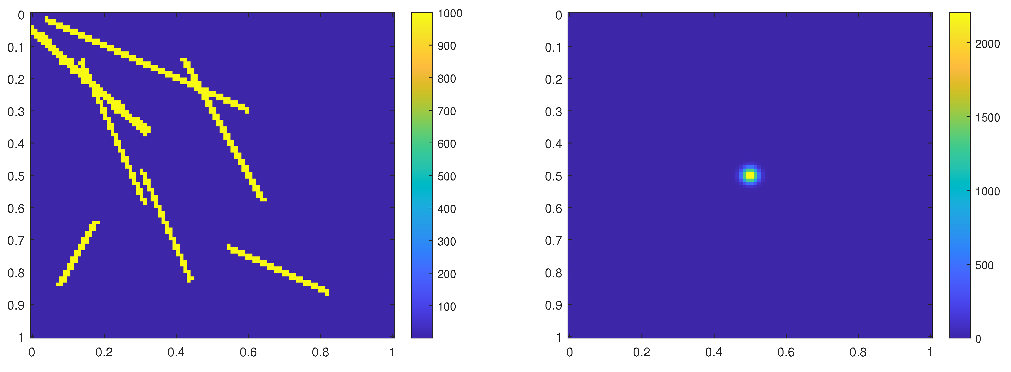
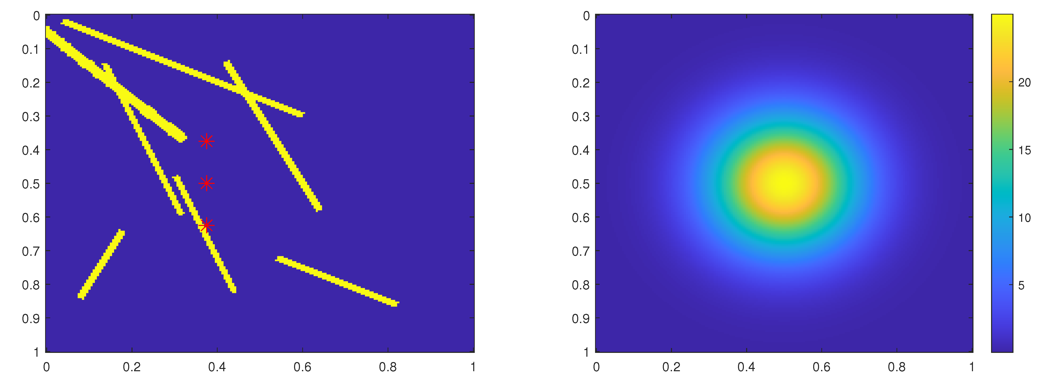
We consider the medium parameter depicted in Figure other (see Figure 1). Medium properties are high contrast and multiscale. We choose the source term as a source distrubuted in a small region as shown in Figure 1). It, f, is given by
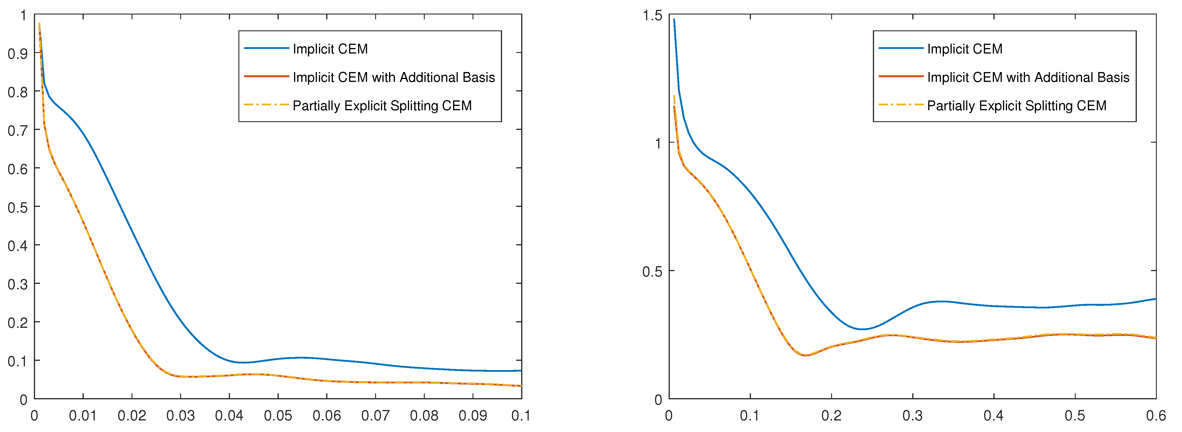
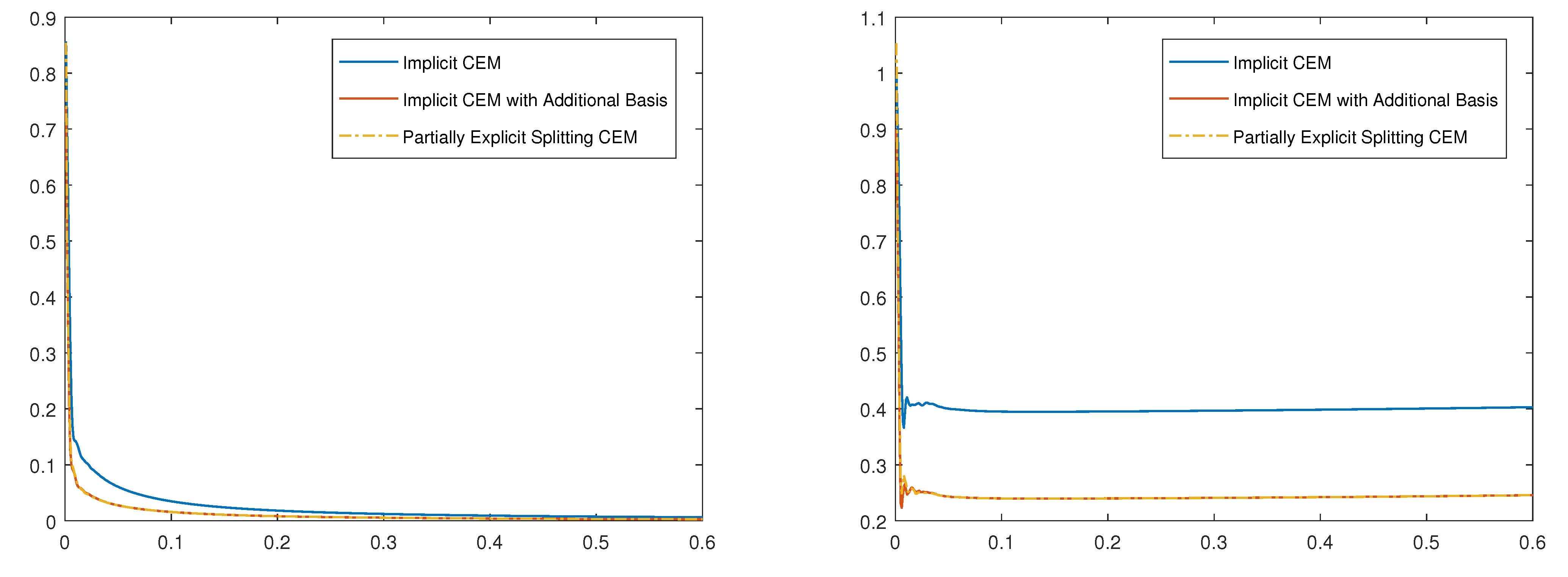
where is a frequency, which will be taken to be . We take the values for to be , , , and , which balances wave terms and parabolic terms. For larger ’s, we will observe slightly larger errors since the wave phenomena dominates. In all examples, we plot errors in time for three methods.
- Implicit CEM. In this, we use only implicit method with fewer degrees of freedom (without additional degrees of freedom) and compute the error associated with the multiscale approach.
- Implicit CEM with additional basis functions. In this approach, we take into account additional degrees of freedom and handle them in implicit manner. The method is more expensive and corresponds to full implicit approach.
- Partial Explicit Splitting CEM. In our approach, we take into account additional degrees of freedom and handle them in explicit manner. One approach for additional degrees is presented in Section 3.5.2. Partial Explicit Splitting CEM and Implicit CEM have the same degrees of freedom, while partial Explicit Splitting CEM handles additional degrees of freedom explicitly.
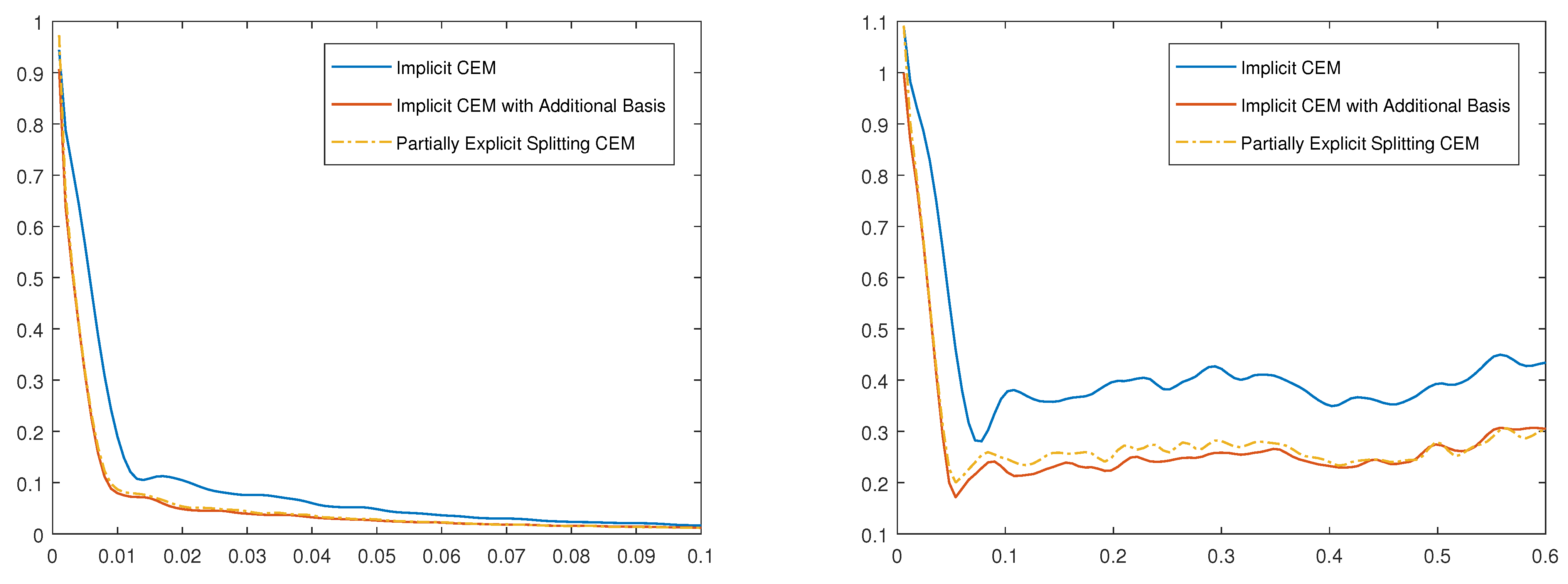
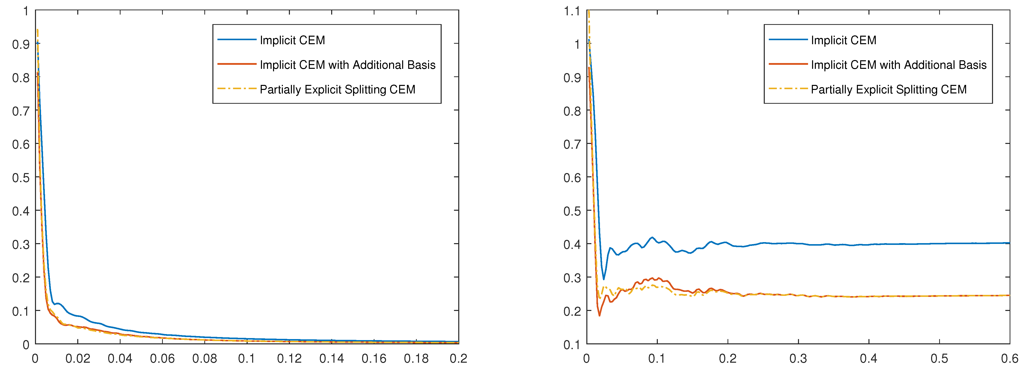
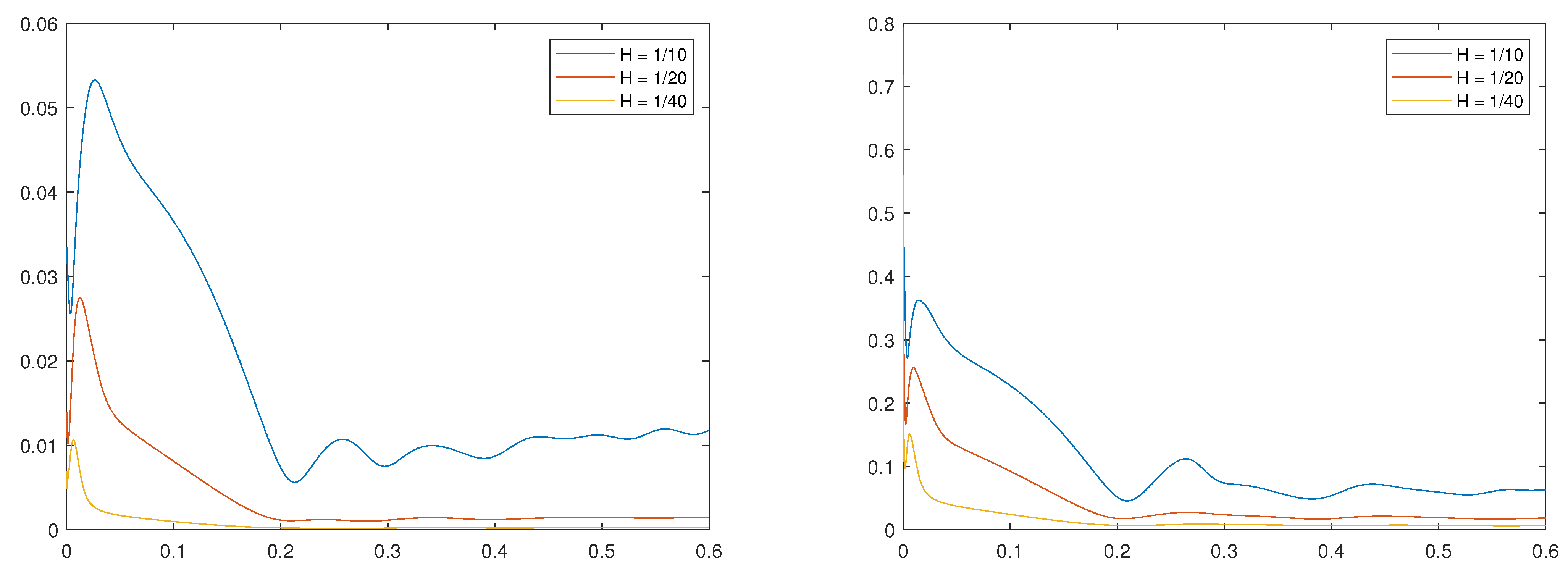
In Figure 2, we depict the results for the case and time step . As we see from the results that additional degrees of freedom improves the results. We note that in all examples, we choose the source term such that the error without additional degrees of freedom is large and we can improve it. In general, this error can be improved and made smaller with additional degrees of freedom. This is partially because of the source term which brings additional multiscale nature. Moreover, we observe that the errors of proposed partial explicit approach and fully implicit approach are similar. This suggest that our proposed approach is stable and can be used for explicit time stepping. In Figure 3, we use smaller , . In this case, we again observe similar phenomena, where our proposed approach provides very similar results when additional degrees of freedom treated implicitly. In other cases, we consider other values of , (see Figure 4) and (see Figure 5). In all cases, the proposed partial explicit approach provides very similar results compared to fully implicit approach when treating additional degrees of freedom. We note that because of nonzero right hand side, the energy can increase.
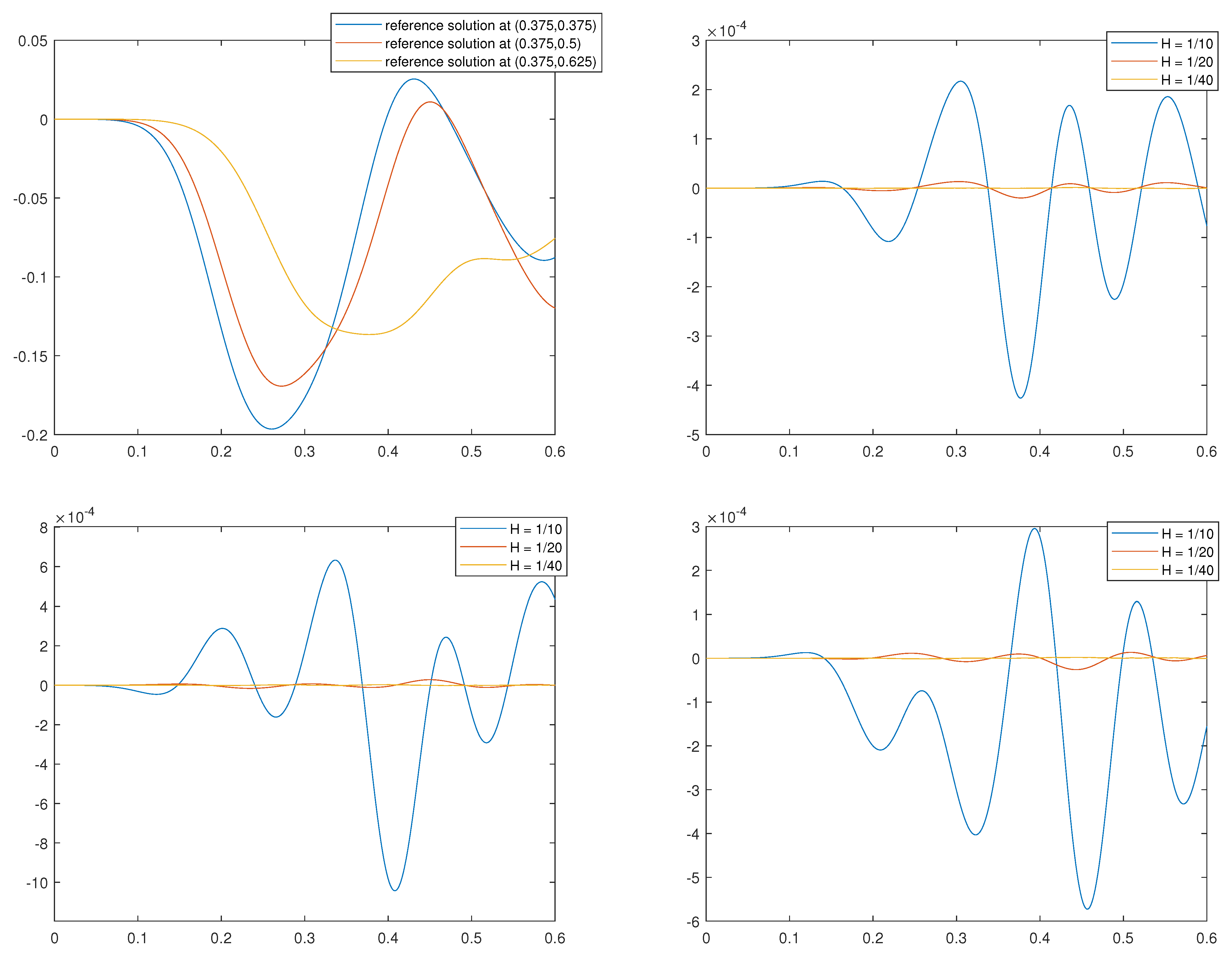
We will next present a numerical example with the same medium as the previous examples. We consider the source term is smoother spacially and with the same frequency as the previous example. In this case, we will have a much smaller error in both and Energy norm since the space can approximte the source better. In Figure 6, we show the medium with marker indicating three locations for comparison and the source term.
5. Conclusions
In this paper, we design and analyze contrast-independent partially explicit time discretization methods for quasi gas dynamics model. The proposed methods differ from our previous works [3,4] as parabolic and wave equations require different treatment for temporal and spatial discretization. Temporal splitting is based on spatial multiscale space splitting that we introduce in the paper. Using these multiscale spaces, time splitting identifies and treats fast components implicitly while slow component explicitly. Our proposed method is still implicit via mass matrix, which can be treated via mass lumping as in [4]. A stability of the proposed splitting is demonstrated under some conditions. The proposed method allows identifying the degrees of freedom that need explicit treatment and those that require implicit treatment. Numerical results show that the proposed methods provide very similar results as fully implicit methods using explicit methods with the time stepping that is independent of the contrast.
Author Contributions
Writing—review and editing, B.C., Y.E. and W.T.L. All authors have read and agreed to the published version of the manuscript.
Funding
This research received no external funding.
Institutional Review Board Statement
Not applicable.
Informed Consent Statement
Not applicable.
Data Availability Statement
Not applicable.
Acknowledgments
Y.E. would like to thank the partial support from NSF 1934904. Y.E. would also like to acknowledge the support of Mega-grant of the Russian Federation Government (N 14.Y26.31.0013).
Conflicts of Interest
The authors declare no conflict of interest.
References
- Chetverushkin, B.N.; D’Ascenzo, N.; Saveliev, A.V.; Saveliev, V. Kinetic model and magnetogasdynamics equations. Comput. Math. Math. Phys. 2018, 58, 691–699. [Google Scholar] [CrossRef]
- Chetverushkin, B.; Chung, E.; Efendiev, Y.; Pun, S.M.; Zhang, Z. Computational multiscale methods for quasi-gas dynamic equations. arXiv 2020, arXiv:2009.00068. [Google Scholar] [CrossRef]
- Chung, E.; Efendiev, Y.; Leung, W.T.; Vabishchevich, P.N. Contrast-independent partially explicit time discretizations for multiscale flow problems. arXiv 2021, arXiv:2101.04863. [Google Scholar] [CrossRef]
- Chung, E.; Efendiev, Y.; Leung, W.T.; Vabishchevich, P.N. Contrast-independent partially explicit time discretizations for multiscale wave problems. arXiv 2021, arXiv:2102.13198. [Google Scholar]
- Chung, E.; Efendiev, Y.; Leung, W.T. Constraint energy minimizing generalized multiscale finite element method. Comput. Methods Appl. Mech. Eng. 2018, 339, 298–319. [Google Scholar] [CrossRef] [Green Version]
- Chung, E.T.; Efendiev, Y.; Leung, W.T. Constraint energy minimizing generalized multiscale finite element method in the mixed formulation. Comput. Geosci. 2018, 22, 677–693. [Google Scholar] [CrossRef] [Green Version]
- Durlofsky, L. Numerical calculation of equivalent grid block permeability tensors for heterogeneous porous media. Water Resour. Res. 1991, 27, 699–708. [Google Scholar] [CrossRef] [Green Version]
- Allaire, G.; Brizzi, R. A multiscale finite element method for numerical homogenization. SIAM J. Multiscale Model. Simul. 2005, 4, 790–812. [Google Scholar] [CrossRef] [Green Version]
- Efendiev, Y.; Hou, T. Multiscale Finite Element Methods: Theory and Applications; Surveys and Tutorials in the Applied Mathematical Sciences; Springer: New York, NY, USA, 2009; Volume 4. [Google Scholar]
- Hou, T.; Wu, X. A multiscale finite element method for elliptic problems in composite materials and porous media. J. Comput. Phys. 1997, 134, 169–189. [Google Scholar] [CrossRef] [Green Version]
- Jenny, P.; Lee, S.; Tchelepi, H. Multi-scale finite volume method for elliptic problems in subsurface flow simulation. J. Comput. Phys. 2003, 187, 47–67. [Google Scholar] [CrossRef]
- Chung, E.T.; Efendiev, Y.; Hou, T. Adaptive multiscale model reduction with generalized multiscale finite element methods. J. Comput. Phys. 2016, 320, 69–95. [Google Scholar] [CrossRef] [Green Version]
- Chung, E.T.; Efendiev, Y.; Leung, W.T. Generalized multiscale finite element methods for wave propagation in heterogeneous media. Multiscale Model. Simul. 2014, 12, 1691–1721. [Google Scholar] [CrossRef] [Green Version]
- Chung, E.T.; Efendiev, Y.; Leung, W.T. Fast online generalized multiscale finite element method using constraint energy minimization. J. Comput. Phys. 2018, 355, 450–463. [Google Scholar] [CrossRef] [Green Version]
- Efendiev, Y.; Galvis, J.; Hou, T. Generalized multiscale finite element methods (GMsFEM). J. Comput. Phys. 2013, 251, 116–135. [Google Scholar] [CrossRef] [Green Version]
- Chung, E.T.; Efendiev, Y.; Leung, W.T.; Vasilyeva, M.; Wang, Y. Non-local multi-continua upscaling for flows in heterogeneous fractured media. J. Comput. Phys. 2018, 372, 22–34. [Google Scholar] [CrossRef] [Green Version]
- Owhadi, H.; Zhang, L. Metric-based upscaling. Commun. Pure. Appl. Math. 2007, 60, 675–723. [Google Scholar] [CrossRef]
- Weinan, E.; Engquist, B. Heterogeneous multiscale methods. Commun. Math. Sci. 2003, 1, 87–132. [Google Scholar]
- Henning, P.; Målqvist, A.; Peterseim, D. A localized orthogonal decomposition method for semi-linear elliptic problems. ESAIM Math. Model. Numer. Anal. 2014, 48, 1331–1349. [Google Scholar] [CrossRef] [Green Version]
- Roberts, A.; Kevrekidis, I. General tooth boundary conditions for equation free modeling. SIAM J. Sci. Comput. 2007, 29, 1495–1510. [Google Scholar] [CrossRef]
- Samaey, G.; Kevrekidis, I.; Roose, D. Patch dynamics with buffers for homogenization problems. J. Comput. Phys. 2006, 213, 264–287. [Google Scholar] [CrossRef] [Green Version]
- Marchuk, G.I. Splitting and alternating direction methods. Handb. Numer. Anal. 1990, 1, 197–462. [Google Scholar]
- Vabishchevich, P.N. Additive Operator-Difference Schemes: Splitting Schemes; Walter de Gruyter GmbH: Berlin, Germany; Boston, MA, USA, 2013. [Google Scholar]
- Ascher, U.M.; Ruuth, S.J.; Spiteri, R.J. Implicit-explicit Runge-Kutta methods for time-dependent partial differential equations. Appl. Numer. Math. 1997, 25, 151–167. [Google Scholar] [CrossRef]
- Li, T.; Abdulle, A. Effectiveness of implicit methods for stiff stochastic differential equations. Commun. Comput. Phys. 2008, 3, 295–307. [Google Scholar]
- Abdulle, A. Explicit methods for stiff stochastic differential equations. In Numerical Analysis of Multiscale Computations; Springer: Berlin/Heidelberg, Germany, 2012; pp. 1–22. [Google Scholar]
- Engquist, B.; Tsai, Y.H. Heterogeneous multiscale methods for stiff ordinary differential equations. Math. Comput. 2005, 74, 1707–1742. [Google Scholar] [CrossRef]
- Ariel, G.; Engquist, B.; Tsai, R. A multiscale method for highly oscillatory ordinary differential equations with resonance. Math. Comput. 2009, 78, 929–956. [Google Scholar] [CrossRef]
- Narayanamurthi, M.; Tranquilli, P.; Sandu, A.; Tokman, M. EPIRK-W and EPIRK-K time discretization methods. J. Sci. Comput. 2019, 78, 167–201. [Google Scholar] [CrossRef] [Green Version]
- Shi, H.; Li, Y. Local discontinuous Galerkin methods with implicit-explicit multistep time-marching for solving the nonlinear Cahn-Hilliard equation. J. Comput. Phys. 2019, 394, 719–731. [Google Scholar] [CrossRef]
- Duchemin, L.; Eggers, J. The explicit–implicit–null method: Removing the numerical instability of PDEs. J. Comput. Phys. 2014, 263, 37–52. [Google Scholar] [CrossRef] [Green Version]
- Frank, J.; Hundsdorfer, W.; Verwer, J. On the stability of implicit-explicit linear multistep methods. Appl. Numer. Math. 1997, 25, 193–205. [Google Scholar] [CrossRef] [Green Version]
- Izzo, G.; Jackiewicz, Z. Highly stable implicit–explicit Runge–Kutta methods. Appl. Numer. Math. 2017, 113, 71–92. [Google Scholar] [CrossRef]
- Ruuth, S.J. Implicit-explicit methods for reaction-diffusion problems in pattern formation. J. Math. Biol. 1995, 34, 148–176. [Google Scholar] [CrossRef]
- Hundsdorfer, W.; Ruuth, S.J. IMEX extensions of linear multistep methods with general monotonicity and boundedness properties. J. Comput. Phys. 2007, 225, 2016–2042. [Google Scholar] [CrossRef] [Green Version]
- Du, J.; Yang, Y. Third-order conservative sign-preserving and steady-state-preserving time integrations and applications in stiff multispecies and multireaction detonations. J. Comput. Phys. 2019, 395, 489–510. [Google Scholar] [CrossRef]
Figure 1.
Left: Medium ; Right: Source function f.

Figure 2.
. Left: error. Right: Energy error.

Figure 3.
. Left: error. Right: Energy error.

Figure 4.
. Left: error. Right: Energy error.

Figure 5.
. Left: error. Right: Energy error.

Figure 6.
Left: medium with marker indicating three locations for comparison, Right: source function f.
Figure 6.
Left: medium with marker indicating three locations for comparison, Right: source function f.

Figure 7.
. Left: error. Right: Energy error.

Figure 8.
Top-Left: Reference solution at different location. Top-Right: Error of the Partially Explicit scheme at location Bottom-Left: Error of the Partially Explicit scheme at location Bottom-Right: Error of the Partially Explicit scheme at location .
Figure 8.
Top-Left: Reference solution at different location. Top-Right: Error of the Partially Explicit scheme at location Bottom-Left: Error of the Partially Explicit scheme at location Bottom-Right: Error of the Partially Explicit scheme at location .

Publisher’s Note: MDPI stays neutral with regard to jurisdictional claims in published maps and institutional affiliations. |
© 2022 by the authors. Licensee MDPI, Basel, Switzerland. This article is an open access article distributed under the terms and conditions of the Creative Commons Attribution (CC BY) license (https://creativecommons.org/licenses/by/4.0/).
Share and Cite
MDPI and ACS Style
Chetverushkin, B.; Efendiev, Y.; Leung, W.T. Contrast-Independent Partially Explicit Time Discretizations for Quasi Gas Dynamics. Mathematics 2022, 10, 576. https://doi.org/10.3390/math10040576
AMA Style
Chetverushkin B, Efendiev Y, Leung WT. Contrast-Independent Partially Explicit Time Discretizations for Quasi Gas Dynamics. Mathematics. 2022; 10(4):576. https://doi.org/10.3390/math10040576
Chicago/Turabian StyleChetverushkin, Boris, Yalchin Efendiev, and Wing Tat Leung. 2022. "Contrast-Independent Partially Explicit Time Discretizations for Quasi Gas Dynamics" Mathematics 10, no. 4: 576. https://doi.org/10.3390/math10040576
Note that from the first issue of 2016, this journal uses article numbers instead of page numbers. See further details here.