Kinematic Model and Redundant Space Analysis of 4-DOF Redundant Robot

Abstract

The kinematics and redundant space analysis of redundant robots constitutes important research content. Currently, methods such as geometric method and iterative optimization method are relatively complicated and inconvenient for programming and practical control applications. Moreover, little research has been conducted on redundant space analysis. This paper takes the 4-DOF PowerCube redundant robot as the research object. The forward and inverse kinematics equation of the robot are established based on the D-H matrix method, projection and cosine theorem method, and vector coordinate method. Then, the redundant space of the robot is obtained and the redundant space range of the robot is analyzed. Finally, the simulation of kinematic and redundant space research is conducted. It is shown that the change of each joint angle of the robot is smooth without mutation, so it can ensure the stable motion of the robot. Additionally, the different position and redundant variable have a big influence on robotic configuration. The calculation amount is relatively small and convenient for programming application, and the path calculation data of the joints are obtained, which are conducive to the motion control of modular robots. The method used in this paper can be extended to the multi-DOF redundant robot. Finally, the motion optimization, control, and obstacle-avoidance of redundant robots are briefly studied. The results of this paper provide an important basis for these aspects of research.

1. Introduction

Compared with traditional robots, redundant robots have the advantages of good flexibility, good fault tolerance, and good coordination ability [1,2,3]. Singularity avoidance, obstacle avoidance, and performance optimization can be realized in redundant space. Therefore, redundant robot is being increasingly used in industry, coal mines, medical treatment, aerospace, and other fields and has become a hot research topic in the field of robots. In the kinematic analysis of redundant robots, especially in the inverse solution, due to the redundancy, the inverse kinematics solution is also complex. A kinematics solution and redundant space analysis are the basis for the research of redundant robots and provide a theoretical basis for obstacle avoidance planning [4,5,6], performance optimization, fault tolerance analysis, and motion control [7,8,9,10,11,12]. Therefore, it is of great significance to solve the kinematic model and analyze the redundant space of redundant robots. However, due to the existence of redundancy, the inverse solution and workspace analysis are more difficult and complicated.

At present, many experts and scholars have carried out extensive research in this field. K. Kreutez-Delgado et al. [13] gave the definition and determination of the arm angle for the first time and proposed to use the arm angle to describe the self-motion of the seven-degree of freedom (DOF) humanoid manipulator. However, a closed inverse kinematics solution related to arm angle redundant parameters is not derived. Instead, the velocity method based on the augmented Jacobian matrix is used to give the relationship between the joint angular velocity and the end velocity, as well as the arm angular velocity. Shimizu M [2] modified the original definition of the arm angle and redefined its reference plane to overcome the defect that the reference plane could not be determined when the vector and line coincided in the original definition, and deduced a closed inverse kinematics solution of the humanoid manipulator. At the same time, the influence of joint limit on the range of arm angle was analyzed. However, this method is more complicated and difficult to implement, and there may be some problems such as motion discontinuity. In 2013, Ding Xilun proposed using motion primitives to describe the motion of the humanoid manipulator, gave the inverse kinematics formula about motion primitives, and obtained the unique redundant solution. However, this method does not consider the effects of joint limit and collision [14]. Zhao Jianwen et al. used the subspace and motion manifold method to simulate the self-motion of the mechanism, solved the self-motion manifold at a given point, and verified it with the positive solution. This method has certain reference significance for solving the self-motion manifold of the spatially redundant robot, but this method is based on the geometric arm of the robot, which is more complex [15]. Xia Jing studied the kinematics solution and collision avoidance of the astronaut arm and proposed an analytical inverse kinematics solution of a redundant manipulator based on an arm angle [16]. Shi Jianping et al. [17] directly started from the forward kinematics equation of the manipulator. By reasonably constructing the optimization objective function, a method for solving the inverse kinematics of the manipulator based on the improved PSO algorithm is proposed. Xu Peng et al. [18] studied the multi-objective optimization problem of the inverse kinematics solution manifold of redundant robot. Combined with the proposed optimization objective function, the corresponding optimized inverse solution of the redundant robot was obtained. Based on the weighted minimum norm method, Yang Fangping [19] derived an optimization to avoid calculating the pseudo-inverse of the Jacobian matrix. Zhao Zhanfang [20] and Wang Yong et al. [21] studied the kinematics optimization problem in the gradient algorithm, but they mainly considered the selection of the motion amplification coefficient in their research. The calculation method is very complicated and thus is not conducive to real-time solution. Zu Di et al. [22] proposed a secondary calculation method to solve the inverse kinematics closed solution of the redundant manipulator. This method can ensure the accuracy and correct the error of the gradient projection method, but it increases the difficulty and complexity of the solution.

Additionally, Kouabon A et al. [23] parameterized a group of joints of redundant robots. Then, the inverse solution problem was transformed into the inverse kinematics problem of non-redundant robots. Yugui Yang [24] used the neural network method to obtain the motion data of the 7-DOF robot, and then the least square method and genetic algorithm were used to search for the optimal solution of the inverse solution. In Dong Hui and Swagat Kumar’s study [25,26], the neural network method was also used to solve the inverse kinematics of redundant robots. In the paper [27,28], according to the redundancy characteristics of the robot, the constraint function method was adopted to solve its kinematics through optimization. In order to solve the motion planning of a robot in an unknown environment, in Park S O et al.’s study [29], the Jacobian matrix and artificial potential field method were used to solve the kinematics.

In addition, experts such as Burdick, J.W. and Philippe Wenger also conducted in-depth research on redundant robots. In Burdick, J.W.’s paper [30], based on the recursive theory of screw method, the singular position of a 3R manipulator was obtained and the geometric explanation was given. This research provides a theoretical basis for the study of the posture change of robots while avoiding a singular position. Philippe Wenger studied the spatial topological mechanism of a 3R manipulator and concluded that the manipulator has similar kinematic characteristics in different topological domains and operation types [30,31,32]. Philippe Wenger also classified the manipulator and analyzed the poor kinematic performance. The research results are of great significance in the design of manipulators [33]. Moreover, Philippe Wenger also studied the motion planning of a parallel redundant robot, analyzed the posture of the robot under different working modes, and studied how to avoid singular configuration [34,35]. These studies played an important role in the field of redundant robots.

In summary, aiming at the kinematics and redundant space analysis of redundant robots, currently, most studies mainly focus on the plane-arm angle analysis method, constraint limitation method, iterative optimization method, neural network method, weighted minimum norm method, and pseudo-inverse method. These methods have an important reference significance for the related research of redundant robots. However, these methods have some disadvantages such as a large amount of calculation, the long learning time of the neural network, being very difficult to solve, and local minima and singular points [36,37]. As for the iterative optimization method [38,39,40,41], high accuracy can be achieved only when a very small step length is taken, but the convergence time will be very slow. Additionally, if the step size is too large, it will oscillate near the target coordinates. It is difficult to meet the real-time requirements in actual motion control using the abovementioned method. The kinematics model is the basis of robot research. In addition, a redundant robot, due to its redundancy characteristics, has a variety of configurations that do not affect its end pose. However, little research has been conducted on redundant space analysis.

In this paper, the SCHUNK PowerCube modular robot is taken as the research object. By locking part of the joints, it is equivalent to a 4-DOF redundant robot. Then, the kinematic model and redundant space analysis research are carried out. Firstly, the forward kinematics equation of the robot is obtained based on the D-H matrix method and the vector coordinate method. Then, the inverse kinematics model is obtained by using the projection method and cosine theorem method. Next, the redundant space of the robot is conducted based on the kinematics model. Finally, the redundant space range of the robot is analyzed. The method used in this paper can be extended to the multi-DOF redundant robot. Finally, the motion optimization, control, and obstacle avoidance of redundant robot are briefly studied. This research provides a theoretical basis for further study on redundant robots.

2. Kinematics Model

2.1. Robot Model

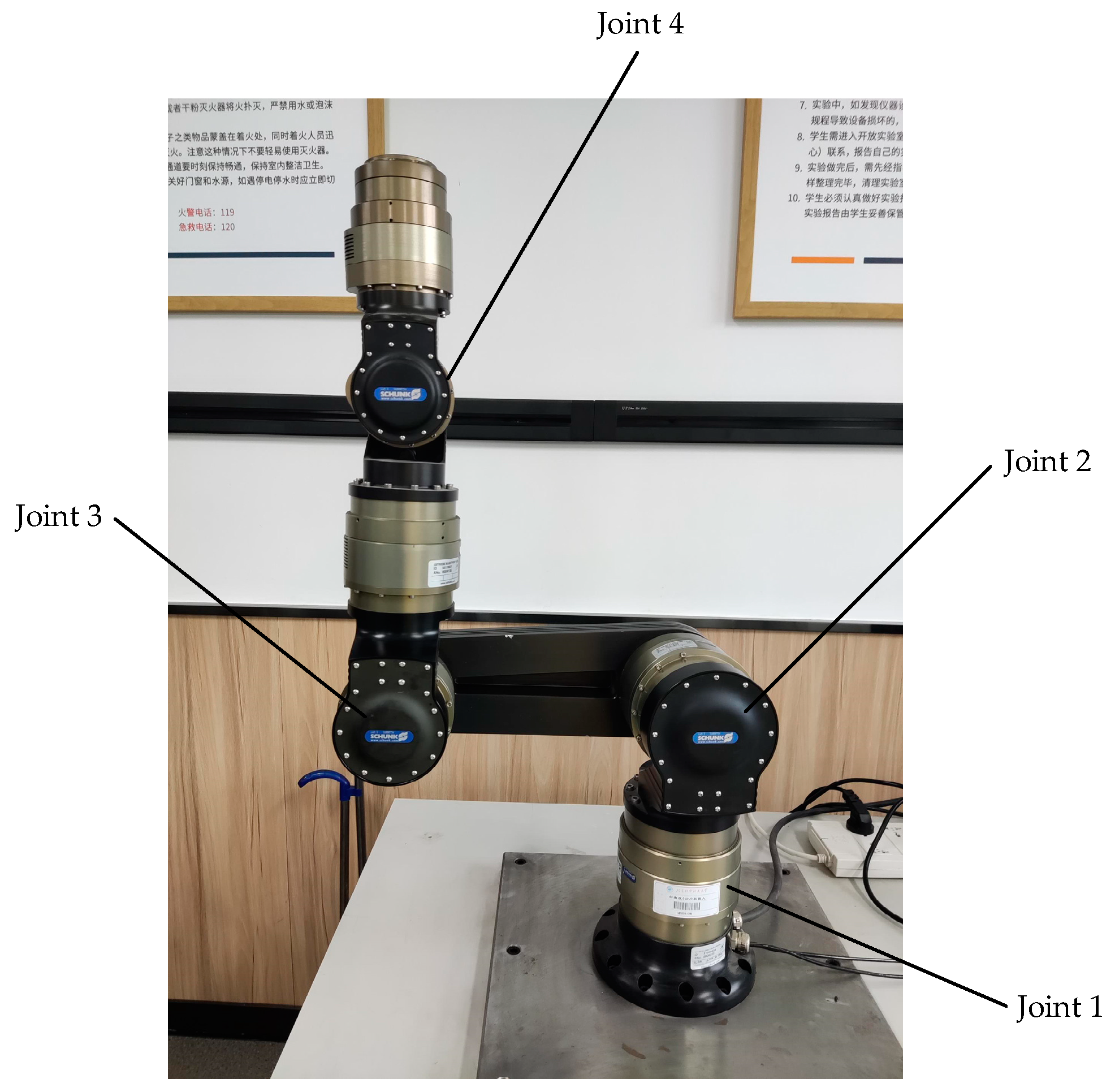
The BAUSATZLWA3 6 DOF+FWK050 SCHUNK robot in the laboratory is taken as the research object to conduct relevant research. It is a modular robot with 6-DOF. Due to the analysis of redundant robot, the 4th and 6th joints are locked and regarded as connecting rods. The axes of joint 2, joint 3, and joint 5 are parallel to each other. Then, the three joints can be regarded as a planar three-link mechanism. The base of the robot is a joint that rotates around the vertical direction. When it rotates, the robot can move in three-dimensional space. At this time, the robot becomes a 4-DOF robot. Because the number of joints is greater than the motion dimension, it is a redundant robot, and the redundancy is located on the three-link plane mechanism above the base. The structure of the robot is shown in Figure 1.

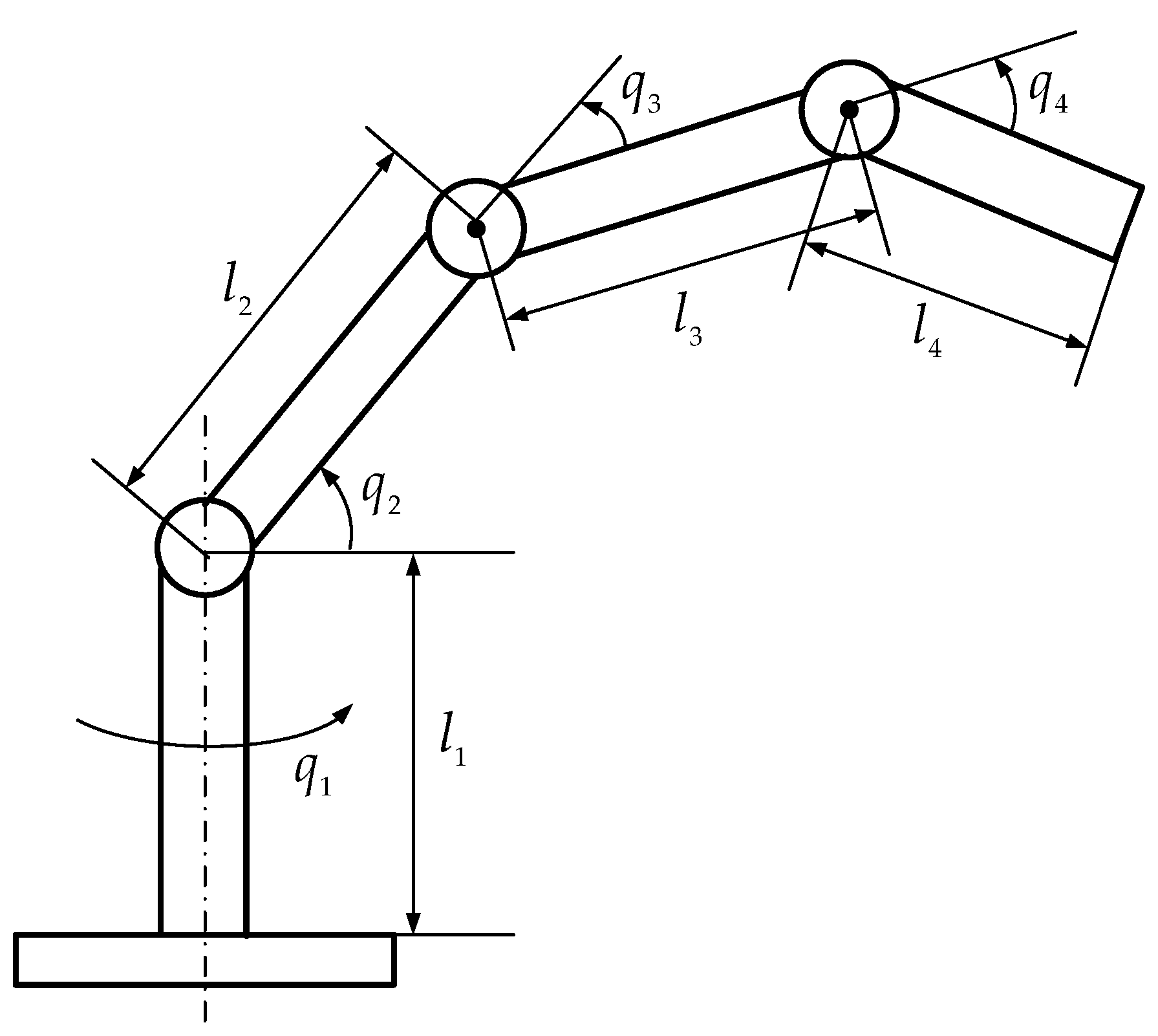
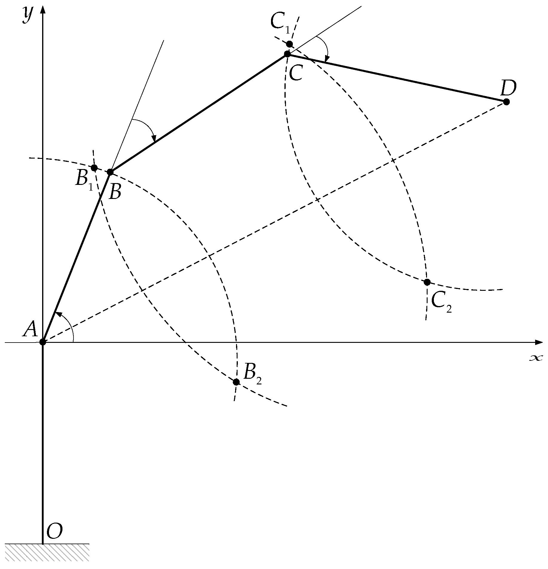
According to the structure model of the robot, its diagram is shown in Figure 2.

2.2. Forward Kinematics Model

The D-H homogeneous matrix transformation method is used to solve the kinematics equation of the robot. According to the robot structure, the D-H parameter can be obtained, as shown in

Table 1. D-H parameter.

$\mathit{i}$	${\mathit{a}}_{\mathit{i}-1}$	${\mathit{\alpha }}_{\mathit{i}-1}$ (°)	${\mathit{d}}_{\mathit{i}}$	${\mathit{q}}_{\mathit{i}}$
1	0	0	$l_1$	$q_1$
2	0	90	0	$q_2$
3	$l_2$	0	0	$q_3$
4	$l_3$	0	0	$q_4$
5	$l_4$	0	0	0

Note: Since the planar three-link mechanism carries out a coordinate transformation relative to the base, i.e., joint 1, so five groups of DH matrix transformation parameters are finally obtained.

.

The transformation matrix of the coordinate system after moving and rotating is

$${\mathrm{Rot}}_x({\alpha }_{i-1})=\left[\begin{array}{cccc}1& 0& 0& 0\\ 0& \cos {\alpha }_{i-1}& -\sin {\alpha }_{i-1}& 0\\ 0& \sin {\alpha }_{i-1}& \cos {\alpha }_{i-1}& 0\\ 0& 0& 0& 1\end{array}\right]$$

(1)

$${\mathrm{Trans}}_x(a_{i-1})=\left[\begin{array}{cccc}1& 0& 0& a_{i-1}\\ 0& 1& 0& 0\\ 0& 0& 1& 0\\ 0& 0& 0& 1\end{array}\right]$$

(2)

$${\mathrm{Rot}}_z(q_i)=\left[\begin{array}{cccc}\cos q_i& -\sin q_i& 0& 0\\ \sin q_i& \cos q_i& 0& 0\\ 0& 0& 1& 0\\ 0& 0& 0& 1\end{array}\right]$$

(3)

$${\mathrm{Trans}}_z(d_i)=\left[\begin{array}{cccc}1& 0& 0& 0\\ 0& 1& 0& 0\\ 0& 0& 1& d_i\\ 0& 0& 0& 1\end{array}\right]$$

(4)

The transformation matrix between the $i-1$-th and $i$-th coordinate systems is

$$\begin{array}{ll}{}_i{}^{i-1}T& ={\mathrm{Rot}}_x({\alpha }_{i-1}){\mathrm{Trans}}_x(a_{i-1}){\mathrm{Rot}}_z(q_i){\mathrm{Trans}}_z(d_i)\\ & =\left[\begin{array}{cccc}\cos q_i& -\sin q_i& 0& a_{i-1}\\ \sin q_i\cos {\alpha }_{i-1}& \cos q_i\cos {\alpha }_{i-1}& -\sin {\alpha }_{i-1}& -d_i\sin {\alpha }_{i-1}\\ \sin q_i\sin {\alpha }_{i-1}& \cos q_i\sin {\alpha }_{i-1}& \cos {\alpha }_{i-1}& -d_i\cos {\alpha }_{i-1}\\ 0& 0& 0& 1\end{array}\right]\end{array}$$

(5)

According to the homogeneous transformation rule, the transformation relations between coordinates are, respectively,

$${}_1{}^{0}T=\left[\begin{array}{cccc}\cos q_1& -\sin q_1& 0& 0\\ \sin q_1& \cos q_1& 0& 0\\ 0& 0& 1& l_1\\ 0& 0& 0& 1\end{array}\right]$$

(6)

$${}_2{}^{1}T=\left[\begin{array}{cccc}\cos q_2& -\sin q_2& 0& 0\\ 0& 0& -1& 0\\ \sin q_2& \cos q_2& 0& 0\\ 0& 0& 0& 1\end{array}\right]$$

(7)

$${}_3{}^{2}T=\left[\begin{array}{cccc}\cos q_3& -\sin q_3& 0& l_2\\ \sin q_3& \cos q_3& 0& 0\\ 0& 0& 1& 0\\ 0& 0& 0& 1\end{array}\right]$$

(8)

$${}_4{}^{3}T=\left[\begin{array}{cccc}\cos q_4& -\sin q_4& 0& l_3\\ \sin q_4& \cos q_4& 0& 0\\ 0& 0& 1& 0\\ 0& 0& 0& 1\end{array}\right]$$

(9)

$${}_5{}^{4}T=\left[\begin{array}{cccc}1& 0& 0& l_4\\ 0& 1& 0& 0\\ 0& 0& 1& 0\\ 0& 0& 0& 1\end{array}\right]$$

(10)

Then, the homogeneous transformation matrix between the end effector and the base is

$$\begin{array}{ll}{}_5{}^{0}T& ={}_1{}^{0}T{}_2{}^{1}T{}_3{}^{2}T{}_4{}^{3}T{}_5{}^{4}T\\ & =\left[\begin{array}{cccc}{c}_1{c}_{234}& -c_1{s}_{234}& s_1& (l_4{c}_{234}+l_3{c}_{23}+l_2{c}_2)c_1\\ s_1{c}_{234}& -s_1{s}_{234}& -c_1& (l_4{c}_{234}+l_3{c}_{23}+l_2{c}_2)s_1\\ s_{234}& c_{234}& 0& l_4{s}_{234}+l_3{s}_{23}+l_2{s}_2+l_1\\ 0& 0& 0& 1\end{array}\right]\end{array}$$

(11)

where $s_1=\sin q_1$, $c_1=\cos q_1$, $s_{12}=\sin (q_1+q_2)$, $c_{12}=\cos (q_1+q_2)$, $s_{123}=\sin (q_1+q_2+q_3)$, and $c_{123}=\cos (q_1+q_2+q_3)$.

Therefore, the position equation of the robot is

$$\{\begin{array}{l}x=[l_2\cos q_2+l_3\cos (q_2+q_3)+l_4\cos (q_2+q_3+q_4)]\cos q_1\hfill \\ y=[l_2\cos q_2+l_3\cos (q_2+q_3)+l_4\cos (q_2+q_3+q_4)]\sin q_1\hfill \\ z=l_1+l_2\sin q_2+l_3\sin (q_2+q_3)+l_4\sin (q_2+q_3+q_4)\hfill \end{array}$$

(12)

As for other alternative methods for directly obtaining the kinematics of the robot, we can also use the vector coordinate method. The detailed calculation process is as follows.

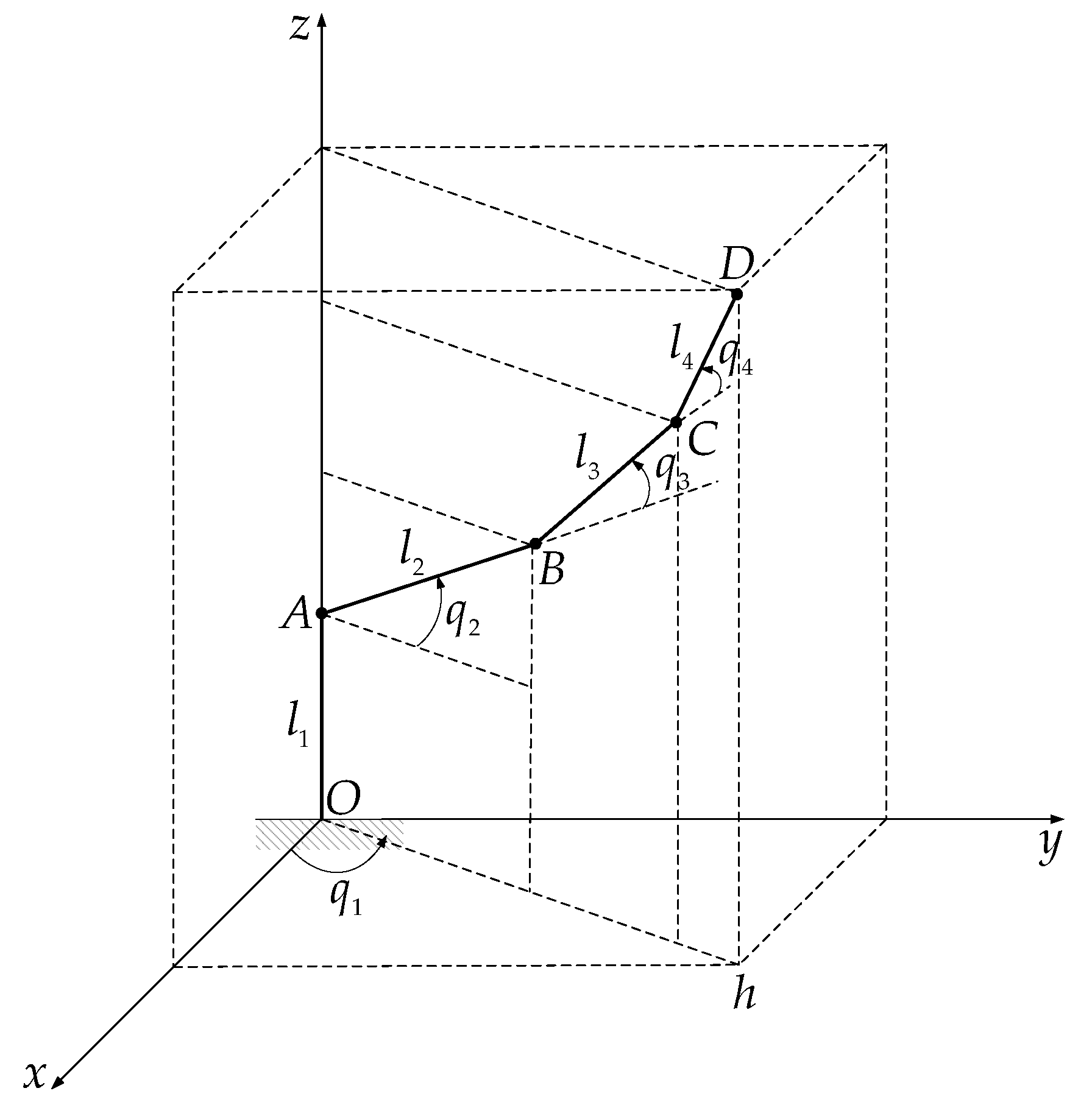
The coordinate diagram of the robot is shown in Figure 3.

If the base and rotation of the base $OA$ are not considered, $AB$, $BC$,$CD$ forms a planar three-link mechanism. On $hOz$ plane, setting the coordinate of end-effector $D$ as $(m,n)$, the following can be obtained:

$$\{\begin{array}{c}m=l_2\cos q_2+l_3\cos (q_2+q_3)+l_4\cos (q_2+q_3+q_4)\\ n=l_2\sin q_2+l_3\sin (q_2+q_3)+l_4\sin (q_2+q_3+q_4)\end{array}$$

(13)

When the base rotates, the motion range of the robot is the three-dimensional space, and the motion equation of the end can be obtained by projecting and decomposing the coordinate $(m,n)$, so in the $O\text{–}xyz$ space, the motion equation of the end-effector is

$$\{\begin{array}{l}x=m\cos q_1\hfill \\ y=m\sin q_1\hfill \\ z=l_1+n\hfill \end{array}$$

(14)

Thus,

$$\{\begin{array}{l}x=[l_2\cos q_2+l_3\cos (q_2+q_3)+l_4\cos (q_2+q_3+q_4)]\cos q_1\hfill \\ y=[l_2\cos q_2+l_3\cos (q_2+q_3)+l_4\cos (q_2+q_3+q_4)]\sin q_1\hfill \\ z=l_1+l_2\sin q_2+l_3\sin (q_2+q_3)+l_4\sin (q_2+q_3+q_4)\hfill \end{array}$$

(15)

Obviously, the result obtained by this method is the same as that obtained by D-H matrix transformation method.

Then, the speed is

$$\{\begin{array}{ll}\dot{x}& =[l_2\sin q_2+l_3\sin (q_2+q_3)](-\sin q_1){\dot{q}}_1\\ & +\cos q_1[l_2\cos q_2{\dot{q}}_2+l_3\cos (q_2+q_3)({\dot{q}}_2+{\dot{q}}_3)]\\ \dot{y}& =[l_2\sin q_2+l_3\sin (q_2+q_3)]\cos q_1{\dot{q}}_1\\ & +\sin q_1[l_2\cos q_2{\dot{q}}_2+l_3\cos (q_2+q_3)({\dot{q}}_2+{\dot{q}}_3)]\\ \dot{z}& =-l_2\sin q_2{\dot{q}}_2-l_3\cos (q_2+q_3)({\dot{q}}_2+{\dot{q}}_3)\end{array}$$

(16)

Jacobian matrix plays an important role in robot research, which reflects the transfer relationship between input and output of robot.

According to the definition of the Jacobian matrix, it can be obtained that

$$J(q)=\frac{\partial f(q)}{\partial q}$$

(17)

where

$$f(q)=\left[\begin{array}{c}x\\ y\\ z\end{array}\right]$$

(18)

Since the robot can move in three-dimensional space and there are four joints, the Jacobian matrix is a $3\times 4$ rectangular matrix. When analyzing the relationship between the Cartesian space and the joint space, Jacobian matrix is a rectangle matrix. Because it is a redundant robot, the number of equations is less than the number of unknowns. Then, the corresponding homogeneous equations are composed of general solutions and special solutions, in which all the non-zero solutions of the equations constitute the null space of Jacobian matrix. The above equations constitute forward kinematics model of the robot.

2.3. Inverse Kinematics Model

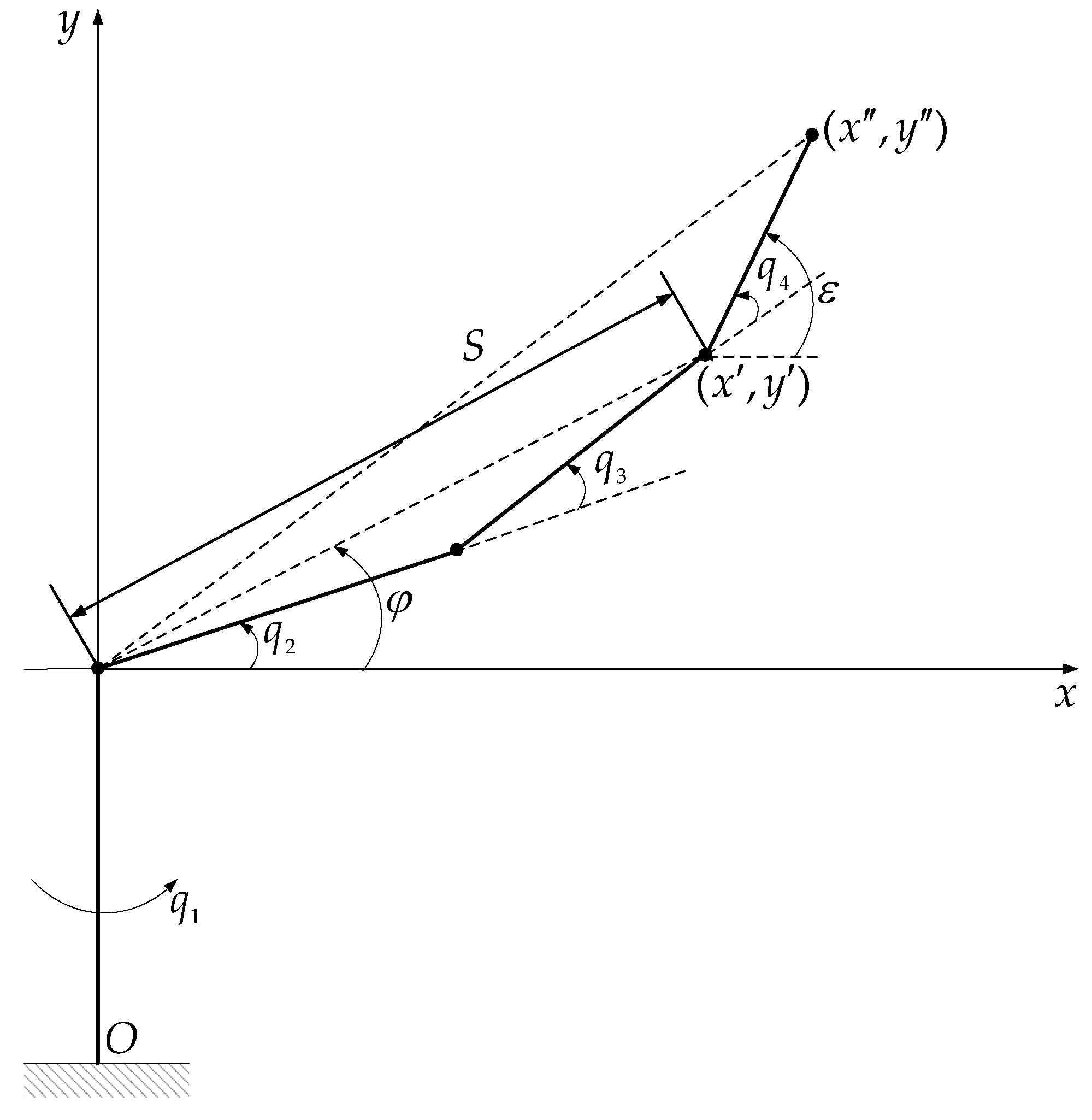
When solving the inverse solution of the robot, the inverse kinematics of the three-link mechanism above the base is calculated first. The position of the end of the two-link mechanism is set to $(x^{\prime },y^{\prime })$ by making auxiliary lines along the horizontal and vertical directions at the end points. The distance between the end point and the origin is $S=\sqrt{{x^{\prime }}^2+{y^{\prime }}^2}$. Taking $S$ as the hypotenuse, a right triangle is formed. The coordinate diagram of the mechanism is shown in Figure 4.

The angle passing through the origin is denoted as φ; then, there is

$$\phi =\arctan (\frac{y^{\prime }}{x^{\prime }})$$

(19)

$$x^{\prime }=S\cos \phi$$

(20)

$$y^{\prime }=S\sin \phi$$

(21)

Then

$$l_3\cos (q_2+q_3)=x^{\prime }-l_2\cos (q_2)$$

(22)

$$l_3\sin (q_2+q_3)=y^{\prime }-l_2\sin (q_2)$$

(23)

Equations (22) and (23) are squared, respectively, on both sides; then, by adding them together, we can get

$$l_3^2={x^{\prime }}^2+{y^{\prime }}^2+l_2^2-2l_2(x^{\prime }\cos (q_2)+y^{\prime }\sin (q_2))$$

(24)

Substituting Equations (20) and (21) into Equation (24), the following can be obtained:

$${x^{\prime }}^2+{y^{\prime }}^2+l_2^2-l_3^2=2S{l}_2(\cos (q_2)\cos (\phi )+\sin (q_2)\sin (\phi ))$$

(25)

That is,

$${x^{\prime }}^2+{y^{\prime }}^2+l_2^2-l_3^2=2S{l}_2\cos (q_2-\phi )$$

(26)

Additionally, ${x^{\prime }}^2+{y^{\prime }}^2=S^2$; combined with the cosine theorem, we get

$$\begin{array}{ll}{q}_2-\phi & =\pm \arccos \left(\frac{{x^{\prime }}^2+{y^{\prime }}^2+l_2^2-l_3^2}{2S{l}_2}\right)\\ & =\pm \arccos \left(\frac{S^2+l_2^2-l_3^2}{2S{l}_2}\right)\end{array}$$

(27)

So

$$q_2=\pm \arccos \left(\frac{{x^{\prime }}^2+{y^{\prime }}^2+l_2^2-l_3^2}{2S{l}_2}\right)+\phi$$

(28)

And

$${x^{\prime }}^2+{y^{\prime }}^2=l_2^2+l_3^2-2l_2{l}_3\cos (\pi -q_3)$$

(29)

Hence,

$$\pi -q_3=\arctan (\frac{l_2^2+l_3^2-{x^{\prime }}^2+{y^{\prime }}^2}{2l_2{l}_3})$$

(30)

$$q_3=\pi -\arccos (\frac{l_2^2+l_3^2-{x^{\prime }}^2+{y^{\prime }}^2}{2l_2{l}_3})$$

(31)

The end position of the three-link mechanism above the base is $(x^{″},y^{″})$. The angle between the third connecting link and the horizontal plane is denoted as ε; then,

$$\epsilon =\arctan (\frac{y^{″}}{x^{″}})$$

(32)

Since

$$\epsilon =q_2+q_3+q_4$$

(33)

So, the third joint angle of three-link mechanism is

$$q_4=\epsilon -q_2-q_3$$

(34)

When the base rotates $q_1$ angle, it forms a three-dimensional motion space. At this moment, the end position is recorded as $(x,y,z)$. The solution expression of rotation angle is as follows:

$$q_1=\arctan (\frac{y}{x})$$

(35)

In the three-dimensional space, the coordinate designation form used in the previous inverse solution of the planar three-link mechanism is changed. Projecting the coordinates of three-dimensional space to horizontal plane, there are

$$x^{″}=\sqrt{x^2+y^2} (\mathrm{or} x^{″}=\frac{x}{\cos q_1})$$

(36)

$$y^{″}=z-l_1$$

(37)

$$x^{\prime }=x^{″}-l_4\cos \epsilon$$

(38)

$$y^{\prime }=y^{″}-l_4\sin \epsilon$$

(39)

The above is the inverse kinematics model of 4-DOF redundant robot. The angle ε between the third connecting link and the horizontal plane is redundant variable. When ε changes, the other two joint angles of the connecting link also change, which reflects the redundancy characteristics of the mechanism. This provides a theoretical basis for the redundant space analysis.

For multi-joint and multi-redundant DOF robot, when solving its kinematics model, we can use the solution model and method of 4-DOF redundant robot to obtain the recursive equation of kinematics. Firstly, the position coordinates of the rotating mechanism on the same plane are obtained. If the base joint rotates, then the coordinates are decomposed and projected.

Here, we classify the robot joints as the same plane rotation joint and the rotation joint around the base. We divide the robot joint into the same plane rotation joint and the rotation joint around the base. The rotation joint in the same plane and the length of corresponding link are $q_1,q_2,\cdots q_i$, $l_1,l_2,\cdots l_i$, respectively. The rotation joint around the base and the length of corresponding link are ${\alpha }_1,{\alpha }_2,\cdots {\alpha }_k$, $r_1,r_2,\cdots r_k$, respectively.

Set the angle between each link and the horizontal plane as Φ_i thus,

$${\Phi }_i={\Phi }_{i-1}+q_i$$

(40)

So, the kinematic equation on the plane is

$$\{\begin{array}{l}{x}_i^p=x_{i-1}^p+l_i\cos {\Phi }_i\hfill \\ y_i^p=y_{i-1}^p+l_i\sin {\Phi }_i\hfill \end{array}$$

(41)

When the base rotates, the motion range of the robot is the three-dimensional space, and the motion equation of the end can be obtained by projecting and decomposing the coordinate $(x_i^p,y_i^p)$, so in the $O\text{–}xyz$ space, kinematic equation of the end-effector is

$$\{\begin{array}{l}{x}_i^s=x_i^p\cos {\alpha }_k\hfill \\ y_i^s=x_i^p\sin {\alpha }_k\hfill \\ z_i^s=r_k+y_i^p\hfill \end{array}$$

(42)

Similarly, when solving the inverse kinematics of the robot, the position of end-effector is projected in three directions, and then the variation expression of each joint angle is obtained through geometric relationship. When studying the multi-DOF redundant robot, according to the joint configuration of the robot, the kinematics model can be piecewise calculated from the position of end-effector to the front joint, which involves not only the planar mechanism but also the rotation joint. Therefore, the kinematics of multi-DOF and multi-redundant DOF robot can be solved in segments by using the research method in this paper.

3. Redundant Space Analysis

An important feature of redundant robot is its self-motion, which refers to multiple joints that move together without affecting the end motion state. The column on the base of this 4-DOF robot rotates around the vertical direction. The last three links, i.e., link 2, link 3, and link 4, are parallel to each other. These three links form a planar two-dimensional mechanism. When the first joint of the robot starts to rotate, the planar three-link mechanism will also rotate. Therefore, the robot can move in three-dimensional space, that is, the motion range of robot is a three-dimensional space. Because the number of joints is 4 and the motion dimension in Cartesian space is 3, the robot will have redundant range. Through analysis, the redundant range of the robot is generated on planar three-link mechanism. Link 3 is regarded as a redundant link, and its corresponding driving angle is regarded as a redundant angle. According to the link connection relationship, the redundant range of other links is obtained.

As shown in Figure 5, point $D$ is regarded as the end fixed point. To ensure that the position of point $D$ remains unchanged, the following conditions must be met.

As for the left point of link 3, first of all, this point is also the right point of link 2. Therefore, this point is located on the circle with the radius of the length of link 2. At the same time, as the left point of link 3, its motion range cannot exceed the range of the circle with the radius of the sum of the radii of link 2 and link 3. Therefore, the left point of the link 3 should be located on the arc corresponding to the intersection of the above two circles. As for the right point of link 3, first of all, this point is also the left point of link 4. Therefore, this point is located on the circle with the radius of the length of link 4. At the same time, as the right point of link 3, its motion range cannot exceed the range of the circle with the radius of the sum of the radii of link 3 and link 4. Therefore, the right point of the link 3 should be located on the arc corresponding to the intersection of the above two circles. That is, $B$ is on the arc $B_1{B}_2$ and $C$ is on the arc $C_1{C}_2$. Finally, the length between the left point and the right point, i.e., $BC$, should be the length of link 3.

When the above conditions are met, the obtained link configuration will constitute the redundant space of the robot, as shown in Figure 5.

4. Numerical Simulation

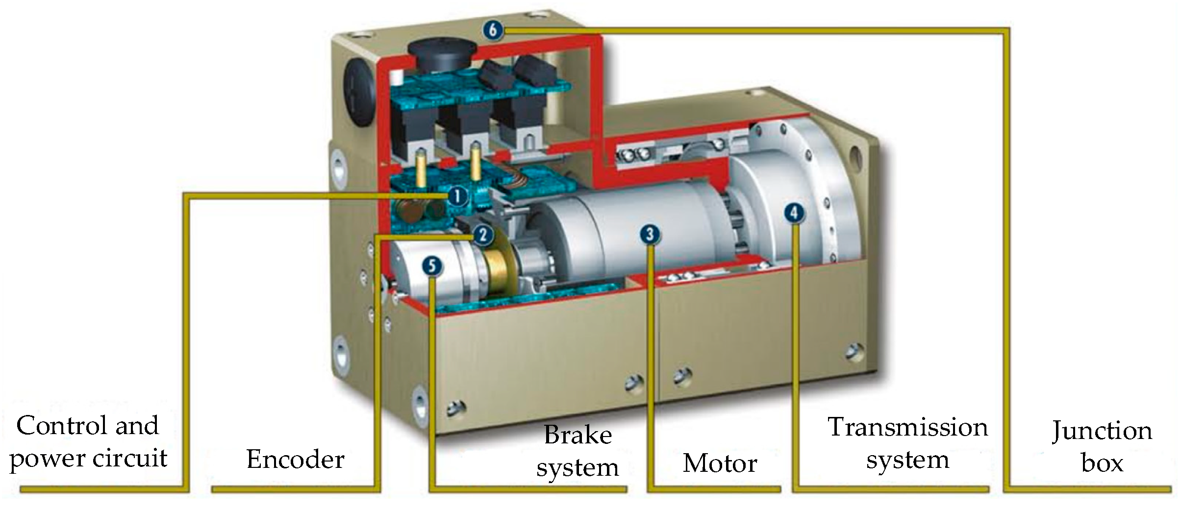
The SCHUNK PowerCube robot in the laboratory integrates motion control, power system, and transmission system. The module adopts a general communication interface without setting up a separate control cabinet. The integrated system is shown in Figure 6.

The robot is based on PowerCube control software for data exchange and can bus for communication. According to the robot product data and actual measurement, the structural parameters of the robot are shown in

Table 2. Structural parameters of the robot.

Structural Parameters	Numerical Value
$l_1$ (cm)	30
$l_2$ (cm)	30
$l_3$ (cm)	30
$l_4$ (cm)	20

Note: $l_i(i=1,2,3,4)$ refers to the length of link $i$.

.

After giving the motion trajectory of the end effector, the change of joint angle is obtained according to the inverse kinematics model. Motion trajectories are as follows, and the exercise time is 3 s.

$$\{\begin{array}{l}x=10\sin (\frac{2\pi }{3}t)\\ y=5\sin (\frac{2\pi }{3}t)+10\\ z=-10\cos (\frac{2\pi }{3}t)+40\end{array}$$

(43)

$$\{\begin{array}{l}x=10\sin (\frac{2\pi }{3}t)\\ y=5\sin (\frac{2\pi }{3}t)+10\\ z=30-20t\end{array}$$

(44)

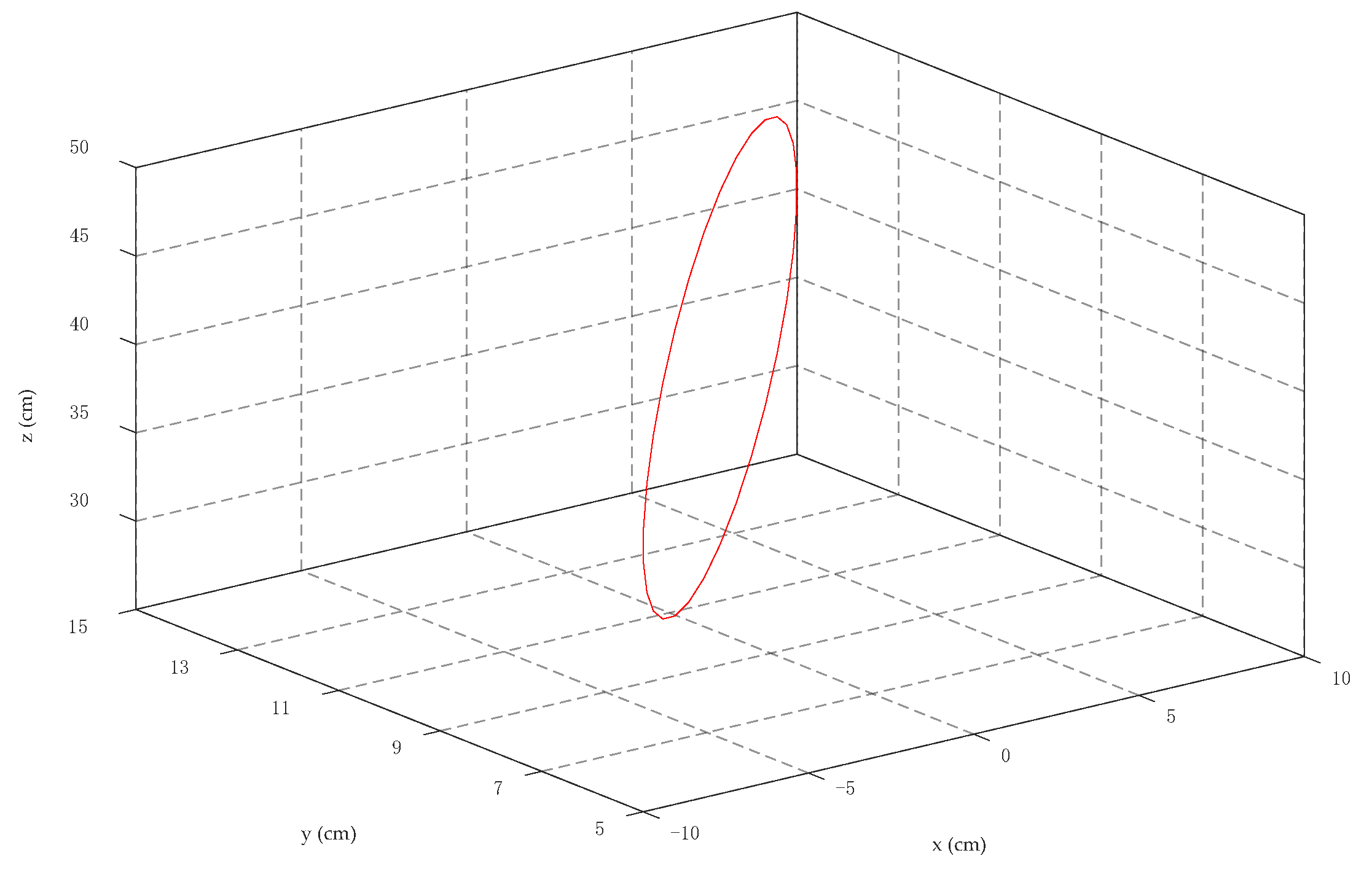
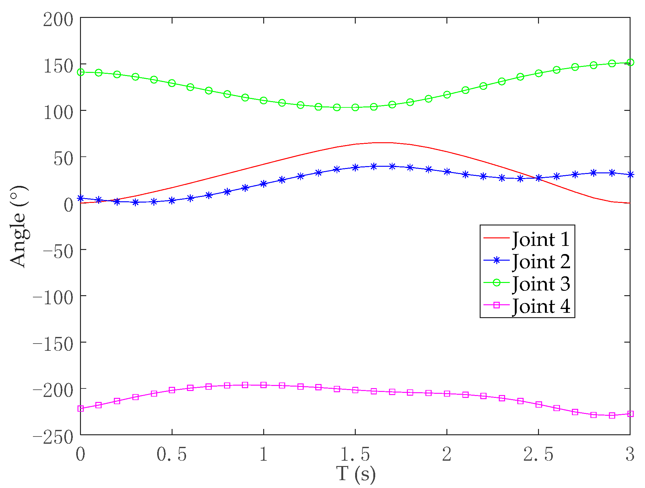
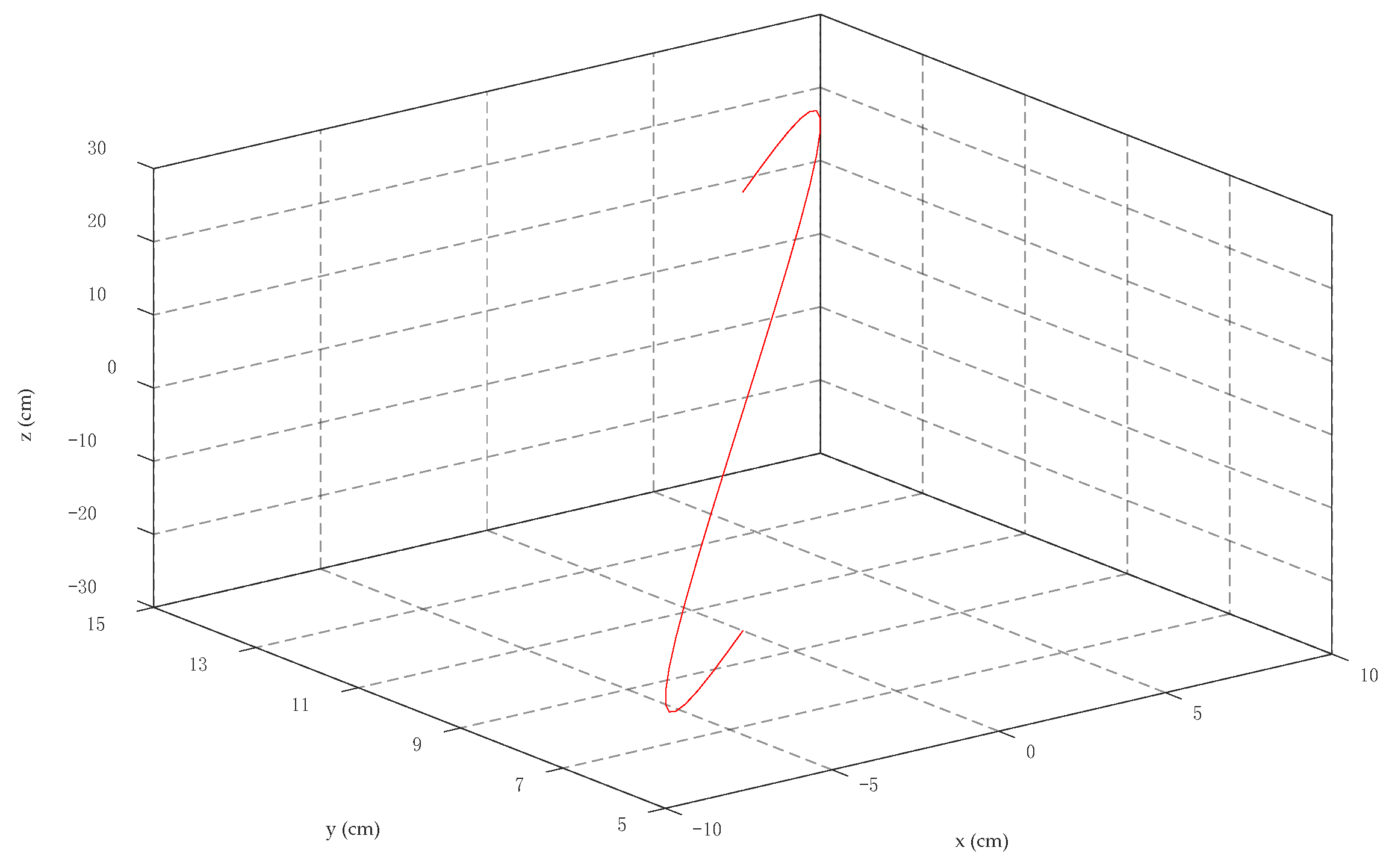
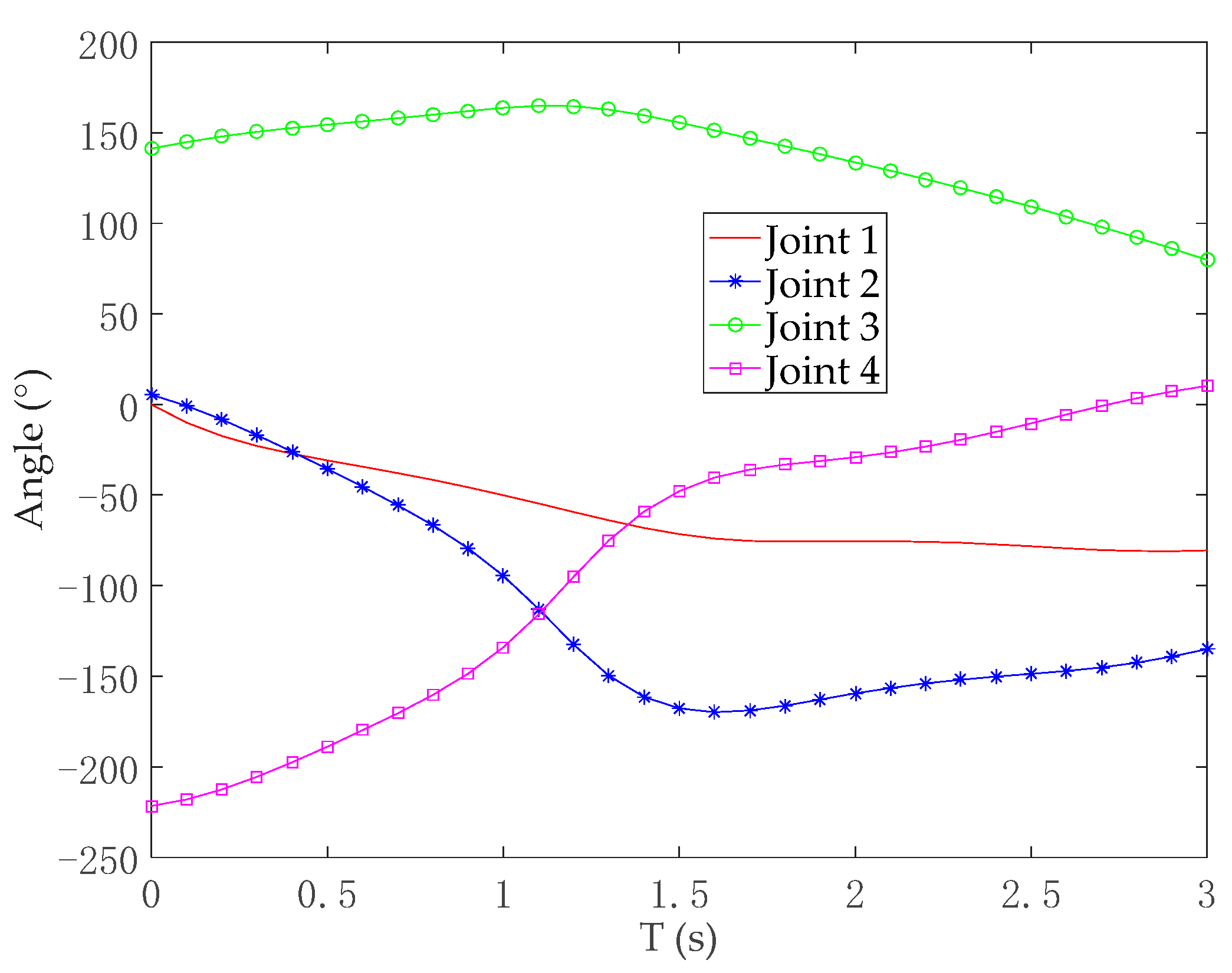
When the motion equation is Equation (43), the motion trajectory in space and the change curves of four joint angles are shown in Figure 7 and Figure 8, respectively.

When the motion equation is Equation (44), the motion trajectory in space and the change curves of four joint angles are shown in Figure 9 and Figure 10, respectively.

Based on the established model, the angle changes of each joint of the robot are obtained, which lays an important foundation for trajectory planning and motion control of the robot. Among them, the angle $\epsilon$ is randomly obtained as a redundant variable. In future research, it could be used to realize the obstacle avoidance while completing the tracking task. The simulation shows that the change of each joint angle of the robot is smooth without mutation. So, it can ensure the stable motion of the robot. The relationship between the solution equation of joint angle and the end trajectory equation is obvious. The calculation amount is relatively small and easy to program. The path calculation data of joints is obtained, which is conducive to motion control of the modular robot.

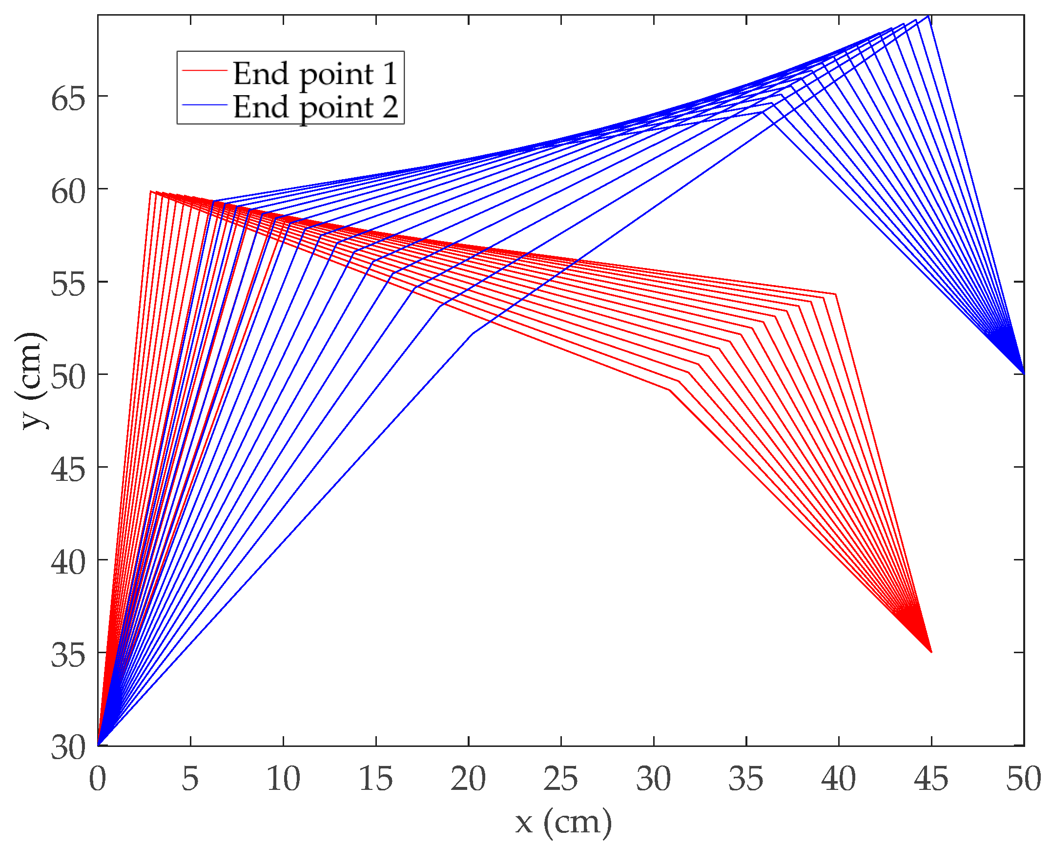
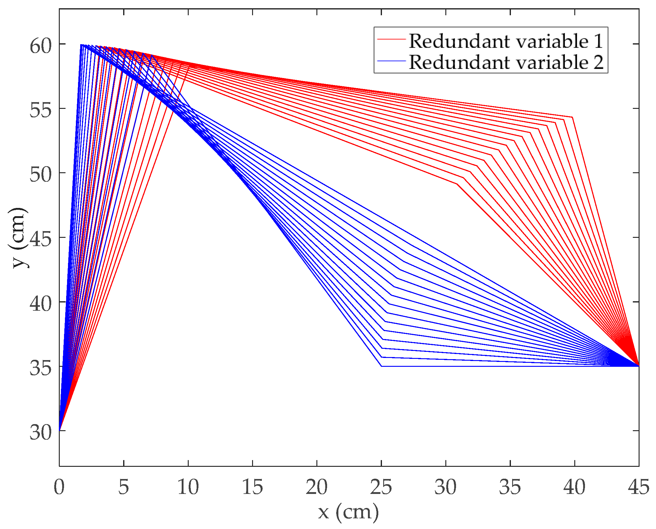
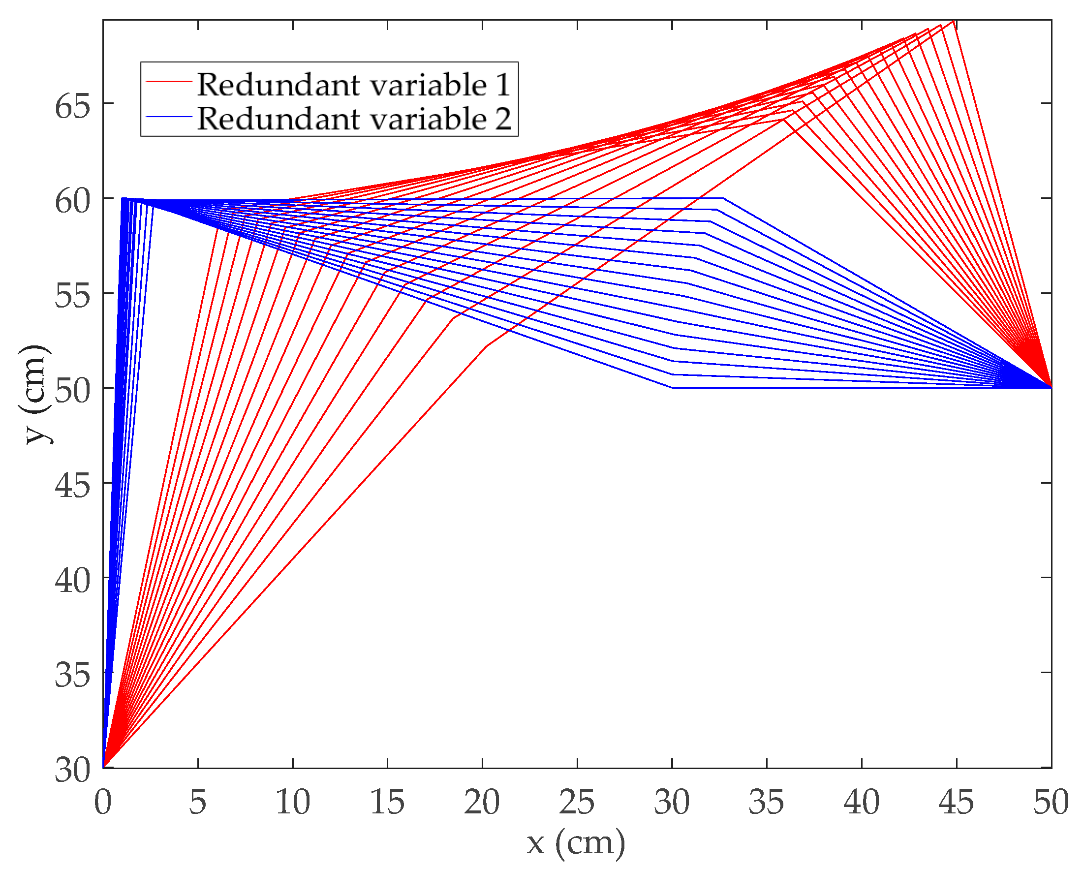
When the robot base, i.e., the first joint $q_1$, does not rotate, the entire robot becomes a planar mechanism, and its motion range is in the $x\text{-}y$ plane. Taking the base as the coordinate origin and the end points of the robot as $D_1(45,35)$ and $D_2(50,50)$ and setting the free motion range ${\epsilon }_1\in [-{75}^{°},-{45}^{°}]$, ${\epsilon }_2\in [-{75}^{°},-{60}^{°}]$, then the simulation is carried out respectively, as is shown in Figure 11, Figure 12 and Figure 13.

From the Figure 11, Figure 12 and Figure 13, the changes of redundant range under different points and different free motion ranges are obtained, respectively. The simulation results of redundant space show that when the end of the robot is at different positions, even if the interval length of the redundant range and the initial value and the final value of the redundant range are same, there is still a big difference in the configuration of the robot. Namely, the end position will have a greater impact on the range of variation of other joints. Moreover, when the end position is fixed, the interval length of the redundant range is the same, but for different initial values and the final values, the motion range of other joints is very different. Accordingly, the end position of the robot, the size of the redundancy range, and the initial and final value of the redundancy range have a great influence on the configuration of other joints.

This research provides an important theoretical reference for trajectory planning, obstacle avoidance in redundant space, task hierarchical control, and motion optimization control of redundant robot. The contents in this aspect are briefly introduced as follows.

The trajectory planning requires the robot to have good motion flexibility. When redundant robots perform a task, there are many configurations. Therefore, regarding trajectory planning, the performance optimization of redundant robots, such as manipulability, should be studied.

The manipulability is the evaluation index of robot flexibility, which is defined as

$$M=\sqrt{\det (J{J}^{\mathrm{T}})}$$

(45)

According to the knowledge of matrix theory, it can be obtained

$$M={\xi }_1{\xi }_2\cdots {\xi }_{\mathrm{n}}$$

(46)

where ${\xi }_1,{\xi }_2,\cdots {\xi }_{\mathrm{n}}$ refers to the eigenvalue of Jacobian matrix $J$.

When the robot approaches the singular configuration, the minimum eigenvalue of the Jacobian matrix is close to zero. At this moment, the manipulability $M\to 0$. In other words, the greater the manipulability of the robot, the more flexible it is.

The Jacobian matrix is related to the joint configuration of the robot. We hope that the robot can perform tasks in a better configuration, so the robot control is transformed into an optimization problem. It involves objective function and constraint conditions, and the specific mathematical model is as follows.

$$\{\begin{array}{l}\max M=\sqrt{\det (J{J}^{\mathrm{T}})}\hfill \\ s.t.\hfill \\ q_{\min }\le q\le q_{\max }\hfill \\ {\tau }_{\min }\le \tau \le {\tau }_{\max }\hfill \end{array}$$

(47)

where $q_{\min },{\tau }_{\min },q_{\max },{\tau }_{\max }$ correspond to lower bound and upper bound of $q,\tau$, respectively.

According to the optimization model, the optimal joint angle is obtained. Based on the joint data, the trajectory planning can be carried out. Then, the PD negative feedback method is used to realize the motion control of the robot.

For obstacle avoidance task, the redundant space of the robot is used to avoid the obstacle without affecting the terminal motion. Here, the concept of virtual repulsive force acting on the connecting link is introduced. The obstacle avoidance speed increases with the decrease of distance. By detecting the minimum distance between the obstacle and the robot, the corresponding redundant range of the robot, i.e., the joint variation range, can be obtained and recorded as $q\in [q_{\min }\begin{array}{c}\end{array}{q}_{\max }]$. Then, the redundant parameter $\epsilon$ can be determined. Finally, PD negative feedback is applied to the robot for motion control, and the obstacle avoidance in the null space can be conducted.

5. Conclusions

This paper takes the SCHUNK PowerCube modular robot in our laboratory as a research object. By locking part of joints, it is equivalent to a 4-DOF redundant robot. Then, the kinematic model and redundant space analysis research are carried out. Based on the established model, the simulation shows that the change of each joint angle of the robot is smooth and without mutation. So, it can ensure the stable motion of the robot. The relationship between the solution equation of joint angle and the end trajectory equation is obvious. The calculation amount is relatively small and easy to program. Additionally, the path calculation data of the joints are obtained, which is conducive to the motion control of the modular robot. The projection method and cosine theorem method in this paper are of great significance for analyzing the kinematics, especially the inverse solution model of a multi-DOF redundant robot.

Additionally, the simulation results of redundant space show that when the end effector of the robot is in different positions, even if the interval length of the redundant range and the initial value and the final value of the redundant range are same, there is still a big difference in the configuration of the robot. Namely, the end position will have a greater impact on the range of variation of other joints. Moreover, when the end position is fixed, the interval length of the redundant range is the same, but for a different initial value and the final value, the motion range of other joints is very different. Accordingly, the end position of the robot, the size of the redundancy range, and the initial and final value of the redundancy range have a great influence on the configuration of other joints. Based on the results, the motion optimization, control, and obstacle avoidance of a redundant robot are briefly studied. The research of this paper provides an important basis for these aspects of research.

In the future, I will further study how to select redundant parameters to avoid singularity.