Inverse Sum Indeg Index (Energy) with Applications to Anticancer Drugs

Abstract

For a simple graph with vertex set $\{v_1,v_2,\dots ,v_n\}$ with degree sequence $d_{v_i}$ of vertex $v_i,i=1,2,\dots ,n$, the inverse sum indeg matrix ($ISI$-matrix) $A_{ISI}\left(G\right)={\left(a_{ij}\right)}_{n\times n}$ of G is defined by $a_{ij}=\frac{d_{v_i}{d}_{v_j}}{d_{v_i}+d_{v_j}},$ if $v_i$ is adjacent to $v_j$, and zero, otherwise. The multiset of eigenvalues of $A_{ISI}\left(G\right)$ is the $ISI$-spectrum of G and the sum of their absolute values is the $ISI$-energy of $G$. In this paper, we modify the two results of (Li, Ye and Broersma, 2022), give the correct characterization of the extremal graphs and thereby obtain better bounds than the already known results. Moreover, we also discuss the QSPR analysis and carry the statistical modelling (linear, logarithmic and quadratic) of the physicochemical properties of anticancer drugs with the $ISI$-index (energy).

1. Introduction

Topological indices are the interesting attributes to analyse the physicochemical properties and the characteristics of chemical structures. There are certain important types of topological indices (degree, distance, spectral, and others including their mixed invariants). Here, we consider a degree-based topological index, the $ISI$-index, and its spectral invariant, the $ISI$-energy, on anticancer drug molecular structures. Basically, a topological index is generated by converting a molecular structure to a numeric value. Practically, the chemical compounds are taken as a graph where the elements are vertices and the bonds connecting them are edges. The anticancer drugs in this study are considered as chemical compounds, and their underlying graphs are considered. These topological indices and their spectral invariants are utilised in quantitative structure–property relationships (QSPR) studies to determine the bioactivity of chemical compounds. Cancer is a very deadly disease and is a rapid increase of abnormal/dead cells in the body. Carcinogens are the substances that are the cause of cancer. A carcinogen is a chemical substance with certain molecules such as tobacco smoke. It has the property of spreading to other parts of body. Some symptoms of this deadly disease include lumps, abnormal bleeding, prolonger cough, weight loss, anxiety, etc. Some causes of cancer are chewing tobacco, obesity, bad diet, laziness, large intakes of alcohol. Cancer can be cured by several treatments such as surgery, radiotherapy, chemotherapy, hormone therapy, targeted therapy and more. Anticancer drugs are drugs which are used to treat cancer, including alkylates and metabolites. Chemical graph theory is a discipline of mathematical chemistry that deals with the chemical graphs which represent chemical systems. Chemical graph theory defines topological indices on graphs and in particular the chemical structures of alkanes/anticancer drugs. In this work, several chemical graph structures of drugs (see Figure 1) are taken and a QSPR analysis is carried out on various anticancer drug structures to determine their physical characteristics and chemical reactions along with their $ISI$-index and $ISI$-energy (see definitions in the following paragraph). For a similar type of analysis, see [1,2,3,4,5,6].

Let $G=G(V,E)$ be a graph with vertex set $V=\{v_1,v_2,\dots ,v_n\}$ and edge set E. We consider only simple and undirected graphs, unless otherwise stated. The number of elements in V is the order n and the number of elements in E is the size m of G. By $u\sim v$, we mean a vertex u is adjacent to a vertex v. We denote an edge by $uv$ connecting two vertices u and v. The neighbourhood (open neighbourhood) $N\left(v\right)$ of $v\in V$ is the set of vertices adjacent to v. The degree $d_v$ of a vertex v is the number of elements in the set $N\left(v\right)$. A graph G is called r-regular, if $d_v=r$ for each v. We denote the complete graph by $K_n$, the complete bipartite graph by $K_{a,b}$ and the complete q partite graph by $K_{n_1,n_2,\dots ,n_q}$. We follow the standard graph theory notation, and more graph theoretic notations can be found in [7].

The adjacency matrix $A\left(G\right)$ of G is a square matrix of order n, with the $(i,j)$th entry equal to 1, if $v_i\sim v_j$, and $0,$ otherwise. Clearly, $A\left(G\right)$ is a real symmetric matrix and its multiset of eigenvalues is known as the spectrum of G. Let ${\lambda }_1\ge {\lambda }_2\ge \cdots \ge {\lambda }_n$ be the eigenvalues of $A\left(G\right)$, where the eigenvalue ${\lambda }_1$ is called the spectral radius of G. More about the adjacency matrix $A\left(G\right)$ can be seen in [7,8].

The energy [9] of G is defined by

$$\mathcal{E}\left(G\right)=\sum _{i=1}^n\left|{\lambda }_i\right|.$$

The energy is intensively studied in both mathematics and theoretical chemistry, since it is the trace norm of real symmetric matrices in linear algebra and the total $\pi$-electron energy of a molecule in mathematical chemistry, see [10,11]. For more information about the energy of G, including recent developments, see [12,13,14].

The inverse sum indeg index (shortly $ISI$-index) [15] is a topological index defined as

$$ISI\left(G\right)=\sum _{uv\in E\left(G\right)}\frac{d_u{d}_v}{d_u+d_v}.$$

The $ISI$-index is a well-studied topological index and it has many applications in quantitative structure–activity or structure–property relationships (QSAR/QSPR) [1,3,4,16].

The inverse sum indeg matrix ($ISI$-matrix) of a graph G, introduced by Zangi, Ghorbani and Eslampour [17], is a square matrix of order n, and it is defined by

$$A_{ISI}\left(G\right)={\left(a_{ij}\right)}_n=\left\{\begin{array}{cc}\frac{d_{v_i}{d}_{v_j}}{d_{v_i}+d_{v_j}}\hfill & \mathrm{if}{v}_i\sim v_j\hfill \\ 0\hfill & \mathrm{otherwise}.\hfill \end{array}\right.$$

The $ISI$-matrix is real and symmetric, and its eigenvalues can be indexed from the largest to the smallest as

$${\tau }_1\ge {\tau }_2\ge \cdots \ge {\tau }_n.$$

The multiset of all eigenvalues of $ISI$-matrix of G is known as the $ISI$-spectrum of G, and the largest eigenvalue ${\tau }_1$ is called the $ISI$-spectral radius of $G.$ If an eigenvalue $\tau$ of $ISI$-matrix occurs with algebraic multiplicity $k\ge 2$, then we represent it by ${\tau }^{\left[k\right]}$. The $ISI$-energy of G is defined by

$${\mathcal{E}}_{ISI}\left(G\right)=\sum _{i=1}^n\left|{\tau }_i\right|.$$

Zangi et al. [17] gave basic properties of the $ISI$-matrix including the bounds for the $ISI$-energy of graphs. Hafeez and Rashid [18] obtained the $ISI$-spectrum and $ISI$-energy of special graphs. They also gave some bounds on the $ISI$-energy of graphs. Bharali et al. [19] gave some bounds on the $ISI$-energy and introduced the $ISI$ Estrada index of G. Havare [1] obtained the $ISI$ index and $ISI$-energy of the molecular graphs of hyaluronic acid–paclitaxel conjugates. For other properties of the $ISI$-index, $ISI$-matrix, $ISI$ Laplacian (signless) matrix and other recent results, see [20,21,22].

In Section 2, we modify the two results of [21], characterize the correct extremal graphs and thereby obtain better results than the already known results. In Section 3, we carry a statistical analysis of various anticancer drugs, give their correlation coefficients with the $ISI$-index and the $ISI$-energy along with their applications in quantitative structure–property relationship. We end the article with a conclusion.

2. Inverse Sum Indeg Energy of Graphs

We start with some already known results, which are used in the sequel.

Lemma 1 

([23]). Let G be a connected graph of order $n\ge 2$. Then, G has exactly two distinct $ISI$-eigenvalues if and only if G is a complete graph.

Lemma 2 

([23]). Let G be a bipartite graph. Then, G has three distinct $ISI$-eigenvalues if and only if G is a complete bipartite graph.

The following observation states that G has a symmetric $ISI$-spectrum towards the origin if G is bipartite.

Remark 1. 

Clearly, the $ISI$-matrix of the bipartite graph G can be written as

$$ISI\left(G\right)=\left(\begin{array}{cc}\mathbf{0}& B\\ B^T& \mathbf{0}\end{array}\right).$$

If τ is an eigenvalue of $ISI\left(G\right)$ with associated eigenvector $X={(x_1,x_2)}^T$, then it is clear that $ISI\left(G\right)X=\tau X$. Moreover, it is easy to see that $ISI\left(G\right)X^{\prime }=-\tau X^{\prime },$ where $X^{\prime }={(x_1,-x_2)}^T.$ This implies that the $ISI$-eigenvalues of a bipartite graph are symmetric about the origin.

Let ${\sigma }_i,i=1,2,\dots ,n$ be the singular values of the $n\times n$ matrix M. The Frobenius norm of M is defined by

$${\parallel M\parallel }_F^2={\sigma }_1^2+{\sigma }_2^2+\cdots +{\sigma }_n^2.$$

The sum of the squares of the eigenvalues (Frobenius norm of a real symmetric matrix) of the $ISI$-matrix (Theorem 5, [17]) is

$$\parallel A_{ISI}{\left(G\right)\parallel }_F^2=\sum _{i=1}^n{\tau }_i^2=2\sum _{v_i{v}_j\in E\left(G\right)}{\left(\frac{d_{v_i}{d}_{v_j}}{d_{v_i}+d_{v_j}}\right)}^2=2R=Tr\left(A_{ISI}^2\left(G\right)\right),$$

(1)

where $R={\displaystyle \sum _{v_i{v}_j\in E\left(G\right)}}{\left(\frac{d_{v_i}{d}_{v_j}}{d_{v_i}+d_{v_j}}\right)}^2,$ and $Tr$ is the trace of the the matrix.

The invariant $R={\displaystyle \sum _{v_i{v}_j\in E\left(G\right)}}{\left(\frac{d_{v_i}{d}_{v_j}}{d_{v_i}+d_{v_j}}\right)}^2$ is an important parameter related to the $ISI$-matrix and is repeatedly used in our results. We establish sharp bounds for it.

Proposition 1. 

Let G be a connected graph of order $n\ge 2$ with maximum degree Δ and minimum degree $\delta$. Then, the following holds:

(i) 

$$\frac{m{\delta }^2}{4}\le R\le \frac{m{\mathsf{\Delta }}^2}{4},$$

with equality if and only if G is regular.

(ii) 

$$R\le \frac{n{\tau }_1^2}{2(n-1)},$$

with the equality holding if and only if $G\cong K_n.$

(iii) 

Let G be a bipartite graph with $p\ge 1$ positive $ISI$-eigenvalues. Then,

$$R\ge p{\tau }_1^2,$$

with the equality holding if and only if G is a complete bipartite graph.

Proof. 

By the definition of R and Lemma 2.2 [20], for any edge $uv\in E\left(G\right)$, $\frac{\delta }{2}\le \frac{d_u{d}_v}{d_u+d_v}\le \frac{\mathsf{\Delta }}{2},$ with the equality holding if and only if G is regular. Now, part (i) follows.

(ii). Applying the Cauchy–Schwarz inequality to the vector (${\tau }_2,{\tau }_3,\dots ,{\tau }_n$), we have

$${\tau }_1^2=2R-\sum _{i=2}^n{\tau }_i^2\le 2R-\frac{1}{n-1}{\left(\sum _{i=2}^n{\tau }_i\right)}^2=2R-{\displaystyle \frac{1}{n-1}}{\tau }_1^2,$$

(2)

with the equality holding in (2) if and only if ${\tau }_2={\tau }_3=\cdots ={\tau }_n.$

Thus, from the above, it follows that

$$R\le \frac{n{\tau }_1^2}{2(n-1)}.$$

(3)

Suppose the equality holds in (3). Then, the equality holds in (2), which is possible if and only if ${\tau }_2={\tau }_3=\cdots ={\tau }_n,$ that is, G has two distinct $ISI$-eigenvalues. By Lemma 1, G is a complete graph.

(iii). Using ${\tau }_1^2+{\tau }_2^2+\cdots +{\tau }_n^2=2R,$ the property that G has p positive $ISI$-eigenvalues and noting that G has a symmetric $ISI$-spectrum towards the origin (Remark 1), we have

$$2\left({\tau }_1^2+{\tau }_2^2+\cdots +{\tau }_p^2\right)=2R,$$

which implies that $R\ge p{\tau }_1^2$, with the equality holding if and only $p=1.$ By Lemma 2, G is a complete bipartite graph. □

The following two results on the $ISI$-energy of graphs in terms of the size m, the smallest degree $\delta$ and the smallest eigenvalue ${\tau }_n$ were given by Li, Ye and Broersma [21], (see Theorems 12 and 14).

Theorem 1 

([21], Theorem 12). Let G be a connected graph of order $n>1$ with m edges and minimum degree $\delta .$ Then,

$${\mathcal{E}}_{ISI}\ge \delta \sqrt{m},$$

and the equality holds if and only if $G\cong K_{\frac{n}{2},\frac{n}{2}}.$

Theorem 2 

([21], Theorem 14). Let G be a connected graph of order $n>1$ with m edges and minimum degree $\delta .$ Then,

$${\mathcal{E}}_{ISI}\ge \left|{\tau }_n\right|+\sqrt{m{\delta }^2-3{\tau }_n^2},$$

and the equality holds if and only if $G\cong K_{\frac{n}{2},\frac{n}{2}}.$

We restate Theorems 1 and 2 in terms of the invariant R and characterize the correct extremal graphs.

Theorem 3. 

Let G be a connected graph of order $n\ge 2$. Then,

$${\mathcal{E}}_{ISI}\ge 2\sqrt{R},$$

with the equality holding if and only if G is the complete bipartite graph.

Theorem 4. 

Let G be a connected graph of order $n\ge 2$ and ${\tau }_n$ be the smallest $ISI$-eigenvalue. Then,

$${\mathcal{E}}_{ISI}\ge \left|{\tau }_n\right|+\sqrt{4R-3{\tau }_n^2}.$$

The equality holds if and only if G is either a complete bipartite or a complete tripartite graph.

We illustrate the above four theorems with the help of the following examples.

Ex.1

For $G\cong K_{3,5}$, the $ISI$-spectrum of G is $\{7.26184,0^{\left[6\right]},-7.26184\}$ and ${\mathcal{E}}_{ISI}\left(G\right)=14.5237$. Theorem 1 gives ${\mathcal{E}}_{ISI}\left(G\right)\ge 3\sqrt{15}=11.619$, Theorem 2 gives ${\mathcal{E}}_{ISI}\left(G\right)\ge |-7.26184|+\sqrt{15{\left(3\right)}^2-3{(-7.26184)}^2}=7.26184+\sqrt{-23.20296}$, which is imaginary, while Theorem 3 gives ${\mathcal{E}}_{ISI}\left(G\right)=2\sqrt{{\left(7.26184\right)}^2}=14.5237$ and Theorem 4 gives ${\mathcal{E}}_{ISI}\left(G\right)=|-7.26184|+\sqrt{4{\left(7.26184\right)}^2-3{(-7.26184)}^2}=14.5237.$

Ex.2

For $G\cong K_{9,8}$, the $ISI$-spectrum of G is $\{35.93774,0^{\left[15\right]},-35.9377\}$ and ${\mathcal{E}}_{ISI}\left(G\right)=71.8753$. Theorem 1 gives

$${\mathcal{E}}_{ISI}\left(G\right)\ge 8\sqrt{72}=67.8823,$$

Theorem 2 gives ${\mathcal{E}}_{ISI}\left(G\right)\ge \left|35.93774\right|+\sqrt{72{\left(8\right)}^2-3{\left(35.93774\right)}^2}=63.0199$, Theorem 3 gives ${\mathcal{E}}_{ISI}\left(G\right)=2\sqrt{{\left(35.93774\right)}^2}=71.8753$ and Theorem 4 gives ${\mathcal{E}}_{ISI}\left(G\right)=|-35.937744|+\sqrt{4{\left(35.93774\right)}^2-3{(-35.937744)}^2}=71.87537.$

Ex.3

For $G\cong K_{4,4,4}$, the $ISI$-spectrum of G is $\{32,0^{\left[9\right]},{(-16)}^{\left[2\right]}\}$ and ${\mathcal{E}}_{ISI}\left(G\right)=64$. Theorem 1 gives ${\mathcal{E}}_{ISI}\left(G\right)\ge 8\sqrt{48}=55.4256$, Theorem 2 gives ${\mathcal{E}}_{ISI}\left(G\right)\ge |-32|+\sqrt{48{\left(8\right)}^2-3{(-16)}^2}=64$, while $R=768$ Theorem 3 gives ${\mathcal{E}}_{ISI}\left(G\right)=2\sqrt{768}=55.4256$ and Theorem 4 gives ${\mathcal{E}}_{ISI}\left(G\right)=|-16|+\sqrt{4\left(768\right)-3{(-16)}^2}=64.$

Ex.4

For $G\cong C{S}_{5,3}$, the $ISI$-spectrum of G is $\{20.2893,0^{\left[2\right]},{(-3.5)}^{\left[4\right]},-6.28925\}$ and ${\mathcal{E}}_{ISI}\left(G\right)=40.5785$. Theorem 1 gives ${\mathcal{E}}_{ISI}\left(G\right)\ge 5\sqrt{25}=25$, Theorem 2 gives ${\mathcal{E}}_{ISI}\left(G\right)\ge |-6.28925|+\sqrt{25{\left(5\right)}^2-3{(-6.28925)}^2}=28.791$, with $R=250.104$, Theorem 3 gives ${\mathcal{E}}_{ISI}\left(G\right)=2\sqrt{250.104}=31.6294$ and Theorem 4 gives

$${\mathcal{E}}_{ISI}\left(G\right)=|-6.28925|+\sqrt{4\left(31.6294\right)-3{(-6.28925)}^2}=35.9836.$$

Ex.5

The graph obtained from $K_{\omega }$ and the path $P_l$ by adding an edge between any vertex of $K_{\omega }$ and one end vertex of $P_l$ is denoted by $P{K}_{\omega ,l}$. It is known as a path complete graph or kite graph. The pineapple graph $P(\omega ,n-\omega )$ is a graph obtained from $K_{\omega }$ by attaching $n-\omega$ pendent vertices at any vertex of $K_{\omega }.$ For $G\cong P{K}_{3,9}$, the $ISI$-spectrum of G is

$$\begin{array}{cc}\hfill \{2.55192,1.87374,& 1.5389,1.07415,0.559209,0.069339,-0.413158,-0.939312,-1,\hfill \\ \hfill & -1.43693,-1.81746,-2.06039\},\hfill \end{array}$$

and ${\mathcal{E}}_{ISI}\left(G\right)=15.3345$. Theorem 1 gives ${\mathcal{E}}_{ISI}\left(G\right)\ge 1\sqrt{12}=3.4641$, Theorem 2 gives ${\mathcal{E}}_{ISI}\left(G\right)\ge |-2.06039|+\sqrt{12{\left(1\right)}^2-3{(-2.06039)}^2}=2.06039+\sqrt{-0.73562}$, which is imaginary. Moreover, $R=12.7645$, Theorem 3 gives ${\mathcal{E}}_{ISI}\left(G\right)=2\sqrt{12.7645}=7.14547$ and Theorem 4 gives

$${\mathcal{E}}_{ISI}\left(G\right)=|-2.06039|+\sqrt{4\left(12.7645\right)-3{(-2.06039)}^2}=8.25088.$$

From Ex. 1 and 2, any complete bipartite graph is extremal for Theorem 3 while the equality holds in Theorem 1, if and only if G is a regular bipartite graph. Moreover, from Ex. 4 and 5, Theorem 3 gives a better bound than Theorem 1. For regular graphs both bounds coincide. Form the above examples, and for irregular graphs, the bound of Theorem 3 is finer than that of Theorem 1. These were the two main reasons for introducing Theorem 3.

From Ex. 3, the equality holds for regular tripartite graphs for Theorem 2 and from Ex. 1 and 2, all bipartite graphs are extremal for Theorem 4, thereby giving large classes of graphs attaining the bound. Further, the lower bound of Theorem 4 is better than the lower bound given by Theorem 2. Moreover, from Ex. 1 and 5, the bound of Theorem 2 is imaginary. These were the reason for Theorem 4.

Next, we prove Theorems 3 and 4. For the sake of completeness, we write complete proofs and correct errors in the summation notation of Theorems 12 and 14 in [21].

Proof of Theorem 3. 

Since the trace of $A_{ISI}\left(G\right)$ is zero and from Equation (1), we have

$$0={\left(\sum _{i=1}^n{\tau }_i\right)}^2=\sum _{i=1}^n{\tau }_i^2+2\sum _{1\le i<j\le n}{\tau }_i{\tau }_j.$$

Thus, it follows that ${\displaystyle \sum _{i=1}^n{\tau }_i^2=-2\sum _{1\le i<j\le n}{\tau }_i{\tau }_j=2R}$. Moreover, from the definition of the $ISI$-energy and the above information, we have

$$\begin{array}{cc}\hfill {\left({\mathcal{E}}_{ISI}\left(G\right)\right)}^2& =\sum _{i=1}^n{\tau }_i^2+2\sum _{1\le i<j\le n}|{\tau }_i\left|\right|{\tau }_j|\hfill \\ \hfill & \ge \sum _{i=1}^n{\tau }_i^2+2\left|\sum _{1\le i<j\le n}{\tau }_i{\tau }_j\right|\hfill \\ \hfill & =2\sum _{i=1}^n{\tau }_i^2=4R.\hfill \end{array}$$

(4)

Therefore, we obtain

$${\mathcal{E}}_{ISI}\left(G\right)\ge 2\sqrt{R}.$$

(5)

If $G\cong K_{a,b},a+b=n$, then the $ISI$-spectrum (see, [18] Theorem 8) of $K_{a,b}$ is

$$\left\{\frac{\left(ab\right)\frac{3}{2}}{n},0^{[n-2]},\frac{\left(ab\right)\frac{3}{2}}{n}\right\}.$$

Clearly, $2R={\left(\frac{{\left(ab\right)}^{\frac{3}{2}}}{n}\right)}^2+{\left(-\frac{{\left(ab\right)}^{\frac{3}{2}}}{n}\right)}^2$ and it implies that $\sqrt{R}=\frac{{\left(ab\right)}^{\frac{3}{2}}}{n}$. Thus, ${\mathcal{E}}_{ISI}\left(K_{a,b}\right)=2\frac{{\left(ab\right)}^{\frac{3}{2}}}{n}=2\sqrt{R}$ and the equality holds in (5) for $G\cong K_{a,b}.$

Conversely, if the equality holds in (5), then the equality holds in (4), that is

$$\sum _{1\le i<j\le n}|{\tau }_i\left|\right|{\tau }_j| = \left|\sum _{1\le i<j\le n}{\tau }_i{\tau }_j\right|.$$

(6)

Since G is connected, by the Perron–Frobenius theorem ${\tau }_1>0,$ and we have the following cases:

• Case 1. Clearly, ${\tau }_1\ne 0$ and ${\tau }_2={\tau }_3=\cdots ={\tau }_n=0$ satisfies (6), but this cannot happen, since the trace of $A_{ISI}\left(G\right)$ is zero.
• Case 2. The second option is that the $ISI$-spectrum $\{{\tau }_1,\underset{n-2}{\underbrace{0,0,\dots ,0}},-{\tau }_n\}$ satisfies (6). By Lemma 2, $\{{\tau }_1,\underset{n-2}{\underbrace{0,0,\dots ,0,0}},-{\tau }_n\}$ is the $ISI$-spectrum of the complete bipartite graph.
• Case 3. If the $ISI$-spectrum of G is $\{{\tau }_1,0,0,\dots ,0,-{\tau }_{n-1},-{\tau }_n\}$, then (6) implies that

  $${\tau }_1{\tau }_{n-1}+{\tau }_1{\tau }_n+{\tau }_{n-1}{\tau }_n=|-{\tau }_1{\tau }_{n-1}-{\tau }_1{\tau }_n+{\tau }_{n-1}{\tau }_n|,$$

  which cannot happen if ${\tau }_1\ne {\tau }_{n-1}\ne {\tau }_n.$ However, if ${\tau }_1\ne {\tau }_{n-1}={\tau }_n$, then ${\tau }_1=-2{\tau }_n$ and from the above we get ${\tau }_n=0,$ which cannot happen, since G is a connected graph. Similarly, for graphs having more than three nonzero $ISI$-eigenvalues, (6) cannot hold unless zero is an $ISI$-eigenvalue of G with multiplicity $n-2$. Thus, the equality holds in (6) and hence in (5), if and only if $G\cong K_{a,b}.$ □

Proof of Theorem 4. 

For the sake of completeness and to modify notation errors in the proof of Theorem 2 (Theorem 14 [21]), we rewrite the proof and correct its equality cases.

Since the sum of the $ISI$-eigenvalues of G is zero, we have

$$\begin{array}{c}\hfill {\tau }_n^2={\left(\sum _{i=1}^{n-1}{\tau }_i\right)}^2=\sum _{i=1}^{n-1}{\tau }_i^2+2\sum _{1\le i<j\le n-1}{\tau }_i·{\tau }_j,\end{array}$$

and

$${\left(\sum _{i=1}^{n-1}\left|{\tau }_i\right|\right)}^2=\sum _{i=1}^{n-1}{\tau }_i^2+2\sum _{1\le i<j\le n-1}|{\tau }_i|·|{\tau }_j|.$$

Moreover, by noting that ${\tau }_1^2+{\tau }_2^2+\cdots +{\tau }_{n-1}^2+{\tau }_n^2\ge 2{\tau }_n^2$ always holds with equality if and only if $G\cong K_{a,b}$, we have

$$\begin{array}{cc}\hfill {\left({\mathcal{E}}_{MS}\left(G\right)-\left|{\tau }_n\right|\right)}^2={\left(\sum _{i=1}^{n-1}\left|{\tau }_i\right|\right)}^2& =\sum _{i=1}^{n-1}{\tau }_i^2+2\sum _{1\le i<j\le n-1}|{\tau }_i|·|{\tau }_j|\hfill \\ \hfill & \ge \sum _{i=1}^{n-1}{\tau }_i^2+\left|2\sum _{1\le i<j\le n-1}{\tau }_i·{\tau }_j\right|\hfill \\ \hfill & =\sum _{i=1}^{n-1}{\tau }_i^2+\left|{\tau }_n^2-\sum _{i=1}^{n-1}{\tau }_i^2\right|=\sum _{i=1}^{n-1}{\tau }_i^2+\left|2{\tau }_n^2-\sum _{i=1}^n{\tau }_i^2\right|\hfill \\ \hfill & =2\sum _{i=1}^n{\tau }_i^2-3{\tau }_n^2=4R-3{\tau }_n^2.\hfill \end{array}$$

(7)

Thus, we get

$${\mathcal{E}}_{ISI}\left(G\right)\ge \left|{\tau }_n\right|+\sqrt{4R-3{\tau }_n^2}.$$

(8)

The equality holds in (8) if and only if the equality holds in (7), that is

$${\displaystyle 2\sum _{1\le i<j\le n-1}|{\tau }_i|·|{\tau }_j| =\left|2\sum _{1\le i<j\le n-1}{\tau }_i·{\tau }_j\right|.}$$

(9)

Since G is connected, we consider the following possibilities:

The first possibility that satisfies (9) is that ${\tau }_1>0$ and ${\tau }_2={\tau }_3=\cdots ={\tau }_{n-1}=0$. It follows that ${\tau }_1=-{\tau }_n,$ since ${\displaystyle \sum _{i=1}^n{\tau }_i=0}$. That is, the $ISI$-spectrum of G is symmetric towards the origin, so G is bipartite and by Lemma 2, G is the complete bipartite graph.

Conversely, ${\mathcal{E}}_{ISI}\left(K_{a,b}\right)=2{\tau }_1=\left|{\tau }_n\right|+\sqrt{4{\tau }_1^2-3{\tau }_n^2},$ since ${\tau }_1=\left|{\tau }_n\right|,$ so the equality holds if and only if $G\cong K_{a,b}.$

The second possibility that satisfies (9) is that ${\tau }_1>0,{\tau }_2=\cdots ={\tau }_{n-2}=0$, and $-{\tau }_{n-1}\ne 0$. In this case,

$${\displaystyle 2{\tau }_1{\tau }_{n-1}=2\sum _{1\le i<j\le n-1}|{\tau }_i|·|{\tau }_j| = \left|2\sum _{1\le i<j\le n-1}{\tau }_i·{\tau }_j\right|=\left|2{\tau }_1(-{\tau }_{n-1})\right|=2{\tau }_1{\tau }_{n-1}.}$$

Thus, the $ISI$-spectrum of G is

$$\left\{{\tau }_1,\underset{n-3}{\underbrace{0,0,\cdots ,0,0}},-{\tau }_{n-1},-{\tau }_n\right\}.$$

(10)

Next, we show that (10) is the $ISI$-spectrum of the complete tripartite graph. Let

$$\{u_1,u_2,\dots ,u_{a-1},u_a,v_1,v_2,\dots ,v_{b-1},v_b,w_1,w_2,\dots ,w_{c-1},w_c\},$$

be the vertex labelling of the complete tripartite graph $G\cong K_{a,b,c},(a+b+c=n)$. With this labelling, $d_{u_i}=b+c=n-a,d_{v_j}=a+c=n-b$, and $d_{w_k}=a+b=n-c$, for $i=1,2,\dots ,aj=1,2,\dots ,b$ and $k=1,2,\dots ,c$. The $ISI$-matrix of G is

$$A_{ISI}\left(G\right)=\left(\begin{array}{ccc}{\mathbf{0}}_a& \frac{d_{u_1}{d}_{v_1}}{d_{u_1}+d_{v_1}}{J}_{a\times b}& \frac{d_{u_1}{d}_{w_3}}{d_{u_1}+d_{w_2}}{J}_{a\times c}\\ \frac{d_{u_1}{d}_{v_1}}{d_{u_1}+d_{v_1}}{J}_{b\times a}& {\mathbf{0}}_b& \frac{d_{v_1}{d}_{w_1}}{d_{v_1}+d_{w_1}}{J}_{b\times c}\\ \frac{d_{u_1}{d}_{w_1}}{d_{u_1}+d_{w_1}}{J}_{c\times a}& \frac{d_{v_1}{d}_{w_1}}{d_{v_1}+d_{w_1}}{J}_c& {\mathbf{0}}_{c\times c}\end{array}\right),$$

(11)

where $\mathbf{0}$ is the zero matrix and J is the matrix of all ones. For $i=2,3\dots ,a,J=2,3,\dots ,b$ and $k=2,3,\dots ,c$, consider the following vectors

$$\begin{array}{cc}\hfill X_{i-1}& =\left(-1,x_{i2},x_{i3},\dots ,x_{ia},\underset{n-a}{\underbrace{0,0,\dots ,0,0}}\right)\mathrm{where}{x}_{il}=\left\{\begin{array}{cc}1\hfill & \mathrm{if}i=l\hfill \\ 0\hfill & \mathrm{otherwise}\hfill \end{array}\right.,\hfill \\ \hfill Y_{i-1}& =\left(\underset{a}{\underbrace{0,0,\dots ,0,0}},-1,y_{j2},x_{j3},\dots ,x_{jb},\underset{c}{\underbrace{0,0,\dots ,0,0}}\right)\mathrm{where}{y}_{il}=\left\{\begin{array}{cc}1\hfill & \mathrm{if}j=l\hfill \\ 0\hfill & \mathrm{otherwise}\hfill \end{array}\right.,\hfill \\ \hfill Z_{i-1}& =\left(\underset{n-c}{\underbrace{0,0,\dots ,0,0}},-1,z_{k2},z_{k3},\dots ,z_{kc}\right)\mathrm{where}{z}_{il}=\left\{\begin{array}{cc}1\hfill & \mathrm{if}k=l\hfill \\ 0\hfill & \mathrm{otherwise}\hfill \end{array}\right..\hfill \end{array}$$

Clearly,

$$\begin{array}{cc}\hfill A_{ISI}\left(G\right)X_1& =(\underset{a}{\underbrace{0,0,\dots ,0}},\underset{b}{\underbrace{\frac{d_{u_1}{d}_{v_1}}{d_{u_1}+d_{v_1}}-\frac{d_{u_1}{d}_{v_1}}{d_{u_1}+d_{v_1}},\dots ,\frac{d_{u_1}{d}_{v_1}}{d_{u_1}+d_{v_1}}-\frac{d_{u_1}{d}_{v_1}}{d_{u_1}+d_{v_1}}}},\hfill \\ \hfill & \underset{c}{\underbrace{\frac{d_{u_1}{d}_{w_3}}{d_{u_1}+d_{w_2}}-\frac{d_{u_1}{d}_{w_3}}{d_{u_1}+d_{w_2}},\dots ,\frac{d_{u_1}{d}_{w_3}}{d_{u_1}+d_{w_2}}-\frac{d_{u_1}{d}_{w_3}}{d_{u_1}+d_{w_2}}}})=0X_1.\hfill \end{array}$$

Similarly, $X_2,\dots ,X_{a-1},Y_1,Y_2,\dots ,Y_{b-1}$ and $Z_1,Z_2,\dots ,Z_{c-1}$ are the eigenvectors corresponding to the eigenvalue zero. Thus, zero is the $ISI$-eigenvalue of G with multiplicity $n-3.$ The remaining three $ISI$-eigenvalues of G are the eigenvalues of the following equitable quotient matrix (see, Section 2.3 [8])

$$A_Q=\left(\begin{array}{ccc}0& b\frac{d_{u_1}{d}_{v_1}}{d_{u_1}+d_{v_1}}& c\frac{d_{u_1}{d}_{w_1}}{d_{u_1}+d_{w_1}}\\ a\frac{d_{u_1}{d}_{v_1}}{d_{u_1}+d_{v_1}}& 0& c\frac{d_{v_1}{d}_{w_1}}{d_{v_1}+d_{w_1}}\\ a\frac{d_{u_1}{d}_{w_1}}{d_{u_1}+d_{w_1}}& b\frac{d_{v_1}{d}_{w_1}}{d_{v_1}+d_{w_1}}& 0\end{array}\right).$$

(12)

The determinant of Matrix (12) is

$$\frac{2abc{(a+b)}^2{(a+c)}^2{(b+c)}^2}{(2a+b+c)(a+2b+c)(a+b+2c)}>0,$$

and it has one positive eigenvalue ${\tau }_1$ (Perron–Frobenius theorem) and two negative eigenvalues ${\tau }_{n-1},{\tau }_n,$ since it has a positive determinant and $Tr\left(A_Q\right)=0.$ Conversely, ${\mathcal{E}}_{ISI}\left(G\right)={\tau }_1+|-{\tau }_{n-1}| + |-{\tau }_n| ={\tau }_1+{\tau }_{n-1}+{\tau }_n$ and with ${\tau }_1={\tau }_{n-1}+{\tau }_n$, Equation (8) gives ${\mathcal{E}}_{ISI}\left(G\right)=\left|{\tau }_n\right|+\sqrt{2({\tau }_1^2+{\tau }_{n-1}^2+{\tau }_n^2)-3{\tau }_n^2}={\tau }_n+\sqrt{{({\tau }_n+2{\tau }_{n-1})}^2}={\tau }_1+{\tau }_{n-1}+{\tau }_n={\mathcal{E}}_{ISI}\left(G\right).$ Thus, the equality holds if and only if G is the complete tripartite graph. □

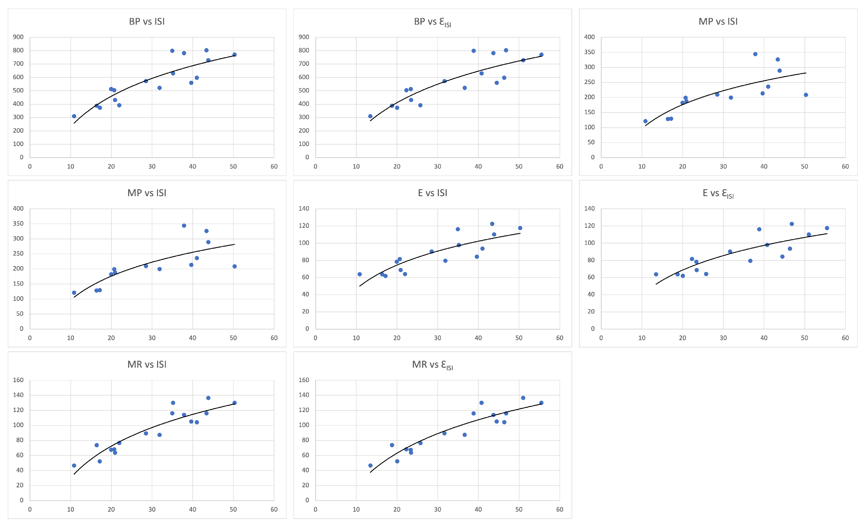
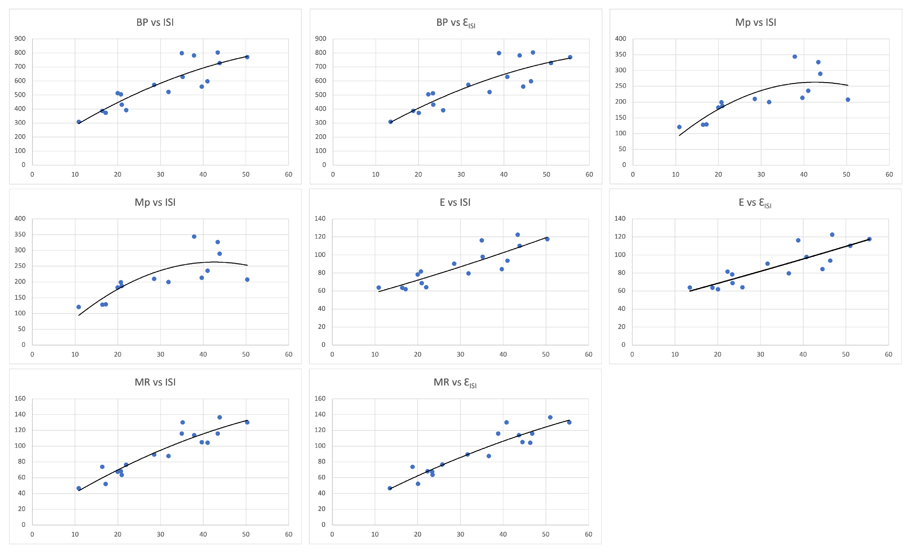
3. Regressions Models and Applications to Anticancer Drugs

We carried out a statistical study to compare the correlation of physicochemical properties and the $ISI$-index (energy) with the chemical structures of anticancer drugs. For the regression models, we considered the most used: linear, logarithmic and quadratic. The picture below displays the molecular structures of various anticancer drugs. Their graph structures can be similarly considered (taking atoms as vertices).

The regression model (linear, logarithmic and quadratic) were

$$\begin{array}{c}\hfill P=a+b(ISI/{\mathcal{E}}_{ISI}),P=aln\left((ISI/{\mathcal{E}}_{ISI})\right)+b,P={(ISI/{\mathcal{E}}_{ISI})}^2+a(ISI/{\mathcal{E}}_{ISI})+b,\end{array}$$

where $a,b$ are constants, and P is the physical property of an anticancer drug. Now, the different linear models’ rounded equations for the $ISI$-index and the $ISI$-energy against physical property of anticancer drug were as follows:

$$\begin{array}{cc}\hfill BP& =12.225ISI+199.18BP=10.963{\mathcal{E}}_{ISI}+193.25Mp=4.0977ISI+88.944\hfill \\ \hfill MP& =3.7228{\mathcal{E}}_{ISI}+85.585E=1.5276ISI+41.632E=1.3656{\mathcal{E}}_{ISI}+41.12\hfill \\ \hfill MR& =2.2757ISI+23.916MR=2.0834{\mathcal{E}}_{ISI}+21.351\hfill \end{array}$$

The scattering of anticancer drugs against their physical properties with the $ISI$-index and the $ISI$-energy via the linear regression model are given in Figure 2.

The different logarithmic model rounded equations for the $ISI$-index and the $ISI$-energy against the physical property of anticancer drug were as follows:

$$\begin{array}{cc}\hfill BP& =329.26ln\left(ISI\right)-527.09,BP=340.56ln\left({\mathcal{E}}_{ISI}\right)-609.11,MP=114.52ln\left(ISI\right)-166.94\hfill \\ \hfill MP& =119.36ln\left({\mathcal{E}}_{ISI}\right)-198.38,E=40.05ln\left(ISI\right)-45.442,E=41.45ln\left({\mathcal{E}}_{ISI}\right)-55.445\hfill \\ \hfill MR& =60.872ln\left(ISI\right)-109.88,MR=64.041ln\left({\mathcal{E}}_{ISI}\right)-128.78\hfill \end{array}$$

The scattering of anticancer drugs with their physical properties against the $ISI$-index and the $ISI$-energy via the logarithmic regression model are given in Figure 3.

The different quadratic model rounded equations for the $ISI$-index and the $ISI$-energy against physical property of anticancer drug were as follows:

$$\begin{array}{cc}\hfill BP& =-0.1409{\left(ISI\right)}^2+20.746ISI+88.239,BP=-0.1285{\mathcal{E}}_{ISI}^2+19.757{\mathcal{E}}_{ISI}+62.688\hfill \\ \hfill MP& =-0.1681{\left(ISI\right)}^2+14.311ISI-41.582,MP=-0.1428{\mathcal{E}}_{ISI}^2+13.534{\mathcal{E}}_{ISI}-57.478\hfill \\ \hfill E& =0.0044{\left(ISI\right)}^2+1.2623ISI+45.087,E=0.0015{\mathcal{E}}_{ISI}^2+1.2624{\mathcal{E}}_{ISI}+42.653\hfill \\ \hfill MR& =-0.0206{\left(ISI\right)}^2+3.5246ISI+7.6566,MR=-0.0132{\mathcal{E}}_{ISI}^2+2.9881{\mathcal{E}}_{ISI}+7.9192\hfill \end{array}$$

The graphical representation of anticancer drugs with their physical properties against the $ISI$-index and the $ISI$-energy in the quadratic regression model are given in Figure 4.

The following table (

Table 1. Various Anticancer Drugs with their Physicochemical Properties and the $ISI$-Index (Energy) of their Chemical Structures.

Drugs	BP	MP	E	MR	$\mathit{ISI}\left(\mathit{G}\right)$	${\mathcal{E}}_{\mathit{ISI}}\left(\mathit{G}\right)$
Amathaspiramide E	572.7	209.72	90.3	89.4	28.5119	31.6741
Aminopterin	782.27	344.45		114	37.85	43.6952
Aspidostomide E	798.8		116.2	116	34.9667	38.8268
Carmustine	309.6	120.99	63.8	46.6	10.85	13.4524
Caulibugulone E	373	129.46	62	52.2	17.1667	20.0501
Convolutamide A	629.9		97.9	130.1	35.1786	40.7735
Convolutamine F	387.7	128.67	63.7	73.8	16.3833	18.7833
Convolutamydine A	504.9	199.2	81.6	68.2	20.7119	22.2929
Daunorubicin	770	208.5	117.6	130	50.2976	55.4943
Deguelin	560.1	213.39	84.3	105.1	39.65	44.5048
Melatonin	512.8	182.51	78.4	67.6	19.9667	23.3733
Minocycline	803.3	326.3	122.5	116	43.3929	46.805
Perfragilin A	431.5	187.62	68.7	63.6	20.9167	23.4653
Podophyllotoxin	597.9	235.86	93.6	104.3	41	46.3479
Pterocellin B	521.6	199.88	79.5	87.4	31.8667	36.6356
Raloxifene	728.2	289.58	110.1	136.6	43.85	51.0142
Tambjamine K	391.7		64.1	76.6	21.9667	25.7574

) gives the physical entities along with the $ISI$-index and the $ISI$-energy. The $BP,MP,E$ and $MR$ were taken from [5]. The $ISI$-index and the $ISI$-energy of these anticancer drugs were calculated by Wolfram Mathematica.

The following tables displays the correlation coefficient of the physicochemical properties of the anticancer drugs with the $ISI$-index and the $ISI$-energy.

From

Table 2. Correlation Coefficients of Anticancer Drugs with the $ISI$-Index (Energy) of their Chemical Structures.

Invariant	BP	MP	E	MR
$ISI\left(G\right)$	0.875742866	0.751128121	0.870072771	0.927336169
${\mathcal{E}}_{ISI}\left(G\right)$	0.865394398	0.752558075	0.853707593	0.935499557

, it can be seen that the $ISI$-index showed a higher significant correlation when compared with other physicochemical properties, while the $ISI$-energy showed a better significant correlation than that of the $ISI$-index when compared with other physicochemical properties

From

Table 3. $R^2$ of Anticancer Drugs with the $ISI$-Index (Energy) of their Chemical Structures.

Linear regression
Invariant	BP	MP	E	MR
$ISI\left(G\right)$	0.7669	0.7489	0.757	0.86
${\mathcal{E}}_{ISI}\left(G\right)$	0.7489	0.5663	0.7288	0.8752
Logarithmic regression
Invariant	BP	MP	E	MR
$ISI\left(G\right)$	0.7672	0.6064	0.7141	0.8484
${\mathcal{E}}_{ISI}\left(G\right)$	0.7553	0.6066	0.6994	0.8642
Quadratic regression
Invariant	BP	MP	E	MR
$ISI\left(G\right)$	0.777	0.6497	0.7576	0.867
${\mathcal{E}}_{ISI}\left(G\right)$	0.7599	0.6454	0.7289	0.8789

, the coefficient of determination ($R^2$) was again better for the molar refraction $MR$; however, $R^2$ was higher for the $ISI$-energy than for the $ISI$-index for the molar refraction of the anticancer drugs.

From Table 2 and Table 3 along with the pictures, it can be concluded that the correlations of all the physicochemical properties of anticancer drugs with the $ISI$-index (energy) were highly significant. Further, the study implied that these anticancer drugs may be considered for designing new drugs using the $ISI$-index (energy) and other related topological indices. As the regression analysis showed a high correlation of the $ISI$-index (energy) for these drugs, their combination may be considered for novel drugs.

4. Conclusions

This study showed that the physicochemical properties of anticancer drugs can be treated by certain topological indices such as the $ISI$-index and the $ISI$-energy in this report. We observed that the physical and chemical properties of anticancer drugs were well correlated with such topological indices. Moreover, this work implied that these anticancer drugs may be utilized for further study by pharmacists and chemists in designing new drugs, using the concept of these topological indices. The more correlated drugs may have a better impact on the treatment of cancer. For a better treatment of cancer, a future study may be carried out by interdisciplinary researchers as a joint venture.

References

1. Havare, O.C. The inverse sum indeg index (ISI) and ISI-energy of Hyaluronic Acid-Paclitaxel molecules used in antiancer drugs. Open J. Discret. Appl. Math. 2021, 4, 72–81. [Google Scholar] [CrossRef]
2. Hernández, J.C.; Rodríguez, J.M.; Sigarreta, J.M. The geometric-arithmetic index by decompositions-CMMSE. J. Math. Chem. 2017, 55, 1376–1391. [Google Scholar] [CrossRef]
3. Hosamani, S.M.; Kulkarni, B.B.; Boli, R.G.; Gadag, V.M. QSPR analysis of certain graph theoretical matrices and their corresponding energy. Appl. Math. Nonlinear Sci. 2017, 2, 131–150. [Google Scholar] [CrossRef] [Green Version]
4. Kirmani, S.A.K.; Ali, P.; Azam, F.; Alvi, P.A. On Ve-Degree and Ev-Degree Topological Properties of Hyaluronic Acid? Anticancer Drug Conjugates with QSPR. J. Chem. 2021, 2021, 3860856. [Google Scholar] [CrossRef]
5. Shanmukha, M.C.; Basavarajappa, N.S.; Shilpa, K.C.; Usha, A. Degree-based topological indices on anticancer drugs with QSPR analysis. Heliyon 2020, 6, e04235. [Google Scholar] [CrossRef] [PubMed]
6. Rather, B.A.; Aouchiche, M.; Imran, M.; Pirzada, S. On arithmetic–geometric eigenvalues of graphs. Main Group Met. Chem. 2022, 45, 111–123. [Google Scholar] [CrossRef]
7. Cvetković, D.M.; Rowlison, P.; Simić, S. An Introduction to Theory of Graph Spectra; London Mathematical Society Student Texts, 75; Cambridge University Press: Cambridge, UK, 2010. [Google Scholar]
8. Brouwer, A.E.; Haemers, W.H. Spectra of Graphs; Springer: New York, NY, USA, 2010. [Google Scholar]
9. Gutman, I. The Energy of a graph. Ber. Math. Statist. Sekt. Forsch-Ungszentram Graz. 1978, 103, 1–22. [Google Scholar]
10. Gutman, I. Topology and stability of conjugated hudrocarbons. The dependence of total π-electron energy on molecular topology. J. Serb. Chem. Soc. 2005, 70, 441–456. [Google Scholar] [CrossRef]
11. Nikiforov, V. Beyond graph energy: Norms of graphs and matrices. Linear Algebra Appl. 2016, 506, 82–138. [Google Scholar] [CrossRef] [Green Version]
12. Rather, B.A.; Imran, M. A note on the energy and Sombor energy of graphs. MATCH Commun. Math. Comput. Chem. 2023, 89, 467–477. [Google Scholar] [CrossRef]
13. Filipovski, S.; Jajcay, R. Bounds for the energy of graphs. Mathematics 2021, 9, 1687. [Google Scholar] [CrossRef]
14. Li, X.; Shi, Y.; Gutman, I. Graph Energy; Springer: New York, NY, USA, 2012. [Google Scholar]
15. Vukiećevixcx, D. Bond additive modeling 2. Mathematical properties of max-min rodeg index. Croat. Chem. Acta 2010, 83, 261–273. [Google Scholar]
16. Nezhad, F.F.; Azari, M.; Došlić, T. Sharp bounds on the inverse sum indeg index. Discret. Appl. Math. 2017, 217, 185–195. [Google Scholar] [CrossRef]
17. Zangi, S.; Ghorbani, M.; Eslampour, M. On the eigenvalues of some matrices based on vertex degree. Iran. J. Math. Chem. 2018, 9, 149–156. [Google Scholar]
18. Hafeez, S.; Farooq, R. Inverse sum indeg energy of graphs. IEEE Acess 2019, 7, 100860–100866. [Google Scholar] [CrossRef]
19. Bharali, A.; Mahanta, A.; Gogoi, I.J.; Doley, A. Inverse sum indeg index and ISI-matrix of graphs. J. Discret. Math. Sci. Cryptogr. 2020, 23, 1315–1333. [Google Scholar] [CrossRef]
20. Li, F.; Li, X.; Broersma, H. Spectral properties of inverse sum indeg index of graphs. J. Math. Chem. 2020, 58, 2108–2139. [Google Scholar] [CrossRef]
21. Li, F.; Ye, Q.; Broersma, H. Some new bounds for the inverse sum indeg energy of graphs. Axioms 2022, 11, 243. [Google Scholar] [CrossRef]
22. Zou, X.; Rather, B.A.; Imran, M.; Ali, A. On Some Topological Indices Defined via the Modified Sombor Matrix. Molecules 2022, 27, 6772. [Google Scholar] [CrossRef]
23. Jamaal, F.; Imran, M.; Rather, B.A. On inverse sum indeg energy of graphs. Spec. Matrices 2022, 10, 1–10. [Google Scholar] [CrossRef]
Figure 1. Molecular Structures of Certain Anticancer Drugs.
Mathematics 10 04749 g001
Figure 2. Linear Regression for Physical Property with the I S I -index and E I S I of Anticancer Drugs.
Mathematics 10 04749 g002
Figure 3. Logarithmic Regression for Physical Property with the I S I -index and E I S I of Anticancer Drugs.
Mathematics 10 04749 g003
Figure 4. Logarithmic Regression for Physical Property with the I S I -index and E I S I of Anticancer Drugs.
Mathematics 10 04749 g004