Article

Bayesian Inference Algorithm for Estimating Heterogeneity of Regulatory Mechanisms Based on Single-Cell Data

1
School of Mathematics and Statistics, Central China Normal University, Wuhan 430079, China
2
School of Statistics and Mathematics, Zhongnan University of Economics and Law, Wuhan 430073, China
3
School of Mathematics, Monash University, Clayton, VIC 3800, Australia
*
Authors to whom correspondence should be addressed.
Mathematics 2022, 10(24), 4748; https://doi.org/10.3390/math10244748
Submission received: 27 October 2022 / Revised: 5 December 2022 / Accepted: 7 December 2022 / Published: 14 December 2022
(This article belongs to the Special Issue Recent Advances in Computational Statistics)

Abstract

:
The rapid progress in biological experimental technologies has generated a huge amount of experimental data to investigate complex regulatory mechanisms. Various mathematical models have been proposed to simulate the dynamic properties of molecular processes using the experimental data. However, it is still difficult to estimate unknown parameters in mathematical models for the dynamics in different cells due to the high demand for computing power. In this work, we propose a population statistical inference algorithm to improve the computing efficiency. In the first step, this algorithm clusters single cells into a number of groups based on the distances between each pair of cells. In each cluster, we then infer the parameters of the mathematical model for the first cell. We propose an adaptive approach that uses the inferred parameter values of the first cell to formulate the prior distribution and acceptance criteria of the following cells. Three regulatory network models were used to examine the efficiency and effectiveness of the designed algorithm. The computational results show that the new method reduces the computational time significantly and provides an effective algorithm to infer the parameters of regulatory networks in a large number of cells.

1. Introduction

The fast progress in biological experimental technologies in recent years has generated a huge amount of experimental data to investigate the molecular regulatory mechanisms inside the cell [1,2,3,4]. Among them, single-cell technologies have been used to quantify the expression profiles and protein activities in different single cells at the same time [5,6]. These quantitative and qualitative datasets provide rich information for studying the heterogeneity of regulatory mechanisms in different cells and in different patients for disease therapy. However, there are substantial challenges in illustrating the origin of heterogeneity and to describe the propagation of heterogeneity in cellular processes [7,8].
Mathematical modeling is a powerful method to investigate the diverse dynamic observations in a large number of cells. For time-lapse data, the two-stage modeling method uses a single mathematical model with different model parameter values to simulate the diverse dynamics in single cells [9]. The heterogeneity of biological processes is demonstrated by the distributions of the model parameters, which may be overestimated. To address this issue, the global two-stage method uses a local measure for the distributions of the model parameters [10]. Another widely used method is the mixed-effect model, which derives the likelihood functions of the model parameters by employing the first-order conditional estimation [11,12] or the stochastic approximation expectation–maximization algorithm [11]. In addition, the maximum entropy method has been used to analyze the single-cell snapshot data [13]. Furthermore, the likelihood function has been used to identify the variability in biological processes and the distributions of the model parameters [14,15]. More related research studies can be found in the review articles published in recent years [16,17].
In this study, we discuss inference methods for estimating the unknown model parameters based on single-cell time-lapse data. Thus, we estimate a number of mathematical models using the same model equations, but with different sets of model parameters. For the inference of the unknown model parameters, the Bayesian statistical methods and optimization algorithms are two major types of widely used methods [18,19,20]. In recent years, machine learning methods have been used to estimate unknown model parameters [21]. Among these methods, the Bayesian inference methods are able to obtain the distributions of the model parameters and also have the ability to analyze noisy datasets with better accuracy. However, the classic Markov chain Monte Carlo (MCMC) method needs the likelihood function to assess the accuracy of the model parameters, which are difficult to apply to complex systems without explicit likelihood functions. To overcome this limitation, the approximate Bayesian computation (ABC) algorithms have been proposed to measure the accuracy of the model parameters by comparing the model simulations with experimental data directly [22]. The first proposed ABC was the ABC rejection algorithm, which needs a large computing time because this method has no learning step. More effective algorithms have been designed to speed up the convergence rate, for example ABC-MCMC and sequential Monte Carlo (SMC) ABC [23,24,25]. In recent year, more measures have been designed to assess the accuracy of the model simulations [26]; the early rejection algorithms have been developed to reduce the computing time [27].
The ABC-SMC algorithm uses the adaptive transitional kernel functions to accelerate the acceptance rate [24]. However, this may be difficult for the model solutions close to the experimental data if the data are noisy. Thus, the selection of the tolerance threshold values is critical for the successful applications of ABC-SMC. One option for selecting the threshold values is to use the simulation errors of the accepted samples to construct the adaptive tolerance threshold [23,28]. However, it is not easy to use these adaptive approaches to estimate the model parameters using noisy data. For the application problems, a simple approach is to choose the threshold values by manual adjustment. Since the single-cell time-lapse datasets may include observations from a large number of single cells, it is not practical to adjust the threshold values for each single cell.
We conducted initial computations to infer the parameters in a population of models [29]. This study used the existing ABC-SMC to infer the parameters of each model, which requires a huge computing time. To address the identified challenges in our initial study, we designed a new algorithm in this work to reduce the computational time of ABC-SMC. The innovation of this study is dividing the dataset with many single cells into a few clusters. Each cluster has a number of single cells whose expression profiles are close to each other. After obtaining the estimates of the parameters for the first cell in each cluster, we designed an adaptive method to use these estimates to construct the threshold values for the other cells in the same cluster. Three test system models were used to evaluate the efficiency of the proposed algorithm.

2. Materials and Methods

2.1. Mathematical Model

In this work, we studied the inference methods for estimating the unknown parameters of the following system:
d x i d t = f i ( x 1 , x 2 , , x n , B 1 , B 2 , , B m ) , i = 1 , 2 , , n ,
where ( x 1 ( t ) , , x n ( t ) ) are the system states at time t, ( B 1 , , B m ) are model parameters, and functions ( f 1 , , f n ) describe the evolutions of the system state. If the value of B i ( i = 1 , , m ) is constant, System (1) is the traditional ordinary differential equations (ODEs). Here, we studied the case that B i are random variables following a joint distribution. Note that, unlike stochastic differential equations, the value of B i is not a sample of a stochastic process over time. To simulate the dynamics in single cells, it was assumed that the model for each single cell has a particular value of parameter B i , and the model of different single cells has different values. These values are samples of the particular joint distribution.
In the inference study, we first generated a sample of parameters ( b 1 , , b m ) from a prior distribution π ( θ ) . Since we did not have any information about the prior distribution, it was assumed that this distribution is a uniform distribution over the interval [ a , b ] . The values of a and b are selected in the inference steps. In addition, it was assumed that random variables B i are independent of each other. Once a sample ( b 1 , , b m ) is obtained, we used the differential equation system (1), in which random variable B i is replaced by sample b i , to simulate the molecular dynamics in single cells.

2.2. Approximation Bayesian Computation

This subsection briefly introduces the widely used ABC-SMC algorithm, which was used in this work to infer the model parameters. We also discuss the issues in the applications of this algorithm, which is given below [30]. More detailed information regarding the implementations of this algorithm can be found in [22].
The discrepancy between the simulation and experimental data is the mean-squared relative error, calculated by
ρ ( X , Y ) = 1 m T i = 1 m j = 0 T x i j y i j x i j 2 ,
where y i j and x i j are the experimental data and model simulation of the i-th variable x i at time point t j , respectively.
One question in the application of ABC-SMC is the choice of the proper threshold values ϵ 1 , , ϵ K . Although we may be able to manually select these values for the experimental data in each single cell, it is time consuming to choose these values manually when the cell number is large. Thus, we needed to design a technique to select the threshold values effectively for a large number of cells.

2.3. ABC-SMC with Adaptive Tolerance Threshold

To improve the efficiency, a natural idea is to use the estimated parameters for the first cell to construct the threshold values and prior distribution for the cell that is close to the first cell. We can use particles in the last generation (i.e., the K-th generation in Algorithm 1) to develop the prior distribution and use the corresponding discrepancies in Step 3.4 in Algorithm 1 to design the tolerance threshold.
Algorithm 1 ABC-SMC algorithm.
1:
Input information: experimental data X = { x 0 , x 1 , , x T } at time point t = [ t 0 , t 1 , , t T ] ; prior distribution of parameters π ( θ ) , tolerance threshold values ϵ 1 , , ϵ K , where K is the number of generations.
2:
The first generation k = 1
  • For particle j = 1 , , M
       (1)
    Use the prior distribution to generate a sample θ * π ( θ ) .
       (2)
    Simulate the model with parameters θ * to obtain the simulation data X * Model( θ * ).
       (3)
    Calculate the discrepancy between simulation data and experimental data ρ ( X , X * ) .
       (4)
    If ρ ( X , X * ) > ϵ 1 , reject the sample. Otherwise, accept this sample as θ j , 1 = θ * .
       (5)
    Set the same weight to each particle as w j , 1 = 1 M .
  • Set the variance of the particles in the first generation σ k 2 = 2 V a r ( θ 1 : M , 1 ) .
3:
For generations k = 2 , , K
  • For particle j = 1 , , M :
       (1)
    Based on the accepted samples in the previous generation, select a sample θ * using the weights of the previous generation w 1 : M , k 1 .
       (2)
    Generate a new sample θ * * q ( θ | θ * , σ k 1 ) using the proposed distribution.
       (3)
    Simulate the model with parameter θ * * to obtain the simulation data X * * Model( θ * * ).
       (4)
    Calculate the discrepancy between the simulation data and experimental data ρ ( X , X * * ) .
       (5)
    If ρ ( X , X * * ) > ϵ k , reject the sample. Otherwise, accept this sample as θ j , k = θ * * .
  • Calculate the new weights for the accepted samples in generation k:
       (1)
    The new weight is w j , k = π ( θ j , k ) i = 1 M w i , k 1 q ( θ i , k | θ j , k , σ k 1 ) .
  • The new variance is σ k 2 = 2 V a r ( θ 1 : M , k ) .
4:
Output: the accepted samples in the K-th generation θ 1 : M , K and the corresponding discrepancies ρ 1 : M , K .
However, this idea cannot be applied directly if the experimental data in two cells have a large distance. For example, these two cells may belong to different cell types, or they may be at different developmental stages. Mathematically, the observed dynamics may show different trends. In addition, after obtaining the estimated parameters for a number of cells, we need to select an optimal estimate to match the dynamics of the next cell.
To address these issues, two improvements of Algorithm 1 are proposed in this work. First, we divided all observed cells into a number of clusters based on the distance between each pair of cells. Since we needed to develop the initial information (i.e., the prior distribution and threshold values) for the first cell in each cluster, the cluster number should not be very small (i.e., the difference between cells in one cluster may be large) or very large (i.e., computational inefficiency). In this study, the cluster number for the three test systems was selected in the range between 10 and 15, depending on the variations of the observations in the dataset.
We first used the mean values of all cells in each cluster to determine the centroid of that cluster and then found the first cell that had the smallest distance to the cluster centroid. Alternatively, we can use medoid clustering for grouping cells and determining the first cell. In medoid clustering, we chose an actual data point as the centroid of a cluster. This is different from the k-means clustering, which uses the mean values as the centroid of a cluster. Based on the first cell, we ranked all the cells in this cluster based on their distances to the first cell. We first used Algorithm 1 to infer the unknown parameters of the first cell, which were then employed to determine the initial information of the second cell. For the k-th cell ( k > 2 ), we found a cell from the cells 1 , 2 , , k 1 that has the smallest distance to the k-th cell and, then, used the estimated parameters of that cell to determine the initial information of the k-th cell.
Except for the first cell, the prior distribution of each parameter θ i was assumed to follow the uniform distribution π ( θ ) U ( W m i n , W m a x ) . Assume that the estimated values of this parameter in the previous cell are θ K , i in the final K-th generation. The boundaries of the uniform distribution are
W m i n = k 1 min { θ 1 : M , K } , W m a x = k 1 max { θ 1 : M , K } ,
where parameter k 1 is associated with the distance between these two cells. For the tolerance threshold, using the M discrepancy values ρ 1 : M , K in the final generation of the previous cell, we set the first tolerance threshold as
ϵ 1 = k 2 max { ρ 1 : M , K } ,
where parameter k 2 is associated with the distance between these two cells. For the following generations, we used the discrepancy values of the previous generation to determine the tolerance threshold adaptively. The major steps of the proposed method are given in Algorithm 2.
Algorithm 2 ABC-PMC with adaptive tolerance threshold (ABC-CPMC).
1:
Initiation: observation data X = { X 1 , X 2 , , X N } of N cells.
2:
Cluster these N cells into C clusters, and find the centroid of each cluster. Each cluster has N i cells ( i = 1 , , C ).
3:
For clusters i = 1 , , C :
(1)
Based on the centroid X i * of this cluster, find the first cell of this cluster by min j ρ ( X i j X i * ) ( j = 1 , , N i ). Denote the data of the first cell as X i 1 .
(2)
Rank all N i cells in the i-th cluster as X i 1 , X i 2 , , X i N i based on their distances from the first cell.
(3)
For the first cell X i 1 , use Algorithm 1 and prior θ * π ( θ ) to infer the model parameters. Denote the inferred parameter as θ 1 : M , K i 1 .
(4)
For the second cell X i 2 , construct the prior as θ * U ( a , b ) using Formula (3). The tolerance threshold ϵ 1 is determined by using Formula (4).
(5)
Use Algorithm 1 to estimate the parameters θ 1 : M , K i 2 of the second cell.
(6)
For cells k = 3 , , N i :
(a)
Find a cell from the cells 1 , 2 , , k 1 that has the smallest distance to the k-th cell in these k 1 cells. Denote the particles in the final generation of this cell as θ 1 : M , K i ( k 1 ) * .
(b)
Construct the prior as θ * U ( a , b ) using Formula (3). The tolerance threshold ϵ 1 is determined by using Formula (4).
(c)
Use Algorithm 1 to estimate the parameters θ 1 : M , K i k of the k-th cell.
Note that we can also use the proposed technique in Algorithm 2 for ranking cells in a cluster in Steps 3.1 and 3.2 to rank all clusters based on the centroid of each cluster. In this way, the prior distribution of the first cell in a cluster may be obtained by the estimated parameters of the neighboring cluster.

3. Results and Discussion

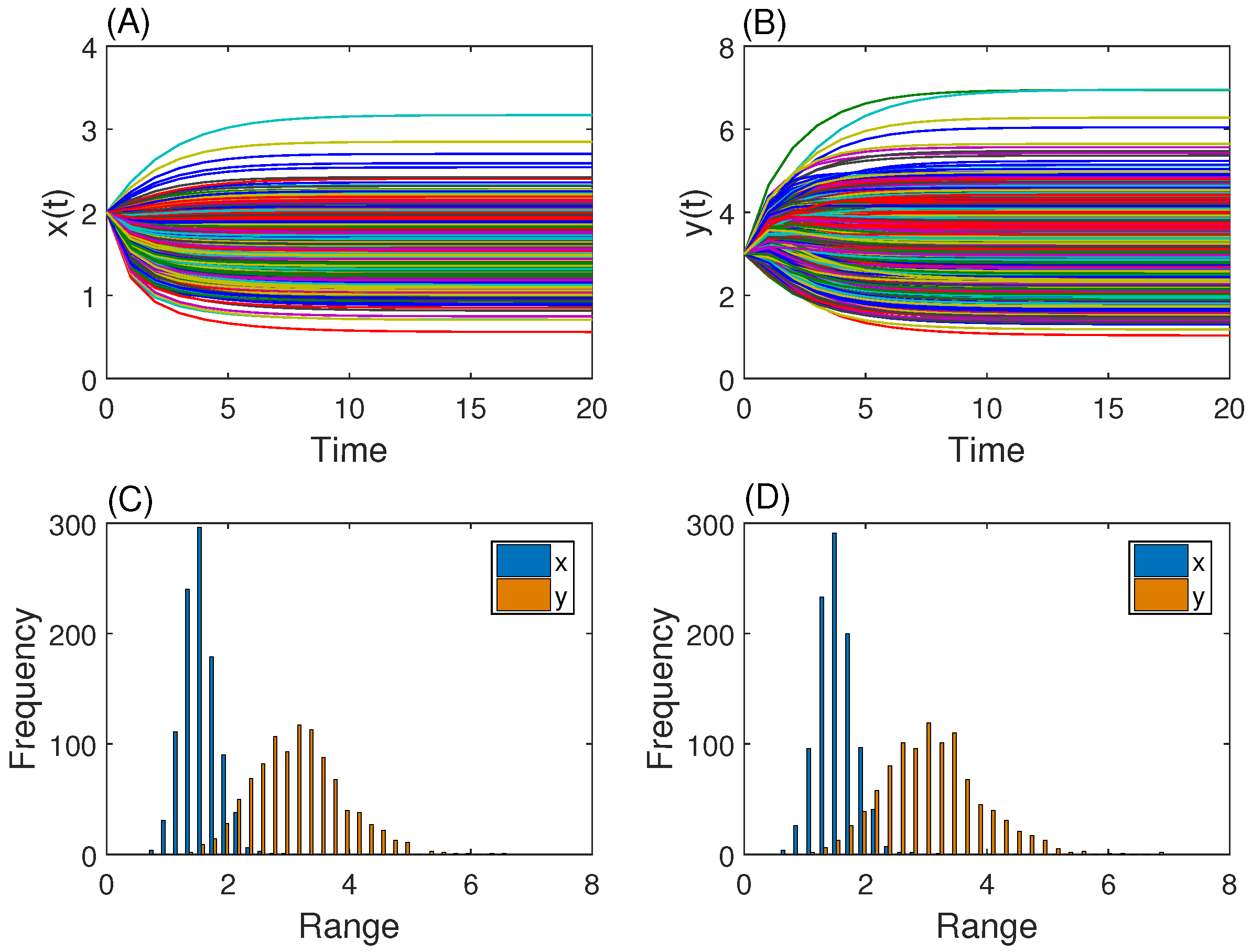
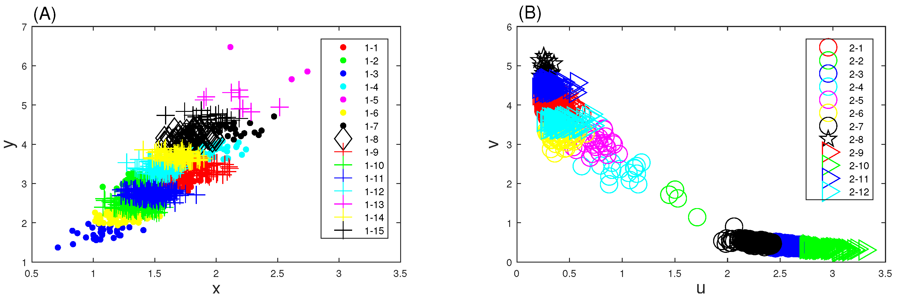
3.1. Gene Network with One Steady State

We first considered a mathematical model for studying the dynamics of a single gene [31]. This gene has a positive regulation of itself, and this regulation is described by a Michaelis–Menten function. The produced mRNA ( x ) from the first equation below will synthesize the proteins ( y ) in the second equation. The model is given by
d x d t = a y 1 + y k 1 x , d y d t = b x k 2 y ,
where a and k 1 are the synthesis rate and degradation rate of the mRNA and b and k 2 are the synthesis rate and degradation rate of the protein, respectively. These four rates are assumed to follow the Gaussian distributions, namely a and b N ( 2 , 1 ) , as well as k 1 and k 2 N ( 1 , 0.5 2 ) . We used a fixed initial condition: ( x 0 , y 0 ) = ( 2 , 3 ) .
We tested this system by using 500 simulations [29]. In this study, we extended the simulation number to 1000, shown in Figure 1. Since a Gaussian distribution may generate samples with a wide range of values, we restricted the samples values of a and b in the interval ( 1 , 3 ) and those of k 1 and k 2 in the interval ( 0.5 , 1.5 ) . In addition, simulations with large outliers (i.e., x > 3.5 or y > 7 ) were removed.
We first divided the 1000 generated simulations in Figure 1 into 15 clusters using the command kmeans.m in MATLAB. The number of cluster was selected to avoid mixing the cells in different groups. The minimal distance from cells outside a cluster to the centroid of that cluster is larger than the maximal distance from cells inside the cluster to their centroid. For each simulation, we averaged the values of x and y over the 21 observation time points (i.e., t = 0 , 1 , , 20 ) and, then, drew the scatter plot of these 1000 simulations in Figure 2A. This shows that the simulations of the same cluster have small distances to each other. All the clusters are connected, and Clusters 3 and 5 are located at the two ends of the spectrum. Note that this figure gives a two-dimensional representation of the 21-dimensional data. The mixture of the points in the figure does not mean these points mix in the two-dimensional space.
When inferring the unknown parameters, the prior distribution was assumed to be a uniform distribution π ( θ ) U ( W m i n , W m a x ) for each parameter for the first cell in each cluster. The values of W m i n and W m a x are ( 1 , 1 , 0.5 , 0.5 ) and ( 3 , 3 , 1.5 , 1.5 ) for ( a , b , k 1 , k 2 ) , respectively. The tolerance threshold values ϵ i ( i = 1 , , 10 ) were selected manually as small as possible for the first cell.
Figure 3 provides the simulated frequencies of the estimated parameters and those of the exact parameters of Model (5). The simulated distributions have very good accuracy with respect to the exact ones. However, the variances of the inferred distributions are larger than those of the exact ones because the prior distributions were assumed to be the uniform distributions. The simulated frequencies can be used as the posterior distributions for further analysis.

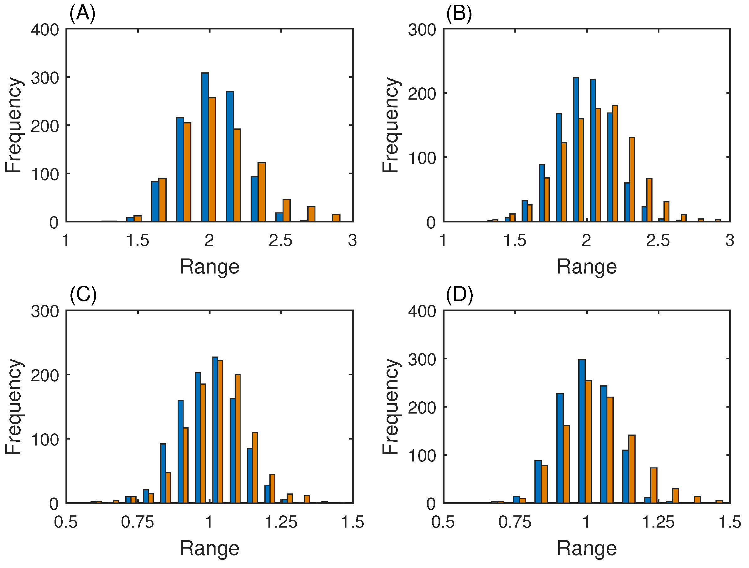
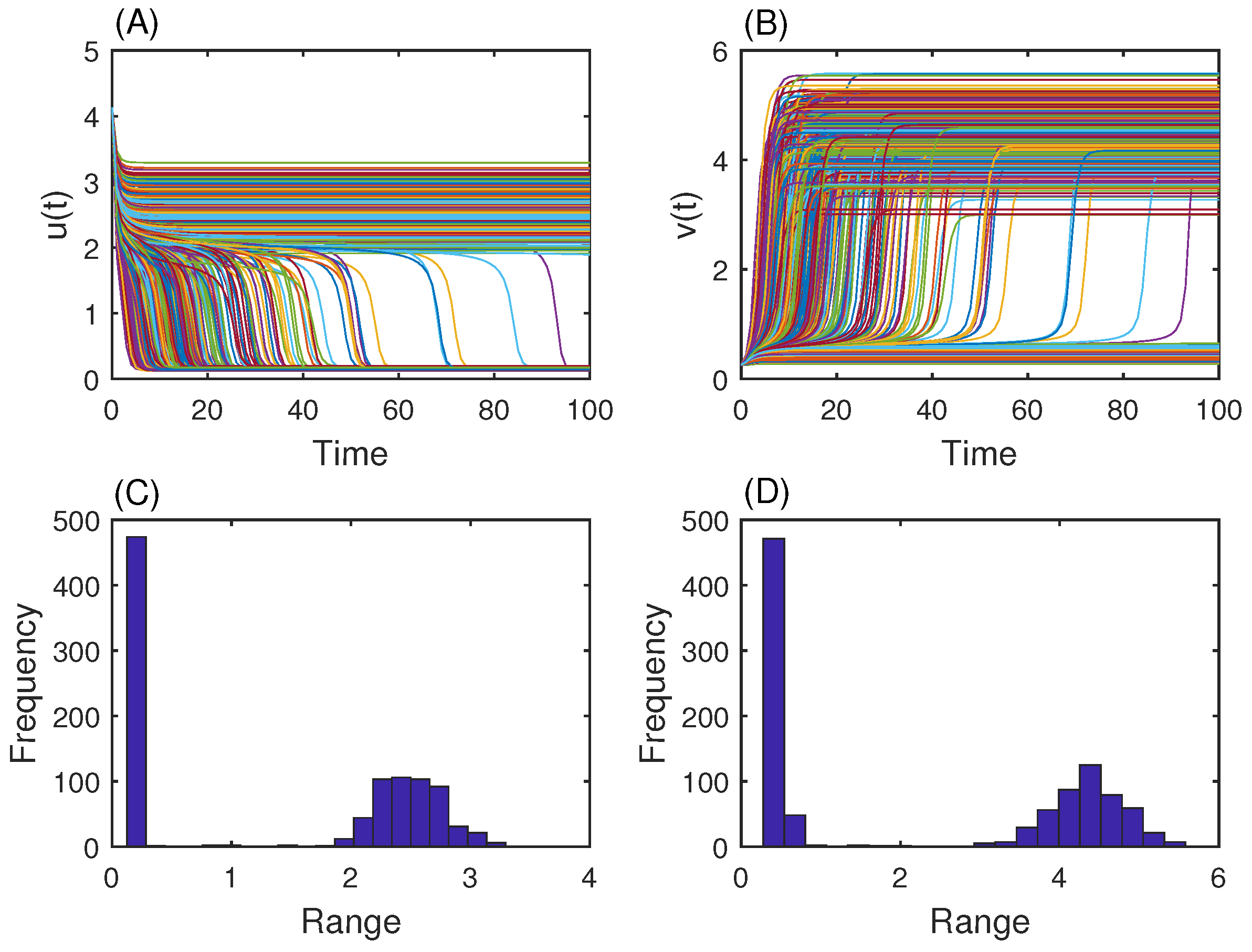
3.2. Genetic Toggle Switch Showing Bistability

The second test system is the genetic toggle switch model for the expression of the two genes [31,32]. The repressor genes λ CI (u) and LacR (v) negatively regulate the other gene. The mathematical model is given by
d u d t = α 1 + β 1 1 + v 3 1 + s 1 + s u , d v d t = α 2 + β 2 1 + u 3 v ,
where α 1 and α 2 are the rate constants of the basal synthesis of the two genes and β 1 and β 2 are the rate constants to realize the negative regulations from the other gene, and s is used to realize genetic switching regulated by protein RecA.
We tested this model (6) by using 500 simulations [29]. In this study, we extended the simulation number to 1000, shown in Figure 1. The fixed initial condition was ( u 0 , v 0 ) = ( 4.1341 , 0.2558 ) . The system parameters were assumed to obey Gaussian distributions, namely α 1 , α 2 N ( 0.2 , 0.01 2 ) , β 1 , β 2 N ( 4 , 0.5 2 ) , and s N ( 2.135 , 0.1 2 ) . This model shows two steady states, but each simulation has only one of these two stable states. The distributions of the steady states at t = 50 obtained by different model parameters are given in Figure 4C,D.
We first divided the 1000 generated simulations in Figure 1 into 12 clusters using kmeans.m in MATLAB. Similar to the first test system, the number of cluster was selected to avoid mixing the cells in different groups. For each simulation, we averaged the values of u and v over the 101 observation time points (i.e., t = 0 , 1 , 2 , , 100 ) and, then, drew the scatter plot of these 1000 simulations in Figure 2B. The two separate groups of clusters are clearly shown, which indicates the two stable steady states of the system. This result suggests the importance of clustering. When a population of cells has different cell types, the cellular dynamics may be distinct in different cell types. Figure 2B clearly gives the characterization of the bistability property of the gene network. We can use different initial information to estimate the unknown parameters for the cells in these two groups.
Based on the clusters shown in Figure 2B, we next inferred the model parameters for each cell using our proposed algorithm. For the first cell of each cluster, the tolerance threshold values of 10 generations were set as ϵ = { 1 , 0.5 , 0.1 , 0.05 , 0.01 , 0.005 , 0.002 , 0.001 , 0.0005 , 0.0002 } initially.
Figure 5 provides the simulated frequencies of estimated parameters and those of the exact parameters of Model (6). Figure 5B–D show that the simulated distributions have very good accuracy with respect to the exact ones for β 1 , α 2 and β 2 . However, Figure 5A suggests that the accuracy of the estimates for parameter s is not as good as those of the other three parameters. The reason for this low accuracy may be that parameter s is not zero only in a short time period. The simulated frequencies can be used as the posterior distributions for further analysis.

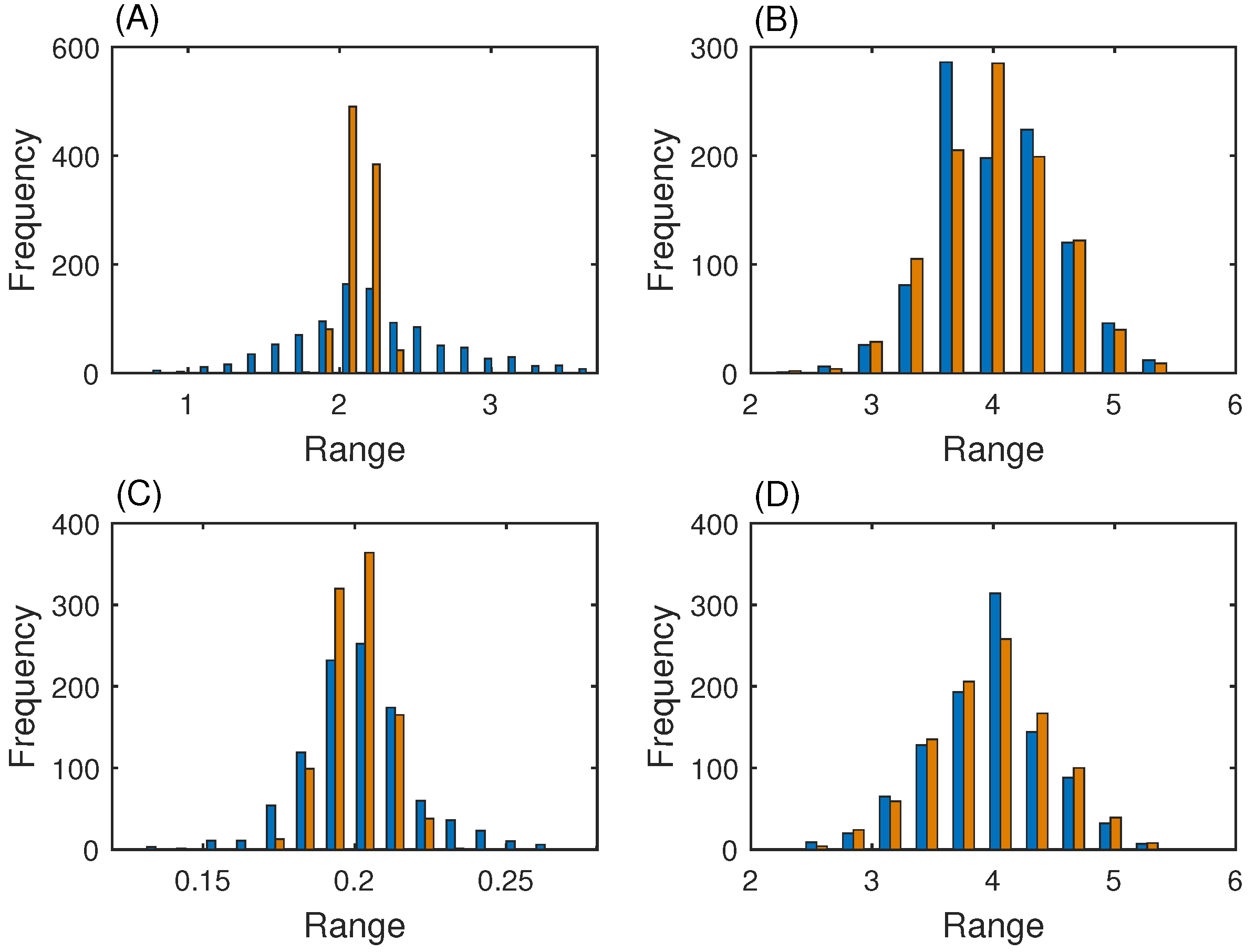
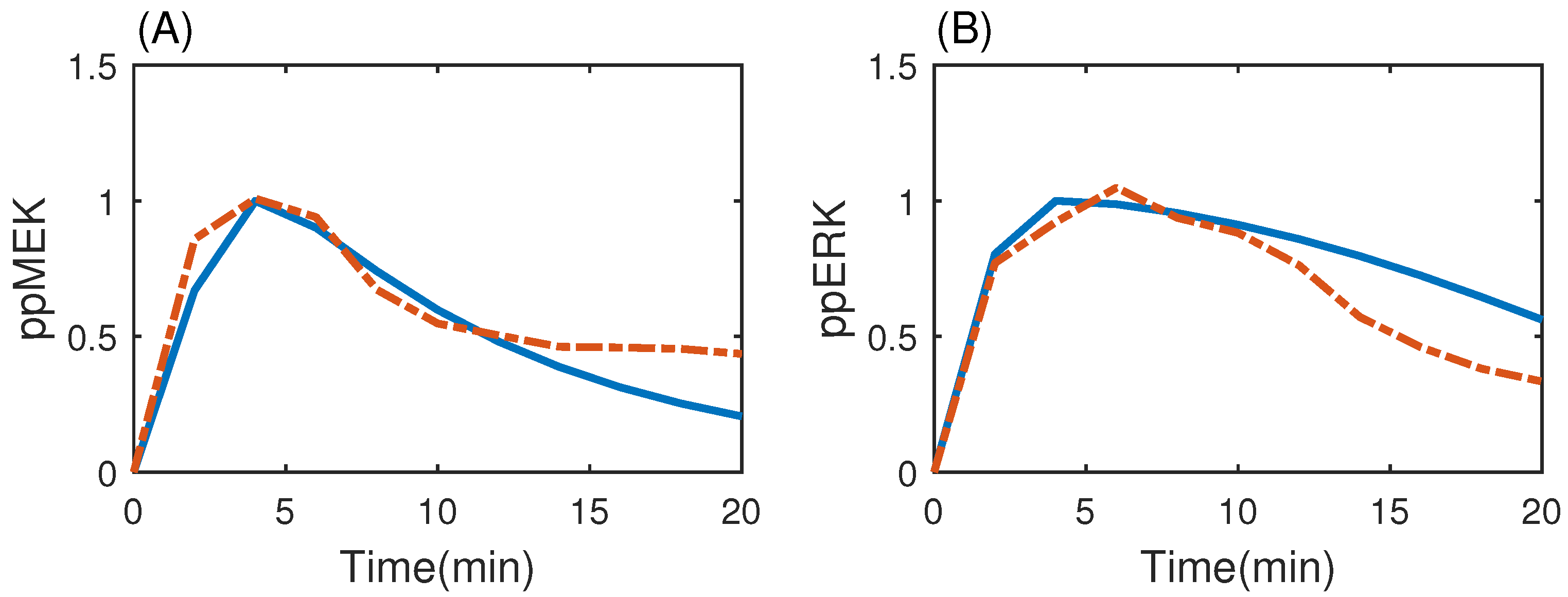
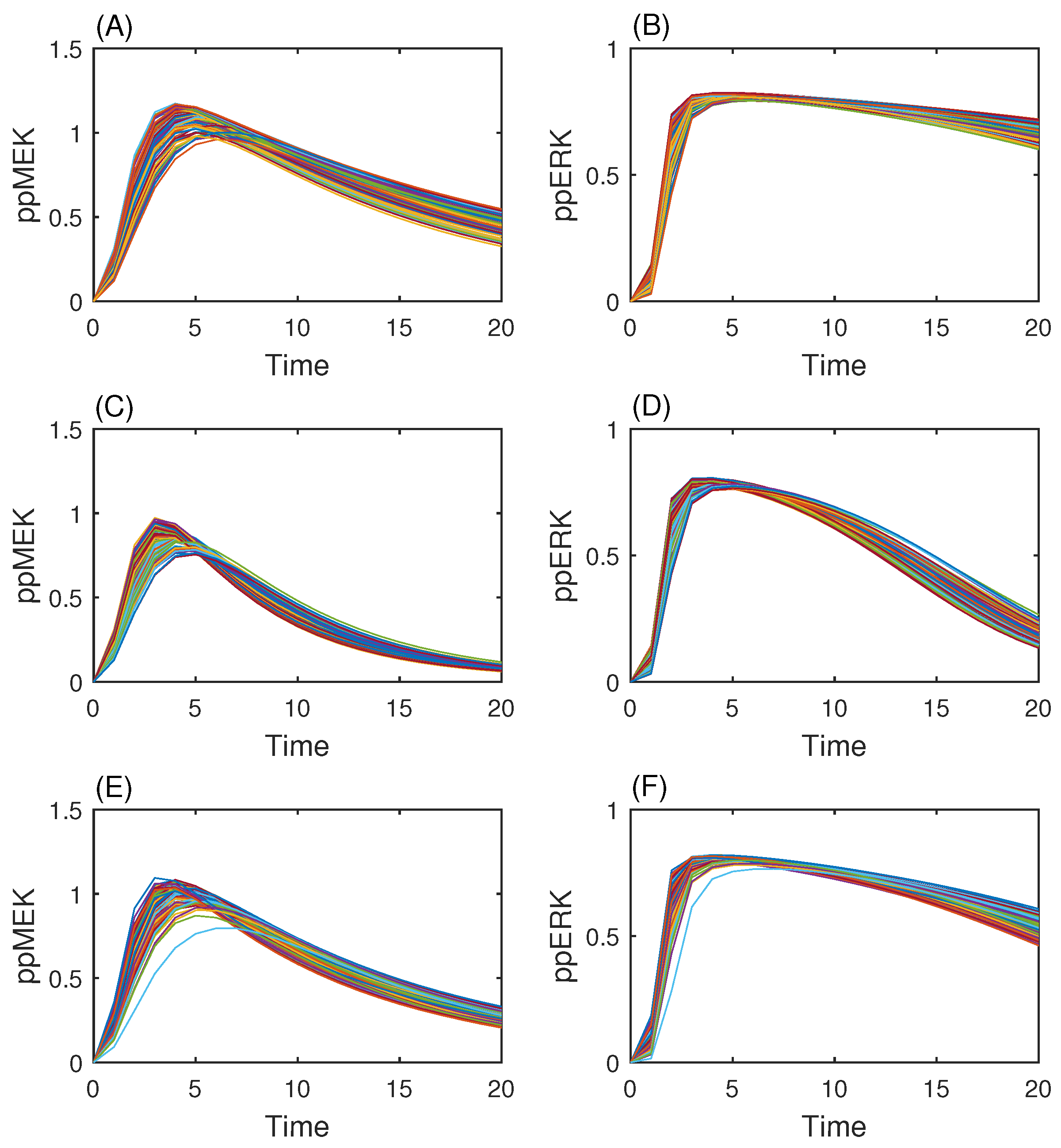
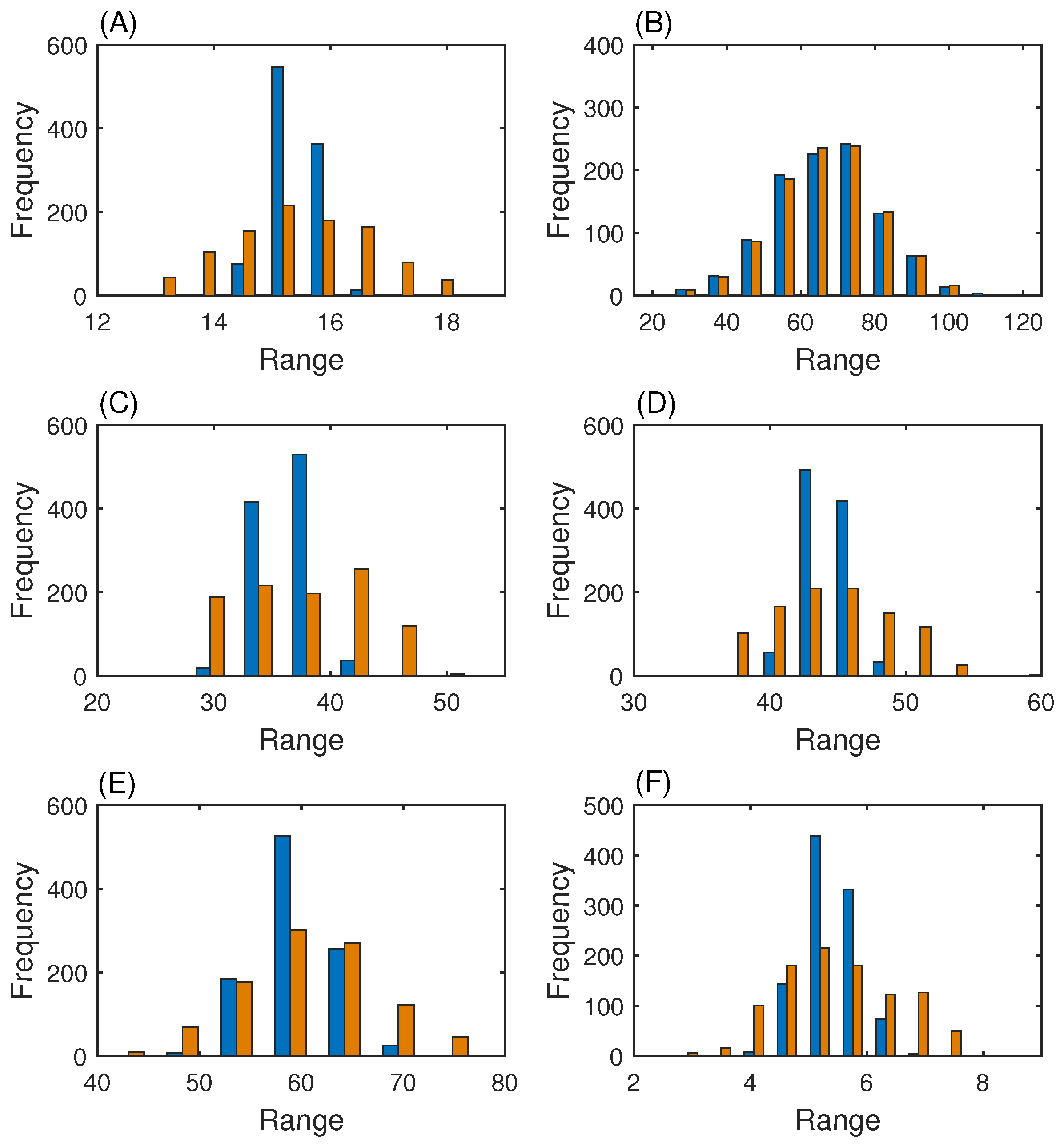
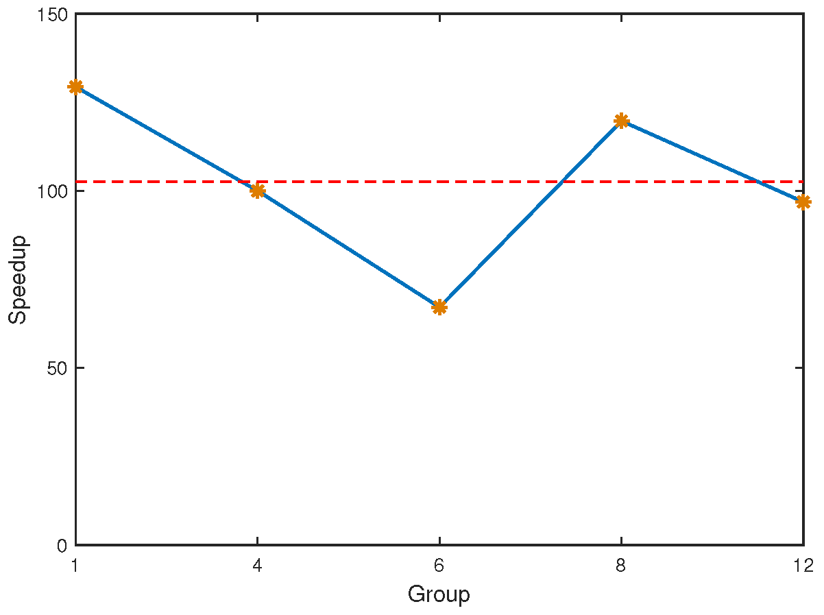
3.3. MAP Kinase Pathway for Efficiency Test

We tested the accuracy of our proposed algorithm by using two small-scale models of genetic regulations. The key question is whether the new method can achieve substantial improvement of the efficiency over the existing methods. To answer this question, we next considered the mathematical model of the MAP kinase pathway, which is one of the most prominent components of the pathways that control cell proliferation, differentiation, and apoptosis. Based on the observation data in single cells, this work studied a subnetwork of the MAP kinase pathway using the activated Raf protein as the input [14]. The activated Raf protein, denoted as pRaf, activates MEK proteins by phosphorylation, leading to double-phosphorylated MEK (ppMEK). The activated MEK protein then activates the ERK proteins by phosphorylation, leading to single-phosphorylated ERK (pERK) and double-phosphorylated ERK (ppERK). Meanwhile, the phosphatases MEK-P’ase (MEKP) and ERK-P’ase (ERKP) can deactivate ppMEK and ppERK, respectively [33,34]. The detailed process of the kinase activations consists of seven sets of biochemical reactions [35], which are given below. The detailed model of the ODEs is provided in the Supplementary Materials.
R 1 : pRaf + MEK d 1 a 1 pRaf − MEK k 1 pRaf + ppMEK,
R 2 : ppMEK + MEKP d 2 a 2 ppMEK − MEKP k 2 pMEK + MEKP,
R 3 : pMEK + MEKP d 3 a 3 pMEK − MEKP k 3 MEK + MEKP,
R 4 : ppMEK + ERK d 4 a 4 ppMEK − ERK k 4 ppMEK + pERK,
R 5 : ppMEK + pERK d 5 a 5 ppMEK − pERK k 5 ppMEK + ppERK,
R 6 : ppERK + ERKP d 6 a 6 ppERK − ERKP k 6 pERK + ERKP,
R 7 : pERK + ERKP d 7 a 7 pERK − ERKP k 7 ERK + ERKP.
The initial protein concentrations were [MEK] = 1.4, [ERK] = 0.96, [MEKP] = 0.7, and [ERKP] = 0.48 [36,37], and the concentrations of the other proteins were zero. As the signal input, the value of pRaf transmitted into the ODE solver in MATLAB used a linear interpolation based on the experimental data used in [36]. The MEK activities and ERK activities were measured from Figure 2 in a recent single-cell study [14]. The experimental data in [14] provide measured values only at seven time points in [ 0 , 20 ] . In addition, the measured values are the number of protein molecules, rather than the concentration, in the previous studies. To consolidate different experimental data, we used the kinase activities at 5 min to normalize the data at other time points. Cubic spline interpolation was used to estimate the missing experimental data by using the measured kinase activities.
In the first step, we estimated one set of the model parameters using the average MEK and ERK activities from the single cells [14]. We used ABC-PMC (Algorithm 1) to infer the 21 model parameters. Figure 6 gives the average MER and ERK activities and the simulation using the estimated model parameters. The inferred network dynamics is very consistent with the experimental data. Table 1 gives the inferred parameter values and corresponding standard deviation based on the 100 particles of the last generation in Algorithm 1.
Based on the inferred model parameters, we next generated simulations using the perturbed model parameters. It was assumed that each model parameter follows a Gaussian distribution whose mean and standard deviation are the values shown in Supplementary Table S1. After generating a sample of the model parameters, we obtained a simulation of the system and, then, examined whether the simulation was within the observed range of kinase activities [14]. If a simulation was well beyond the observation range, it was discarded. In this way, we generated 1000 simulations, which were treated as the observation data for inferring the model parameters in the following step.
Since the model has 15 variables, it is not easy to reduce the dimension of the system. We used Ward’s linkage method [38] to conduct hierarchical clustering of these 1000 simulations. All simulations were divided into 12 clusters. Figure 7 gives the simulated ppMEK and ppERK activities in three clusters. It shows that the differences of the kinase activities in each cluster are small. However, the variations between different clusters are not small.
Using the simulations in the 12 clusters, we used the proposed algorithm to infer the distributions of the model parameters in the final step. To obtain a reasonable prior distribution for each parameter, we studied the sensitivity of that parameter by using the derivatives of the solution with respect to it. We used the package using the iterative approximations based on the directional derivatives [39]. The sensitivity analysis results given in Supplementary Figure S1 suggest that a part of the parameters (e.g., k 3 ) had a weak influence on the system dynamics. Note that the derivatives of ppMEK and ppERK are almost negative with respect to a small neighborhood of parameters such as d 1 = 0.1176 . The negative perturbation reaches the maximum, which suggests that we can reduce the simulation when it is larger by adjusting the value of d 1 . On the other hand, it is convenient to adjust the parameters such that the model solutions do not exceed the reasonable range at each time point. It was assumed that the prior distribution of the parameters follows π ( θ ) U ( W m i n , W m a x ) . The values of W m i n and W m a x are shown in Table 1.
Figure 8 gives the distributions for two sets of inferred model parameters ( a i , d i , k i ) . Compared with the generated model parameters, the inferred parameters have a relatively larger range of values. The means of the inferred parameters are consistent with those of the generated parameters. However, the variance of the inferred parameters is larger than those of the true parameters.
Finally, we calculated the speedup of the proposed algorithm, which is the key advantage of the new method. We used five clusters to measure the computational time to infer the model parameters. The speedup is defined as the ratio of the computational time of ABC-PMC (Algorithm 1) to that of our proposed algorithm (Algorithm 2). Figure 9 shows that the speedup for these five clusters is around 100, which suggests that our new algorithm achieved a substantial improvement over the existing inference methods.

4. Conclusions

This study designed a novel method for estimating the unknown parameters in a large number of models based on the experimental single-cell data. We clustered single cells into a number of groups based on the distances between each pair of cells. We used simulations to select the initial information (i.e., prior distribution and tolerance threshold) to estimate the unknown parameter for the model of the first cell in each cluster. The inference results from the first step were used to develop the initial information for the following cell. This method was repeated to estimate the parameters of the other cells in one cluster. Three network models were used to evaluate the efficiency and accuracy of this new algorithm. In particular, the genetic toggle switch model was used to show the function of clustering, and the MAP kinase pathway model was employed to demonstrate the computing efficiency. The inference results of these three models clearly suggest that the new method speeds up the computation substantially, and it can be used as a powerful method to estimate the unknown parameters of large-scale network models.
This work shows a common weakness of the inference algorithms, namely a small simulation error does not mean that the generated sample has good accuracy with respect to the exact parameter. This phenomenon can be observed in the third test system model. One of the potential reasons may be that, when the number of model parameters is large, different samples with a variety of values may realize similar simulations with good accuracy.
In this work, we used the tolerance threshold as the key criterion to accept or reject particles. However, for the third example, when the error threshold was small enough, namely the generated solution and observation data almost coincided, it was still difficult to obtain accurate estimated parameters. The possible reason may be that, for a model with a large number of parameters, we may obtain similar simulations by using quite different sets of model parameters. Another issue is how to select the tolerance threshold to optimize and balance the accuracy and efficiency of the inference algorithm. Furthermore, the designed algorithm is an adaptive process to cluster cells and infer the models for cells in the same cluster. This technique may be applied to other inference methods. All of these issues will be interesting topics for further research.

Supplementary Materials

The following Supporting Information can be downloaded at: https://www.mdpi.com/article/10.3390/math10244748/s1, Mathematical model: The mathematical model of the MAP kinase signaling pathway; Figure S1: Comparison of experimental data and simulation using the estimated model parameters for the MAP kinase pathway; Figure S2: Sensitivity analysis for the 21 model parameters in the model of the MAP kinase pathway; Table S1: Estimated model parameters for the MAP kinase pathway.

Author Contributions

Conceptualization, T.T.; methodology, X.Z.; software, W.H.; validation, T.T.; formal analysis, W.H., P.X., X.Z. and T.T.; investigation, W.H., P.X. and T.T.; data curation, W.H.; supervision, X.Z.; writing—original draft preparation, T.T. and W.H.; writing—review and editing, X.Z. and T.T.; project administration, X.Z.; funding acquisition, X.Z. All authors have read and agreed to the published version of the manuscript.

Funding

This research was funded by the National Natural Science Foundation of China (Nos. 11931019 and 11871238).

Institutional Review Board Statement

Not applicable.

Informed Consent Statement

Not applicable.

Data Availability Statement

Not applicable.

Conflicts of Interest

The authors declare no conflict of interest.

References

  1. Taniguchi, Y.; Choi, P.J.; Li, G.W.; Chen, H.; Babu, M.; Hearn, J.; Emili, A.; Xie, X.S. Quantifying E. coli proteome and transcriptome with single-molecule sensitivity in single cells. Science 2010, 329, 533–538. [Google Scholar] [CrossRef] [PubMed] [Green Version]
  2. Junker, J.P.; van Oudenaarden, A. Every cell is special: Genome-wide studies add a new dimension to single-cell biology. Cell 2014, 157, 8–11. [Google Scholar] [CrossRef] [PubMed] [Green Version]
  3. Hughes, A.J.; Spelke, D.P.; Xu, Z.; Kang, C.C.; Schaffer, D.V.; Herr, A.E. Single-cell western blotting. Nat. Methods 2014, 11, 749–755. [Google Scholar] [CrossRef] [PubMed] [Green Version]
  4. Deng, Q.; Ramsköld, D.; Reinius, B.; Sandberg, R. Single-cell RNA-seq reveals dynamic, random monoallelic gene expression in mammalian cells. Science 2014, 343, 193–196. [Google Scholar] [CrossRef] [PubMed] [Green Version]
  5. Schroeder, T. Long-term single-cell imaging of mammalian stem cells. Nat. Methods 2011, 8, S30–S35. [Google Scholar] [CrossRef]
  6. Bodenmiller, B.; Zunder, E.R.; Finck, R.; Chen, T.J.; Savig, E.S.; Bruggner, R.V.; Simonds, E.F.; Bendall, S.C.; Sachs, K.; Krutzik, P.O.; et al. Multiplexed mass cytometry profiling of cellular states perturbed by small-molecule regulators. Nat. Biotechnol. 2012, 30, 858–867. [Google Scholar] [CrossRef]
  7. Davey, H.M.; Kell, D.B. Flow cytometry and cell sorting of heterogeneous microbial populations: The importance of single-cell analyses. Microbiol. Res. 1996, 60, 641–696. [Google Scholar]
  8. Gaudet, S.; Miller-Jensen, K. Redefining Signaling Pathways with an Expanding Single-Cell Toolbox. Trends Biotechnol. 2016, 34, 458–469. [Google Scholar] [CrossRef] [Green Version]
  9. Karlsson, M.; Janzén, D.L.; Durrieu, L.; Colman-Lerner, A.; Kjellsson, M.C.; Cedersund, G. Nonlinear mixed-effects modelling for single cell estimation: When, why, and how to use it. BMC Syst. Biol. 2015, 9, 52. [Google Scholar] [CrossRef] [Green Version]
  10. Dharmarajan, L.; Kaltenbach, H.M.; Rudolf, F.; Stelling, J. A Simple and Flexible Computational Framework for Inferring Sources of Heterogeneity from Single-Cell Dynamics. Cell Syst. 2019, 8, 15–26. [Google Scholar] [CrossRef] [Green Version]
  11. Llamosi, A.; González-Vargas, A.M.; Versari, C.; Cinquemani, E.; Ferrari-Trecate, G.; Hersen, P.; Batt, G. What Population Reveals about Individual Cell Identity: Single-Cell Parameter Estimation of Models of Gene Expression in Yeast. PLoS Comput. Biol. 2016, 12, e1004706. [Google Scholar] [CrossRef] [PubMed]
  12. Fröhlich, F.; Reiser, A.; Fink, L.; Woschée, D.; Ligon, T.; Theis, F.J.; Rädler, J.O.; Hasenauer, J. Multi-experiment nonlinear mixed effect modeling of single-cell translation kinetics after transfection. NPJ Syst. Biol. Appl. 2018, 4, 42. [Google Scholar] [CrossRef] [Green Version]
  13. Mukherjee, S.; Seok, S.C.; Vieland, V.J.; Das, J. Cell responses only partially shape cell-to-cell variations in protein abundances in Escherichia coli chemotaxis. Proc. Natl. Acad. Sci. USA 2013, 110, 18531–18536. [Google Scholar] [CrossRef] [PubMed] [Green Version]
  14. Filippi, S.; Barnes, C.P.; Kirk, P.D.; Kudo, T.; Kunida, K.; McMahon, S.S.; Tsuchiya, T.; Wada, T.; Kuroda, S.; Stumpf, M.P. Robustness of MEK-ERK Dynamics and Origins of Cell-to-Cell Variability in MAPK Signaling. Cell Rep. 2016, 15, 2524–2535. [Google Scholar] [CrossRef] [Green Version]
  15. Hasenauer, J.; Hasenauer, C.; Hucho, T.; Theis, F.J. ODE constrained mixture modelling: A method for unraveling subpopulation structures and dynamics. PLoS Comput. Biol. 2014, 10, e1003686. [Google Scholar] [CrossRef] [Green Version]
  16. Bijman, E.Y.; Kaltenbach, H.M.; Stelling, J. Experimental analysis and modeling of single-cell time-course data. Curr. Opin. Syst. Biol. 2021, 28, 100359. [Google Scholar] [CrossRef]
  17. Loos, C.; Hasenauer, J. Mathematical modeling of variability in intracellular signaling. Curr. Opin. Syst. Biol. 2019, 16, 17–24. [Google Scholar] [CrossRef] [Green Version]
  18. Lillacci, G.; Khammash, M. Parameter Estimation and Model Selection in Computational Biology. PLoS Comput. Biol. 2010, 6, e1000696. [Google Scholar] [CrossRef] [PubMed] [Green Version]
  19. Moles, C.G.; Mendes, P.; Banga, J.R. Parameter estimation in biochemical pathways: A comparison of global optimization methods. Genome Res. 2003, 13, 2467–2474. [Google Scholar] [CrossRef] [Green Version]
  20. Wilkinson, D.J. Bayesian methods in bioinformatics and computational systems biology. Briefings Bioinform. 2007, 8, 109–116. [Google Scholar] [CrossRef] [Green Version]
  21. Yazdani, A.; Lu, L.; Raissi, M.; Karniadakis, G.E. Systems biology informed deep learning for inferring parameters and hidden dynamics. PLoS Comput. Biol. 2020, 16, e1007575. [Google Scholar] [CrossRef] [PubMed]
  22. Turner, B.M.; Van Zandt, T. A tutorial on approximate Bayesian computation. J. Math. Psychol. 2012, 56, 69–85. [Google Scholar] [CrossRef]
  23. Sisson, S.A.; Fan, Y.; Tanaka, M.M. Sequential Monte Carlo without likelihoods. Proc. Natl. Acad. Sci. USA 2007, 104, 1760–1765. [Google Scholar] [CrossRef] [PubMed] [Green Version]
  24. Toni, T.; Welch, D.; Strelkowa, N.; Ipsen, A.; Stumpf, M.P. Approximate Bayesian computation scheme for parameter inference and model selection in dynamical systems. J. R. Soc. Interface 2009, 6, 187–202. [Google Scholar] [CrossRef] [Green Version]
  25. Wu, Q.Q.; Smith-Miles, K.; Tian, T. Approximate Bayesian computation schemes for parameter inference of discrete stochastic models using simulated likelihood density. BMC Bioinform. 2014, 15, S3. [Google Scholar] [CrossRef] [Green Version]
  26. Deng, Z.; Zhang, X.; Tian, T. Inference of model parameters using particle filter algorithm and Copula distributions. IEEE/ACM Trans. Comput. Biol. Bioinform. 2020, 17, 1231–1240. [Google Scholar] [CrossRef]
  27. Zhang, H.; Chen, J.; Tian, T. Bayesian inference of stochastic dynamic models using early-rejection methods based on sequential stochastic simulations. IEEE/ACM Trans. Comput. Biol. Bioinform. 2022, 19, 1484–1495. [Google Scholar] [CrossRef]
  28. Lenormand, M.; Jabot, F.; Deffuant, G. Adaptive approximate Bayesian computation for complex models. Comput. Stat. 2013, 28, 2777–2796. [Google Scholar] [CrossRef] [Green Version]
  29. He, W.; Xia, P.; Zhang, X.; Tian, T. A Bayesian framework for inferring heterogeneity of cellular processes using single-cell data. In Proceedings of the 2021 IEEE International Conference on Bioinformatics and Biomedicine, Houston, TX, USA, 9–12 December 2021; pp. 2142–2146. [Google Scholar]
  30. Toni, T.; Stumpf, M.P.H. Parameter inference and model selection in signaling pathway models. Methods Mol. Biol. 2010, 673, 283–295. [Google Scholar]
  31. Tian, T.; Burrage, K. Stochastic models for regulatory networks of the genetic toggle switch. Proc. Natl. Acad. Sci. USA 2006, 103, 8372–8377. [Google Scholar] [CrossRef] [Green Version]
  32. Kobayashi, H.; Kærn, M.; Araki, M.; Chung, K.; Gardner, T.S.; Cantor, C.R.; Collins, J.J. Programmable cells: Interfacing natural and engineered gene networks. Proc. Natl. Acad. Sci. USA 2004, 101, 8414–8419. [Google Scholar] [CrossRef] [PubMed] [Green Version]
  33. Tian, T.; Song, J. Mathematical modelling of the MAP kinase pathway using proteomic datasets. PLoS ONE 2012, 7, e42230. [Google Scholar] [CrossRef]
  34. Schilling, M.; Maiwald, T.; Hengl, S.; Winter, D.; Kreutz, C.; Kolch, W.; Lehmann, W.D.; Timmer, J.; Klingmüller, U. Theoretical and experimental analysis links isoform-specific ERK signaling to cell fate decisions. Mol. Syst. Biol. 2009, 5, 334. [Google Scholar] [CrossRef] [PubMed]
  35. Tian, T.; Harding, A. How MAP kinase modules function as robust, yet adaptable, circuits. Cell Cycle 2014, 13, 2379–2390. [Google Scholar] [CrossRef] [PubMed] [Green Version]
  36. Fujioka, A.; Terai, K.; Itoh, R.E.; Aoki, K.; Nakamura, T.; Kuroda, S.; Nishida, E.; Matsuda, M. Dynamics of the Ras/ERK MAPK Cascade as Monitored by Fluorescent Probes. J. Biol. Chem. 2006, 281, 8917–8926. [Google Scholar] [CrossRef] [Green Version]
  37. Schoeberl, B.; Eichler-Jonsson, C.; Gilles, E.D.; Müller, G. Computational modeling of the dynamics of the MAP kinase cascade activated by surface and internalized EGF receptors. Nat. Biotechnol. 2002, 20, 370–375. [Google Scholar] [CrossRef]
  38. Gao, H. Applied Multivariate Statistical Analysis; Peking University Press: Beijing, China, 2005. [Google Scholar]
  39. Molla, V.M.G. Sensitivity Analysis for ODEs and DAEs. MATLAB Central File Exchange. 2021. Available online: https://www.mathworks.com/matlabcentral/fileexchange/1480-sensitivity-analysis-for-odes-and-daes (accessed on 8 July 2021).
Figure 1. The 1000 generated simulations for the expression of one single gene (5). (A) Concentrations of mRNA x. (B) Concentrations of protein y. (C) mRNA distributions and protein concentrations at t = 5 . (D) mRNA distributions and protein concentrations at t = 20 .
Mathematics 10 04748 g001
Figure 2. The clustering diagrams of the generated simulation data. (A) The 15 clusters of the simulations for the first test model (5). (B) The 12 clusters of the simulations for the second test system (6).
Mathematics 10 04748 g002
Figure 3. Simulated distributions of the parameters of Model (5). (A) Parameter a. (B) Parameter b. (C) Parameter k 1 . (D) Parameter k 2 (orange bar: distributions of simulated parameters, blue bar: distributions of exact parameters).
Mathematics 10 04748 g003
Figure 4. The 1000 generated simulations of Model (6). (A) Simulations of gene λ C I . (B) Simulations of gene LacR. (C) Distribution of the steady state of λ C I at t = 50 . (D) Distribution of the steady state of LacR at t = 50 .
Mathematics 10 04748 g004
Figure 5. Simulated distributions of the parameters of Model (6). (A) Parameter s. (B) Parameter β 1 . (C) Parameter α 2 . (D) Parameter β 2 (orange bar: distributions of simulated parameters, blue bar: distributions of exact parameter).
Mathematics 10 04748 g005
Figure 6. Comparison of experimental data and simulation using the estimated model parameters for the MAP kinase pathway. (A) ppMEK. (B) ppERK (solid-line: simulation, dash-dot-line: experimental data).
Mathematics 10 04748 g006
Figure 7. Simulations of ppMEK and ppERK in 3 clusters out of the total of 12 clusters. (A,B) Simulations of Cluster 4, which has 87 simulations. (C,D) Simulations of Cluster 6, which has 113 simulations. (E,F) Simulations of Cluster 11, which has 139 simulations.
Mathematics 10 04748 g007
Figure 8. Comparison of the distributions of the estimated parameters and true parameters. (A) a 2 . (B) a 5 . (C) d 2 . (D) d 5 . (E) k 2 . (F) k 5 (blue bar: true parameters; orange bar: estimated parameters).
Mathematics 10 04748 g008
Figure 9. Speedup of the proposed new algorithm over the existing algorithm (horizontal line: average value).
Mathematics 10 04748 g009
Table 1. Estimated model parameters for the MAP kinase pathway. Estimated value: the estimated value for each parameter. STD: standard deviation of the 100 estimates in the final generation. [ W m i n , W m a x ] : prior distribution of each parameter.
Kinetic rates a 1 a 2 a 3 a 4 a 5 a 6 a 7
Estimated value66.04520.95840.012115.394335.76075.72975.0556
STD13.78710.65680.00310.38490.92160.13162.0026
W m i n 2000102510
W m a x 12050.0520501015
Kinetic rates d 1 d 2 d 3 d 4 d 5 d 6 d 7
Estimated value0.117660.411435.380936.295616.321644.24432.4649
STD0.083.23851.23412.05040.66561.53630.0958
W m i n 030252510301
W m a x 0.580505025605
Kinetic rates k 1 k 2 k 3 k 4 k 5 k 6 k 7
Estimated value25.24812.15915.368959.374829.334728.695527.5407
STD0.70660.49160.44523.5511.66591.28890.553
W m i n 205140202020
W m a x 50201080505050
Publisher’s Note: MDPI stays neutral with regard to jurisdictional claims in published maps and institutional affiliations.

